Collective behavior in random interaction

Abstract

Recent investigations have looked at the many-body spectra of random two-body interactions. In fermion systems, such as the interacting shell model, one finds pairing-like spectra, while in boson systems, such as IBM-1, one finds rotational and vibrational spectra. We discuss the search for random ensembles of fermion interactions that yield rotational and vibrational spectra, and in particular present results from a new ensemble, the “random quadrupole-quadrupole ensemble”

I Introduction: the puzzle of collectivity

Even-even nuclei have long been known to exhibit a wide range of collective behavior. The broadest classification of collective behavior is into three groups: pairing, vibrational, and rotational collectivityBM ; simple . The first is in analogy with superconductivity in metals, and the latter two based upon quadrupole deformations of a liquid drop.

The spectral signatures of collectivity are:

(1) The quantum numbers of the ground state. In particular for pairing one expects $J^{\pi}_{\mathrm{g.s.}}=0^{+}$.

(2) Regularities in the excitation energies, in particular among the lowest $J^{\pi}=2^{+},4^{+},6^{+},\ldots$ states relative to the $J^{\pi}=0^{+}$ ground state. Particularly useful measures are the ratios $R_{42}\equiv E_{x}(4_{1}^{+})/E_{x}(2^{+}_{1})$ and $R_{62}\equiv E_{x}(6_{1}^{+})/E_{x}(2^{+}_{1})$. For pairing, vibrational, and rotational collectivity one expects $R_{42}=1,2,$ and $3.33$, respectively.

(3) Strong, correlated B(E2) transition strengths, which measure the collectivity of the wavefunctions. (In particular one expects strong intraband transitions and weak interband transitions, but we will not consider that further here.) Traditionally one either compares B(E2) strengths to the single-particle limit (Weisskopf units) or ratios of B(E2)s.

Simple and successful models of collectivity, usually based upon group theory, are well known simple ; in fact more sophisticated classifications are possible and are used, but we do not consider them here.

In order to understand the roots of collectivity, start from the coordinate-space Hamiltonian

$$\hat{H}=\sum_{i}-\frac{\hbar^{2}}{2M_{N}}\nabla_{i}^{2}+\sum_{i<j}V(\vec{r}_{i},\vec{r}_{j}).$$ (1)

with a chosen nucleon-nucleon potential. Although there are many ways to solve this Hamiltonian, we consider the shell-model route: one chooses a single-particle basis $\left\{\phi_{i}(\vec{r})\right\}$ and writes the Hamiltonian in occupation space using second quantization, where $\hat{a}^{\dagger}_{i}$ creates a particle in the single-particle state $\phi_{i}$,

$$\hat{H}=\sum_{i}\epsilon_{i}\hat{a}_{i}^{\dagger}\hat{a}+\frac{1}{4}\sum_{ijkl}V_{ijkl}\hat{a}_{i}^{\dagger}\hat{a}^{\dagger}_{j}\hat{a}_{l}\hat{a}_{k}.$$ (2)

The $\epsilon_{i}$’s are the single-particle energies and the $V_{ijkl}$’s are the two-body matrix elements, in principle computed from antisymmeterized integrals of the nucleon-nucleon potential:

$$V_{ijkl}=\int d^{3}rd^{3}r^{\prime}\phi_{i}^{*}(\vec{r})\phi_{j}^{*}(\vec{r}^{\prime})V(\vec{r},\vec{r}^{\prime})\left[\phi_{k}(\vec{r})\phi_{l}(\vec{r}^{\prime})-\phi_{l}(\vec{r})\phi_{k}(\vec{r}^{\prime})\right]$$ (3)

Any interacting shell-model code, such as the one we use, REDSTICKredstick , reads in: the list of valence single-particle states (such as the $1s_{1/2}$-$0d_{3/2}$-$0d_{5/2}$ or $sd$ space or the $1p_{1/2}$-$1p_{3/2}$-$0f_{5/2}$-$0f_{7/2}$ or $pf$ space); information on the many-body space, such as valence protons and neutrons; and finally a list of the single-particle energies and two-body matrix elements, both of which are read in as numbers. The two-body matrix elements also conserve angular momentum $J$ and frequently, but not always, isospin $T$.

As mentioned, there exist simple algebraic models of collectivity. Importantly, they have representations both in fermion and boson spaces, with the two-body matrix elements derived from the group generators. Furthermore, these algebra-based models describe well much of the experimental spectra of even-even nuclides. Therefore, the default assumption has long been that the data in turn imply that the real nuclear interaction must have buried deep inside strongly “algebraic” components. This assumption can be tested by sampling a large number of Hamiltonians and seeing if any signatures of collectivity arise JBD98 .

II The two-body random ensemble (TBRE)

The simplest test is to replace the two-body matrix elements with random numbers, independent except that angular momentum $J$ (and isospin $T$) is (are) conserved. This is known as the two-body random ensemble (TBRE) and, as long as the ensemble is symmetric about zero, the results are broadly insensitive to the details of the distributionJo99 , e.g. weighting with $J$, uniform or Gaussian distribution, etc. (The displaced TBRE, or DTBREdtbre , which is not symmetric about zero, will be discussed briefly below.) The TBRE was originally used to investigate quantum chaosWF72 , and so such investigations considered only states with the same quantum numbers. It was not until a few years ago that investigations compared spectral properties of states with different quantum numbersJBD98 .

Use of the TBRE is straightforward. A sample interaction from the ensemble is generated, and fed into a shell-model diagonalization code. For the TBRE this means that $V_{JT}(ij,kl)=$ an independent random number. The many-body system is referenced by its nuclear physics analog, e.g., “²²O” mean six “neutrons” (identical fermions) in an $sd$ valence space, although the actual many-body space is abstracted and is no longer tied to, for example, the radial wavefunctions. The output (for example, the angular momentum of the ground state) is stored in a file for later analysis. Typically one compiles several hundred or even several thousand runs to generate good statistics.

Previous investigations into the properties of the TBRE in fermion systems yielded the following results:

$\bullet$ Dominance of ground states with $J^{\pi}=0^{+}$. (Hereafter we will drop parity, as most of the model spaces investigated do not have abnormal parity states.) Specifically, in many-body spaces where the fraction of $J=0$ states is small, typically 4-11 %, after diagonalization of Hamiltonians drawn from the TBRE, the fraction of ground states with $J=0$ is 45-70%. This is the best known result from random interactions.

$\bullet$ Pairing-like behaviorJBDT00 . In addition to $J=0$ ground states, one also finds odd-even staggering of ground state binding energies, and a ground state “gap.”

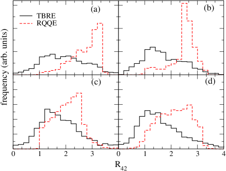
Figure 1: Probability distribution of $R_{42}$ for TBRE (solid line) and RQQE (dashed line) for (a) ²⁴Mg; (b) ²⁸Si; (c) ²²O; (d) ⁴⁸Ca.

For a pairing system, one expects $R_{42}\sim 1$. Fig. 1 shows the distribution of $R_{42}$ over a thousand samples from the TBRE for several different many-fermion systems. All are peaked near 1 (pairing), but with broad distributions that include $R_{42}=2$ (vibration) and 3.33 (rotational).

Many-boson systems, in particular the IBM-1, have also been studied using the TBRE, also yielding a dominance of $J=0$ ground statesBF00 . In contrast to fermion systems, however, the distribution of $R_{42}$ is sharply peaked at 2 and 3.33. Bijker and Frank studied the ratio $\mathrm{B(E2:4_{1}^{+}\rightarrow 2_{1}^{+})/B(E2:2_{1}^{+}\rightarrow 0_{1}^{+})}$, which turns out for IBM-1 to be strongly correlated with $R_{42}$ and agrees with analytic algebraic limits; plots of such correlations we will call Bijker-Frank plots. This is interpreted as evidence for band structure in bosons systems with random interactions. The boson results have been successfully explained using a mean-field analysisBF01 .

There have been numerous papers “explaining” the fermion results; for reviews seeZAY04 ; ZV04 . Much of the focus has been on the predominance of $J=0$ ground states; few have considered band structure beyond $J=4$, save for a few exceptions JBD98 ; ZV04 . In Fig. 2 we give a correlation plot for for $R_{62}$ vs. $R_{42}$. Fig. 2(a) shows results using “realistic” interactions calculations in the $sd$ Wi84 and $pf$ gxpf1 shell; 2(b)-(d) are results for the TBRE in several different fermion systems. Somewhat surprisingly, we get a strong correlation that follows exactly the naive predictions for pairing, vibrational, and rotational collectivity. (Although we do not show it, this result does not appear in single-$j$ systems frequently used as testbeds for random interactions). This higher-order band structure is a challenge to any claim to understanding random interactions results for fermion systems. Although we do not show it, similar (and sharper) results occur in the IBM with random interactions.

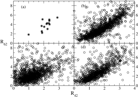
Figure 2: Correlation of $R_{62}$ vs. $R_{42}$ (a) ”realistic” calculations in $sd$ and $pf$ shells; TBRE in (b) ²⁴Mg; (c) ⁴⁴Ti; (d) ⁴⁸Ca.

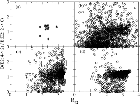
Figure 3: Bijker-Frank plots for fermion systems. (a) “Realistic” systems in the $sd$ and $pf$ shell. (b)-(d) for ²⁴Mg: (b) TBRE. (c) RQQE with standard quadrupole transition operator. (d) RQQE with ‘consistent’ transition operator.

Fig. 3 shows correlations of the ratio B(E2:$4\rightarrow 2$)/B(E2:$2\rightarrow 0$) vs. $R_{42}$ (Bijker-Frank plots), for “realistic” $sd$ and $pf$ shell calculations in Fig. 3(a), and for the TBRE in ²⁴Mg in Fig. 3(b). (For the B(E2) transitions in TBRE, for lack of other constraints we assume harmonic-oscillator radial wavefunctions.) While IBM-1 Bijker-Frank plots show sharp correlations, the fermion TBRE does not show very strong correlations. (Another approach to collectivity in fermion systems with random interactions is the Alaga ratioZV04 ).

Fig. 4 shows correlations between B(E2:$6\rightarrow 4$)/B(E2:$2\rightarrow 0$) and B(E2:$4\rightarrow 2$)/B(E2:$2\rightarrow 0$), which has not been previously studied. Again, Fig. 4(a) shows realistic results, while Fig. 4(b) is for the TBRE. The correlations are sharper than for the Bijker-Frank plot. Not shown are results for IBM-1, which has still sharper correlations.

To summarize: fermion systems with TBRE interactions show some signatures of collectivity, but much more weakly than boson systems. Why is not understood. This motivates the next section.

III The random quadrupole-quadrupole ensemble (RQQE)

One way to probe the difference between random interactions in boson and fermion systems is to search for a random ensemble that yield stronger collective structure in fermion systems. One proposal is the displaced TBRE, or DTBRE, where the two-body matrix elements are given a constant displacement. While an appealing suggestion, we have found that the DTBRE displays collective behavior only for a handful of even-even systems. Even worse, as discussed below, the resulting ensemble is not very “random.”

Therefore, inspired by the “consistent-Q” formulation in the interacting boson modelBF00 , we propose the following. Consider the general one-body operator of angular momentum rank 2:

$$\tilde{Q}_{m}=\sum_{ij}q_{ij}\left[\hat{a}_{i}^{\dagger}\times\hat{a}_{j}\right]_{2m}.$$ (4)

If $q_{ij}=\langle i||r^{2}Y_{2}||j\rangle$, then $\tilde{Q}$ is the standard quadrupole operator. But instead we choose the $q_{ij}$ randomly. We then define the random quadrupole-quadrupole ensemble to be interactions

$$\hat{H}=-\lambda\tilde{Q}\cdot\tilde{Q}.$$ (5)

The antisymmeterized matrix elements are $V_{ijlk}=q_{ik}q_{jl}-q_{il}q_{jk}$ (here and above we have left out details of the angular momentum coupling which are straightforward, if tedious, to include). There is also a one-body single-particle energy induced by normal ordering of the operators.

Any member interaction of the RQQE has fewer random parameters than the TBRE. For example, in the $sd$ shell, the TBRE has 63 independent, randomly generated two-body matrix elements, while the RQQE, if one assumes time-reversal symmetry (that is, $q_{ab}=(-1)^{j_{a}-j_{b}}q_{ba}$), has only 5 independent parameters; for the $pf$ shell, the TBRE has 195 independent matrix elements and the RQQE has 9.

The RQQE has $J=0$ ground states $>99\%$ for all even-even nuclides we tried. In Figs. 1-4 we show other results for the RQQE alongside those for the TBRE. To summarize them:

$\bullet$ In Fig.  1 we see $R_{42}$ for the RQQE peaks between 2 and 3.3, that is, somewhere between vibrational and rotational.

$\bullet$ Although not shown, the correlation of $R_{62}$ vs. $R_{42}$ for the RQQE is similar to that of the TBRE in Fig. 2.

$\bullet$ In Fig. 3(c)-(d), the Bijker-Frank plot shows the correlation between ratios of B(E2)s and $R_{42}$. Unlike in the TBRE, the RQQE shows much stronger correlation. Fig. 3(c) uses the “standard” quadrupole transition operator, assuming harmonic oscillator single-particle states; Fig. 3(d) uses a “consistent” quadrupole transition operator, the same $\tilde{Q}$ used in the Hamiltonian. Both results are similar, although the consistent-quadrupole results are sharper.

$\bullet$ In Fig. 4(c)-(d) we show correlations in B(E2)s in the yrast band 6-4-2-0. The correlations are much sharper than for the TBRE, and sharpest for the consistent-quadrupole calculation.

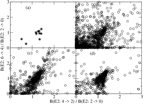
Figure 4: Correlation of B(E2) ratios B(E2: 6 $\rightarrow$ 4) / B (E2: 2 $\rightarrow$ 0) versus B(E2: 6 $\rightarrow$ 4)/B(E2: 2 $\rightarrow$ 0) for (a) “Realistic” systems in the $sd$ and $pf$ shell. (b)-(d) for ²⁴Mg: (b) TBRE. (c) RQQE with standard quadrupole transition operator. (d) RQQE with ‘consistent’ transition operator.

IV Test for randomness

Although the RQQE shows stronger spectral signatures for band structure in fermion systems than the TBRE, because the former has many fewer random parameters than the latter, we are concerned if the RQQE results are truly ‘random.’ We propose the following as a necessary, if not sufficient, test of randomness.

For any given many-fermion system, let $N_{0}$ be the dimension of the $J=0$ subspace. Therefore, any $J=0$ wavefunction can be represented as a vector of unit length in an $N_{0}$-dimensional space. If we choose the vectors randomly, then they will uniformly cover a unit sphere, and it is straightforward to show that the angle $\theta$ between any two vectors will have a probability $\propto\sin^{N_{0}-2}\theta$.

We compared ground state vectors for $J=0$ ground state. (We ignored interactions that did not have have $J=0$ ground states. ) We took the dot product between two randomly chosen ground state vectors, computed the angle between them, and binned the results, shown in Fig. 5 for ⁴⁸Ca. The expected $\sin^{(N_{0}-2)}\theta$ is shown for comparison.

Fig. 5(a) shows the distribution for the fermion TBRE. It follows exactly the expected $\sin^{(N_{0}-2)}\theta$ form.

Fig. 5(b) shows the distribution for RQQE. It is closer to the expected $\sin^{(N_{0}-2)}\theta$ than the DTBRE in (c) and (d) but is not completely random. The distortion may be due to the low number of independent random parameters.

Fig. 5 (c) and (d) shows the distribution for the displaced TBRE (DTBRE) for displacements $c\approx 1,3$, respectively. (Following the original paper, the width of the displaced Gaussian is 0.6.) Note as displacement $c$ gets larger, the distribution moves further from $\sin^{N_{0}-2}\theta$ and becomes more peaked towards $\theta=0$. These ground state wavefunctions are not randomly distributed; rather they are clustered about the limit wavefunction for $c\rightarrow\infty$.

This is strong evidence that TBRE wavefunctions are randomly and uniformly distributed; it is also evidence that the DTBRE wavefunctions are not uniformly distributed. The results from RQQE are inconclusive; they are not uniformly distributed as the TBRE wavefunctions are, but they are “more random” than DTBRE.

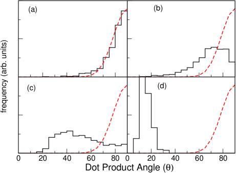
Figure 5: Distribution of angles between different $J=0$ ground state wavefunctions (for ⁴⁸Ca) for (a) TBRE; (b) RQQE; (c) DTBRE with displacement $c=1$; (d) DTBRE with displacement $c$ = 3. Dashed line is $\sin^{(N_{0}-2)}\theta$, where $N_{0}$ is the dimension of the $J=0$ subspace.

V Conclusions

We have revisited the question of signatures of collectivity in the spectra of random, two-body interactions in fermion systems. Some surprising, previously unknown correlations show up even in the two-body random ensemble (TBRE). We proposed a new “random” ensemble, the random quadrupole-quadrupole ensemble (RQQE), and found it had significantly sharper signatures of collectivity than the TBRE. While this does not solve the puzzle of collectivity, it does demonstrate that typical spectral signatures of collectivity do not rigorously require the standard Elliot quadrupole-quadrupole or SU(3) interaction.

Of course, collective behavior is not surprising if the “ensemble” is not very random, and we looked at the dot product between ground state wavefunctions: the RQQE deviates from the expected random distribution but much less so than the displaced TBRE or DTBRE.

The U.S. Department of Energy supported this investigation through grant DE-FG02-96ER40985.

References

- (1) A. Bohr and B. R. Mottelson, Nuclear Structure, Vol II (W. A. Benjamin, Inc., Boston, 1975).
- (2) I. Talmi, Simple Models of Complex Nuclei (Harwood Academic Publishers, Chur, Switzerland, 1993).
- (3) W. E. Ormand, REDSTICK shell model code (private communication).
- (4) C. W. Johnson, G. F. Bertsch, and D. J. Dean Phys. Rev. Lett. 80, 2749 (1998).
- (5) C. W. Johnson, Rev. Mex. Fiz. 45 suppl. 2 (1999) 25.
- (6) V. Velázquez and A. P. Zuker Phys. Rev. Lett. 88, 072502 (2002).
- (7) S. S. M. Wong and J. B. French, Nucl. Phys. A198, 188 (1972).
- (8) C. W. Johnson, G. F. Bertsch, D. J. Dean, and I. Talmi, Phys. Rev. C 61, 014311 (2000).
- (9) R. Bijker and A. Frank Phys. Rev. Lett. 84, 420 (2000).
- (10) R. Bijker and A. Frank, Phys. Rev. C 64, 061303 (2001).
- (11) V. Zelevinsky and A. Volya, Phys. Rep. 391, 311 (2004).
- (12) Y. M. Zhao, A. Arima, and N. Yoshinaga, Phys. Rep. 400, 1 (2004).
- (13) B. H. Wildenthal, Prog. Part. Nucl. Phys. 11, 5 (1984).
- (14) M. Honma, T. Otsuka, B.A. Borwn, and T. Mizusaki, Phys. Rev. C 69, 034335 (2004).