Thomas-Fermi theory for atomic nuclei revisited

Abstract

The recently developed semiclassical variational Wigner-Kirkwood (VWK) approach is applied to finite nuclei using external potentials and self-consistent mean fields derived from Skyrme interactions and from relativistic mean field theory. VWK consists of the Thomas-Fermi part plus a pure, perturbative $\hbar^{2}$ correction. In external potentials, VWK passes through the average of the quantal values of the accumulated level density and total energy as a function of the Fermi energy. However, there is a problem of overbinding when the energy per particle is displayed as a function of the particle number. The situation is analyzed comparing spherical and deformed harmonic oscillator potentials. In the self-consistent case, we show for Skyrme forces that VWK binding energies are very close to those obtained from extended Thomas-Fermi functionals of $\hbar^{4}$ order, pointing to the rapid convergence of the VWK theory. This satisfying result, however, does not cure the overbinding problem, i.e., the semiclassical energies show more binding than they should. This feature is more pronounced in the case of Skyrme forces than with the relativistic mean field approach. However, even in the latter case the shell correction energy for e.g. ²⁰⁸Pb turns out to be only $\sim-6$ MeV what is about a factor two or three off the generally accepted value. As an ad hoc remedy, increasing the kinetic energy by 2.5%, leads to shell correction energies well acceptable throughout the periodic table. The general importance of the present studies for other finite Fermi systems, self-bound or in external potentials, is pointed out.

I Introduction

One of the most important problems of finite fermion systems such as nuclei, atoms, helium- and metallic-clusters, quantum dots, etc., is the determination of the ground-state binding energy and the corresponding particle density distributions. In the nuclear case, to overcome the problems encountered when starting from realistic bare nucleon-nucleon forces, approximate and phenomenological schemes have widely been employed. This is the case of the very successful density dependent Hartree-Fock method with Skyrme Sky or Gogny Gog forces in the non-relativistic framework and of the relativistic mean field theory (non-linear $\sigma-\omega$ model) SW in the relativistic formulation.

To investigate how properties of global character vary with the number of nucleons $A$, which is the subject of the present work, semiclassical or statistical techniques are very useful. The best known example is the nuclear mass formula, based on the liquid drop or droplet model Myers . The success of the mass formula in describing binding energies lies in the fact that the quantal effects, i.e. shell corrections, are small as compared with the part of the energy which smoothly varies with $A$. The perturbative treatment of the shell correction energy in finite Fermi systems was elaborated by Strutinsky in the case of nuclei Strut . It was proposed to divide the total quantal ground state energy in two parts:

$$E=\tilde{E}+\delta E.$$ (1)

The by far largest part, $\tilde{E}$, varies smoothly with the number of fermions and is to be associated with the liquid drop energy. It can be calculated from e.g. the Hartree-Fock (HF) approach using the Strutinsky smoothing method Strut , which is a well defined mathematical procedure to erase the quantal oscillations in a finite Fermi system. However, this method may in general be more difficult to handle than the solution of the full quantal problem if realistic potentials are used. Thus, the search of alternative methods is an interesting and still partly open problem, as we will see. Semiclassical methods of the Thomas-Fermi (TF) type, which evaluate the smooth part of the energy, have widely been used in atomic, nuclear and metallic clusters physics. These TF methods, like the liquid droplet or Strutinsky calculations, smooth the quantal shell effects and estimate the average part of the HF energy BP ; Swia .

The semiclassical methods of the TF type are usually based on the Wigner-Kirkwood (WK) expansion of the density matrix WK . In this approach, the single-particle density $\rho$ and the kinetic energy density $\tau$ are expressed by means of functionals of the one-body single-particle mean field potential $V$. The $\hbar^{2}$ or $\hbar^{4}$ corrections to the lowest-order TF term contain gradients of $V$ of second or fourth order that arise from the non-conmutativity between the momentum $\hat{{\bf p}}$ and position $\hat{{\bf R}}$ operators. The $\hbar$ corrections to the pure TF particle or kinetic energy densities are known to diverge at the classical turning point. They are to be considered rather as distributions than as functions RS ; KCM , in the sense that only integrated quantities have a real physical meaning. It has been shown that, in the case of a harmonic oscillator potential well, the WK theory including up to $\hbar^{4}$ corrections is equivalent to the Strutinsky average BP .

An important property of the WK expansion of the energy in powers of $\hbar$ concerns its variational content. For a set of non-interacting fermions submitted to an external potential, as for instance harmonic oscillator or Woods-Saxon wells, the variational solution for the particle density which minimizes the semiclassical WK energy at each order of the $\hbar$ expansion, is just the WK expansion of the particle density $\rho$ at the same order in $\hbar$ SV ; CVDSE . The method for solving this variational problem SV ; CVDSE , which sorts out properly the different powers of $\hbar$ at each step of the minimization, was called variational Wigner-Kirkwood (VWK) theory. This VWK method has been applied to describe half infinite nuclear matter in the self consistent case using Skyrme forces CVDSE and the relativistic mean field approximation ECV . The formal VWK approach, up to $\hbar^{4}$ order, was developed in CVDSE .

Another related approach widely used for dealing with the semiclassical approximation of the self consistent HF problem, is based on the so-called density functional theory (DFT). The theoretical justification of DFT is formally provided by the Hohenberg and Kohn theorem HK . In the nuclear context it states that the energy of a set of interacting nucleons is a unique functional of the local density alone, that is

$$E=\int d\vec{r}\varepsilon\big{[}\rho(\vec{r})\big{]}.$$ (2)

which reaches its minimal value when calculated with the exact ground-state density. The ground-state density $\rho(\vec{r})$ is determined by a variational approach of Eq.(2) with the constraint of a fixed number of particles:

$$\frac{\delta}{\delta\rho}\int d\vec{r}\{\varepsilon\big{[}\rho(\vec{r})\big{]}-\mu\rho(\vec{r})\}=0.$$ (3)

In spite of the appeal of Eqs. (2) and (3), in general the exact energy functional is unknown and approximate techniques have to be worked out. The most popular and successful semiclassical approach based on DFT and developed together with the use of the Skyrme forces is the extended Thomas-Fermi (ETF) method. There the WK $\hbar$ expansion of the density is inverted to recast the kinetic energy density as a functional $\tau[\rho]$ of the local density and its derivatives GV ; BGH . If the potential part of the energy density is also a known functional of $\rho(\vec{r})$, as it happens for the Skyrme forces, the approximate energy density functional can be minimized to obtain an Euler-Lagrange equation like in Eq.(3). The solution of this equation will provide the ground-state particle density and energy. The quantum shell oscillations are absent in the ETF model, which yields average densities and energies with good accuracy BGH ; CPVGB ; PS ; Li ; BB ; CVBS ; CV .

Using the VWK method, we have studied in Refs.SV ; CVDSE the surface energy of a half infinite Fermi gas embedded in an external Woods-Saxon potential well. When $\hbar^{2}$ corrections are taken into account, the VWK surface energy reproduces the quantal values within 1% and the agreement is almost perfect when $\hbar^{4}$ corrections are considered. This result indicates that quantal Friedel oscillations have a negligible influence on the nuclear surface energy. We also have solved this problem using ETF (that in the case of the external potential reduces to the use of the ETF kinetic energy density). However, in this case we find discrepancies between ETF and quantal surface energies of 10% and 7% considering $\hbar^{2}$ and $\hbar^{4}$ corrections, respectively. This is an indication that ETF results are less well converged than the VWK ones. As it also will be discussed later on, this is mainly due to the fact that VWK properly sorts out the different orders in $\hbar$ which is not the case in ETF.

In Ref.CVDSE we have analyzed the surface energy in self consistent problems using the TF, VWK, and ETF (up to $\hbar^{2}$ order) semiclassical approaches in comparison with the quantal (HF) results. In this study we considered several Skyrme forces that cover a wide range of effective mass values and incompressibility moduli in bulk matter at saturation. In general the VWK2 surface energies are closer to the quantal values than the TF ones. (We call VWK2 the VWK theory developed up to order $\hbar^{2}$, similarly VWK4 for the theory up to order $\hbar^{4}$, and analogously for the ETF theory.) The ETF2 surface energies are systematically smaller than the corresponding quantal values, and their absolute error is always larger than in the VWK2 case. An analysis of VWK and ETF calculations of half infinite nuclear matter in relativistic mean field theory yields the same kind of conclusions and the quality of the VWK2 results is seen to be systematically better than in ETF2 ECV . However, if one compares the situation in the case of self consistent mean fields with respect to the case of the external Woods-Saxon potential well, the agreement between the semiclassical and quantal calculations of the surface energy worsens in the self consistent case, pointing to the fact that in the self consistent problems the semiclassical $\hbar$-expansions are more involved than in the case of an external potential. This aspect will be treated with more detail along this paper.

Summarizing, from the previous discussion it is clear that the VWK and ETF methods exhibit small but significant differences SV ; CVDSE ; ECV . The reason lies in the fact, as already mentioned, that ETF does not properly sort out the different powers in $\hbar$ and that it partially sums terms to all orders in $\hbar$. On the other hand, our previous findings in the study of the surface energy in the self consistent case SV ; CVDSE ; ECV indicate that the splitting of the quantal binding energies into their smooth and fluctuating parts is not so well under control (both in ETF and in VWK) as in the case of an external potential.

The main purpose of this paper is to develop and apply the VWK theory to finite nuclei in the self consistent case using both non-relativistic Skyrme forces and relativistic mean field (RMF) interactions SW . In the next section we present the basics of the VWK method in the non-relativistic case with an alternative derivation to the one used in Refs. SV ; CVDSE to explicitly show the differences between the VWK and ETF methods. In section III we first discuss within WK the external potential case to set the stage for the study of finite nuclei with self consistent mean fields later. We show that for strongly triaxially deformed mean field potentials with absence of any degeneracies, the semiclassical energies are extremely close to the quantal ones. Approaching sphericity in a homothetic way the shell structure becomes more and more apparent. Spherical open shell nuclei are slightly less bound quantally than semiclassically. This gives rise for the binding energy per particle as a function of particle number to the typical quantal arch structure between magic numbers whereas the semiclassical curve is, of course, monotonous. Section IV is devoted to the self consistent problem in finite nuclei. First, in section IV.A, we will show that using Skyrme forces, the VWK2 and ETF4 approaches practically give the same energy along the periodic table and that this fact is independent of the Skyrme interaction chosen. This a priori satisfying feature reveals, however, that the semiclassical approaches VWK2 and ETF4 overbind in excess, since even for the doubly magic nucleus ⁴⁰Ca the Hartree-Fock results gives less binding than the semiclassical ones. This is shown and discussed in section IV.B, where also an ad hoc remedy to this problem is proposed. Several technical aspects are discussed in Appendices 1 and 2.

II The variational Wigner-Kirkwood theory

The VWK theory has formally been introduced in Refs. SV ; CVDSE ; ECV . Here we present, for a non-relativistic Skyrme force, a shortcut derivation in order to show explicitly the similarities and differences with the ETF method. For the sake of simplicity we consider symmetric and uncharged nuclei for the moment and, in this section, a Skyrme force with an effective mass equal the physical one. In this case the total energy of a nucleus in the ETF approach up to order $\hbar^{2}$ (ETF2) is written as BGH ; CPVGB :

$$E=\int d\vec{r}\{\frac{\hbar^{2}}{2m}\big{[}\frac{3}{5}\big{(}\frac{3\pi^{2}}{2}\big{)}^{2/3}\rho^{5/3}+\frac{1}{36}\frac{(\nabla\rho)^{2}}{\rho}+\frac{1}{3}\Delta\rho\big{]}+a_{0}\rho^{2}+a_{3}\rho^{2+\alpha}+a_{12}\,(\nabla\rho)^{2}\},$$ (4)

where $a_{0}=3t_{0}/8$, $a_{12}=(9t_{1}-5t_{2}-4t_{2}x_{2})/64$, $a_{3}=t_{3}/16$, and $\alpha$ are the parameters that characterize the Skyrme interaction. The terms inside square brackets correspond to the ETF kinetic energy density $\tau_{ETF}$ up to $\hbar^{2}$ order. The $\rho^{5/3}$ term is the well-known pure TF contribution, which is of order $\hbar^{0}$ in the expansion of the kinetic energy density in $\hbar$ powers. The two remaining terms are of $\hbar^{2}$ order, and the first one is the so-called Weizsäcker term. Clearly, $\tau_{ETF}$ is a functional of the local density where the gradient terms are of second order in $\hbar$.

Starting from Eq.(4) the Euler-Lagrange equation for the local density constrained to give $A$ nucleons reads:

$$\frac{\hbar^{2}}{2m}\bigg{[}\bigg{(}\frac{3\pi^{2}}{2}\bigg{)}^{2/3}\rho^{2/3}+\frac{1}{36}\frac{(\nabla\rho)^{2}}{\rho^{2}}-\frac{1}{18}\frac{\Delta\rho}{\rho}\bigg{]}+2a_{0}\rho+(2+\alpha)a_{3}\rho^{1+\alpha}-2a_{12}\,\Delta\rho=\mu,$$ (5)

where the chemical potential $\mu$ is the Lagrange multiplier that ensures the right normalization of the local density $\rho$. In the ETF method the variational equation (5) is solved numerically, for instance using the imaginary-time step method CPVGB . However, the ETF approximation has some consistency problems with respect to the correct sorting out of powers in $\hbar$ CVDSE . The reason is that the solution of Eq. (5) contains $\hbar$ at all orders due to the fact that the Weizsäcker term in Eq.(4) is of order $\hbar^{2}$. Actually Eq.(5) has a similar structure as a Schrödinger equation for $\rho$ and thus the density contains $\hbar$ as an essential singularity SV .

In order to properly sort out the different powers in $\hbar$ (to second order in the present example) one should split the local density and chemical potential entering in Eq.(5) into their $\hbar^{0}$ and $\hbar^{2}$ parts:

$$\rho=\rho_{0}+\hbar^{2}{\rho_{2}}$$ (6)

and

$$\mu=\mu_{0}+\hbar^{2}\mu_{2}.$$ (7)

Using (6) and (7), the Euler-Lagrange equation (5) can be sorted into $\hbar^{0}$ and $\hbar^{2}$ terms. One key point in the VWK theory is that the minimization is performed for each order in the expansion parameter $\hbar^{2}$ separately since, in principle, $\hbar$ can be considered as an arbitrary parameter (see Refs. SV ; CVDSE ; ECV for a more detailed discussion of this point). Thus from the Euler-Lagrange equation (5) one obtains

$$\frac{\hbar^{2}}{2m}\big{(}\frac{3\pi^{2}}{2}\big{)}^{2/3}\rho_{0}^{2/3}+2a_{0}\rho_{0}+(2+\alpha)a_{3}\rho_{0}^{1+\alpha}-2a_{12}\,\Delta\rho_{0}-\mu_{0}=0$$ (8)

at TF ($\hbar^{0}$) order, and

$$\frac{\hbar^{2}}{2m}\big{[}\frac{2}{3}\big{(}\frac{3\pi^{2}}{2}\big{)}^{2/3}\rho_{0}^{-1/3}{\rho_{2}}+\frac{1}{36}\frac{(\nabla\rho_{0})^{2}}{\rho_{0}^{2}}-\frac{1}{18}\frac{\Delta\rho_{0}}{\rho_{0}}\big{]}$$ (9)

$$+ 2a_{0}{\rho_{2}}+(2+\alpha)(1+\alpha)a_{3}\rho_{0}^{\alpha}{\rho_{2}}-2a_{12}\,\Delta{\rho_{2}}-\mu_{2}=0$$

for the linearized second order correction. Another important point in the VWK theory is that the TF local density $\rho_{0}$, i.e. the variational solution of Eq.(8), fulfills the normalization condition:

$$\int d\vec{r}\rho_{0}=A$$ (10)

and due to the fact that

$$\int d\vec{r}\big{(}\rho_{0}+\hbar^{2}{\rho_{2}}\big{)}=A,$$ (11)

we immediately see that the integral over the second-order density vanishes. This condition can be assured in adjusting $\mu_{2}$.

Now, splitting the total energy $E$ into its $\hbar^{0}$ and $\hbar^{2}$ contributions and using Eqs. (8), (10) and (11), one finds that in the VWK approach the energy of a finite nucleus including corrections of order $\hbar^{2}$ can be written as:

$$E=\int d\vec{r}\{\frac{\hbar^{2}}{2m}\big{[}\frac{3}{5}\big{(}\frac{3\pi^{2}}{2}\big{)}^{2/3}\rho_{0}^{5/3}+\frac{1}{36}\frac{(\nabla\rho_{0})^{2}}{\rho_{0}}+\frac{1}{3}\Delta\rho_{0}\big{]}+a_{0}\rho_{0}^{2}+a_{3}\rho_{0}^{2+\alpha}+a_{12}\,(\nabla\rho_{0})^{2}\}.$$ (12)

Thus we arrive at the important result that the total energy up to order $\hbar^{2}$ is computed using only the lowest-order solution (TF) of the Euler-Lagrange equation. In practice this amounts to take the expression of the total energy as formally given by ETF2 but to compute it with the TF density solution. Consequently, the VWK procedure is consistent with the spirit of perturbation theory, since to calculate the energy at order $\hbar^{2}$ only requires knowledge of the solution of $\rho$ to the previous ($\hbar^{0}$) order SV ; CVDSE ; ECV . The integral in Eq. (12) is defined between $r=0$ and the classical turning point $r_{t}$ where the TF density $\rho_{0}$ vanishes. The analysis of Eq. (12) near $r_{t}$ shows that $\rho_{0}$ behaves as $(r_{t}-r)^{2}$ and, as a consequence, the integrand of (12) is always finite in the whole domain of definition.

Of course the procedure can be continued to obtain the fourth order correction, see Ref.CVDSE where this has been worked out in a slightly different way. The fourth order is, however, much more complicated, and necessitates for instance the knowledge of ${\rho_{2}}$ which may not easily be accessible CVDSE . We remark that ${\rho_{2}}$ is not needed in VWK2 for the calculation of the energy. This is a consequence of the fact that the total energy is just the quantity that is minimized and then the use of the Euler-Lagrange equations allows to eliminate ${\rho_{2}}$ in the expansion of the energy. However, the evaluation of other quantities that are not minimized, e.g. kinetic energies or root mean square radii, etc., needs the explicit knowledge of ${\rho_{2}}$ when computed to $\hbar^{2}$ order.

It should be pointed out that in the general realistic case with effective mass different from the bare nucleon mass, inclusion of the spin-orbit potential, etc., the VWK2 method follows the same principle as in our schematic example. In practice one can take the corresponding ETF2 expression for the ground-state energy and replace $\rho(\vec{r})$ by its TF solution $\rho_{0}(\vec{r})$ which is the self consistent solution of the lowest-order variational TF equation. We refer the reader to Eqs. (A1)-(A5) of Ref. CEV for the detailed ETF2 expression of the energy in the case of realistic Skyrme forces.

The same VWK theory can be applied to finite range effective forces such as the Gogny interaction Gog although this case will not be treated explicitly in this paper. For this type of forces the semiclassical single-particle potential is not only position but also momentum dependent because of the finite range CVDSE . Then, in addition to the kinetic and spin-orbit $\hbar^{2}$ corrections to the energy, there is another $\hbar^{2}$ contribution coming from the exchange term. Due to the $k$-dependence of the single-particle potential, the effective mass also becomes momentum dependent, which introduces extra terms in the $\hbar^{2}$ energy not present in the case of local forces as the Skyrme ones. The reader can find in Ref. SV2000 a detailed discussion of the ETF approach in the case of a general finite-range effective force. In particular, the kinetic and exchange energy densities in this case are given by Eqs.(39) and (40) of that reference. On the other hand, we also will consider in this paper the VWK approach applied to the relativistic mean field theory for the description of nuclei. The relativistic model automatically contains the finite range, spin-orbit and density dependence of the nucleon-nucleon interaction. The basic relativistic VWK theory up to $\hbar^{2}$ order has been worked out in Ref. ECV and applied to the analysis of half infinite nuclear matter. In the case of finite nuclei the basic equations to be used for the VWK2 calculations are Eqs.(A7)-(A11) of Ref. CEV together with Eqs.(5.8)-(5.12) of Ref. CVBS computed with the solution of the relativistic TF equations.

III The external potential case

In order to get a deeper insight into the behavior of the semiclassical energies as compared with the quantal ones before the study of finite nuclei with the use of self consistent mean field potentials, we first analyze the simpler problem of a set of non-interacting fermions submitted to an external potential well. In this case the VWK solution up to $\hbar^{2}$ order is just the WK expansion of the local density SV ; CVDSE as pointed out in the Introduction. We will consider the model problems of harmonic oscillator and Woods-Saxon potentials. The discussion of the harmonic oscillator, apart of being of interest by itself as it is one of the most important model potentials in quantum mechanics, is relevant in different areas of physics beyond the context of atomic nuclei, such as confined electron systems or trapped ultracold fermion gases. A separate study for the harmonic oscillator potential including deformation degrees of freedom and the problem of a cavity with sharp boundaries, where the WK expansion cannot be applied, will be presented in a forthcoming publication Leboeuf06 .

One important quantity is the number of states (accumulated level density) up to an energy $\varepsilon$, which is defined as RS

$$N(\varepsilon)=\int^{\varepsilon}_{0}g(\varepsilon^{\prime})d\varepsilon^{\prime}.$$ (13)

The level density $g(\varepsilon)$ is given by

$$g(\varepsilon) = {\rm Tr}\/[\delta(\varepsilon-{\hat{H}})]=\frac{\partial}{\partial\varepsilon}{\cal{L}}^{-1}_{\beta\to\varepsilon}\bigg{[}\frac{2}{(2\pi\hbar)^{3}}\int\int\frac{C^{\beta}(\vec{r},\vec{p})}{\beta}d\vec{r}d\vec{p}\bigg{]}$$ (14)

$$= \frac{2}{(2\pi\hbar)^{3}}\int\int\frac{\partial f_{\varepsilon}(\vec{r},\vec{p})}{\partial\varepsilon}d\vec{r}d\vec{p}$$

where ${\cal{L}}^{-1}_{\beta\to\varepsilon}$ is the inverse Laplace transform and the factor 2 takes into account spin degeneracy. We use the notation $C^{\beta}(\vec{r},\vec{p})$ for the Wigner transform of the single-particle propagator $\hat{C}^{\beta}=\exp{(-\beta\hat{H})}$, and $f_{\varepsilon}(\vec{r},\vec{p})$ is the corresponding Wigner function whose semiclassical expansion up to order $\hbar^{2}$ reads RS

$$f_{\varepsilon}(\vec{r},\vec{p}) = \Theta(\varepsilon-H_{\rm w})-\frac{\hbar^{2}}{8m}\Delta V\delta^{\prime}(\varepsilon-H_{\rm w})$$ (15)

$$+ \frac{\hbar^{2}}{24m}\big{[}(\nabla V)^{2}+\frac{1}{m}(\vec{p}\cdot\nabla)^{2}V\big{]}\delta^{\prime\prime}(\varepsilon-H_{\rm w}),$$

where $H_{\rm w}$ is the classical mean field Hamiltonian (Wigner transform of ${\hat{H}}$).

Inserting Eq.(14) into (13) one obtains the accumulated level density from the Wigner function as

$$N(\varepsilon)=\frac{2}{(2\pi\hbar)^{3}}\int\int f_{\varepsilon}(\vec{r},\vec{p})d\vec{r}d\vec{p}.$$ (16)

In the same way the energy of a set of fermions in a potential well filled up to the Fermi energy $\varepsilon$ can be expressed as

$$E(\varepsilon)=\int^{\varepsilon}_{0}\varepsilon^{\prime}g(\varepsilon^{\prime})d\varepsilon^{\prime}=\frac{2}{(2\pi\hbar)^{3}}\int\int f_{\varepsilon}(\vec{r},\vec{p})H_{\rm w}d\vec{r}d\vec{p}.$$ (17)

To simplify the calculation of $N(\varepsilon)$ and $E(\varepsilon)$, it is helpful to realize that $H_{\rm w}$ is the natural variable for $f_{\varepsilon}(\vec{r},\vec{p})$. In particular, the classical spherical harmonic oscillator (HO) Hamiltonian $H_{\rm w}=p^{2}/2m+m\omega^{2}r^{2}/2=P^{2}+Q^{2}$ can be seen as the square of a radial component $\sqrt{P^{2}+Q^{2}}$ in polar coordinates, with a polar angle $\theta=\arctan(P/Q)$. In a similar way, for a more general potential with spherical symmetry, radial and polar angle coordinates can be defined in phase space by

$$\sqrt{\tilde{H}_{\rm w}}=\sqrt{H_{\rm w}-V(0)},$$ (18)

where $V(0)$ is the bottom of the potential, and

$$\frac{p^{2}}{2m}=\tilde{H}_{\rm w}\sin^{2}\theta,\qquad V(\vec{r})-V(0)=\tilde{H}_{\rm w}\cos^{2}\theta.$$ (19)

This allows switching from the variables $(r,p)$ to the new ones $(H_{\rm w},\theta)$ in the integrals over phase space. An advantage of this procedure is that one automatically circumvents the divergency problems usually encountered at the classical turning point when the $\hbar^{2}$ corrections are taken into account. We will use this method to obtain the results for the accumulated level density and energy as a function of $\varepsilon$ for an external Woods-Saxon potential that we will discuss later in this Section.

In the case of an external potential of HO type the integration of Eqs.(16) and (17) can be done analytically. The semiclassical expressions of the accumulated level density and energy read

$$N_{\rm WK}(\varepsilon)=\frac{1}{3}\bigg{(}\frac{\varepsilon}{\hbar\omega}\bigg{)}^{3}-\frac{1}{4}\frac{\varepsilon}{\hbar\omega}$$ (20)

and

$$E_{\rm WK}(\varepsilon)=\bigg{[}\frac{1}{4}\bigg{(}\frac{\varepsilon}{\hbar\omega}\bigg{)}^{4}-\frac{1}{8}\bigg{(}\frac{\varepsilon}{\hbar\omega}\bigg{)}^{2}-\frac{17}{960}\bigg{]}\hbar\omega,$$ (21)

respectively, where the contribution $-17\hbar\omega/960$ in the last equation comes from the $\hbar^{4}$ correction. Notice that in a HO potential there is no $\hbar^{4}$ correction in $N_{\rm WK}$ BP .

For the HO potential the quantal level density can also be obtained analytically BB ; BJ and reads:

$$g(\varepsilon)=\frac{1}{\hbar\omega}\bigg{[}\bigg{(}\frac{\varepsilon}{\hbar\omega}\bigg{)}^{2}-\frac{1}{4}\bigg{]}\bigg{(}1+2\sum_{M=1}^{\infty}(-1)^{M}\cos\bigg{(}2\pi M\frac{\varepsilon}{\hbar\omega}\bigg{)}\bigg{)},$$ (22)

which is seen to split into a part that smoothly varies with $\varepsilon$ and a fluctuating part. The smooth part is equal to the semiclassical WK expansion of the level density up to $\hbar^{2}$ (as already mentioned, the contributions of higher order in $\hbar$ vanish for the HO potential). The fluctuating part corresponds to the shell correction and contains all the quantal effects not included in the WK expansion. The quantal expressions for the accumulated level density and energy can easily be calculated starting from Eq.(22):

$$N(\varepsilon) = N_{\rm WK}(\varepsilon)+2\sum_{M=1}^{\infty}(-1)^{M}\bigg{[}\frac{1}{4\pi^{2}M^{2}}\frac{\varepsilon}{\hbar\omega}\cos\bigg{(}2\pi M\frac{\varepsilon}{\hbar\omega}\bigg{)}$$ (23)

$$+ \bigg{(}\frac{1}{2\pi M}\bigg{(}\frac{\varepsilon}{\hbar\omega}\bigg{)}^{2}-\frac{1}{4\pi^{3}M^{3}}-\frac{1}{8\pi M}\bigg{)}\sin\bigg{(}2\pi M\frac{\varepsilon}{\hbar\omega}\bigg{)}\bigg{]}$$

and

$$E(\varepsilon) = E_{\rm WK}(\varepsilon)+2\sum_{M=1}^{\infty}(-1)^{M}\bigg{[}\bigg{(}\frac{3}{4\pi^{2}M^{2}}\bigg{(}\frac{\varepsilon}{\hbar\omega}\bigg{)}^{2}-\frac{3}{8\pi^{4}M^{4}}-\frac{1}{16\pi^{2}M^{2}}\bigg{)}\cos\bigg{(}2\pi M\frac{\varepsilon}{\hbar\omega}\bigg{)}$$ (24)

$$+ \bigg{(}\frac{1}{2\pi M}\bigg{(}\frac{\varepsilon}{\hbar\omega}\bigg{)}^{3}-\frac{3}{4\pi^{3}M^{3}}\frac{\varepsilon}{\hbar\omega}-\frac{1}{8\pi M}\frac{\varepsilon}{\hbar\omega}\bigg{)}\sin\bigg{(}2\pi M\frac{\varepsilon}{\hbar\omega}\bigg{)}\bigg{]}\hbar\omega.$$

Therefore, in this simple model the separation of the total energy in a smooth (liquid drop like) part $\tilde{E}$ and a shell correction part $\delta E$, like in Eq.(1), is obtained analytically.

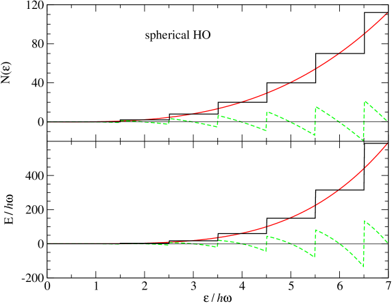
Figure 1: (Color online) Accumulated level density (upper panel) and total energy (lower panel) with degeneracy 2 for a fixed spherical harmonic oscillator potential as a function of the Fermi energy $\varepsilon$. Staircase, solid, and dashed lines correspond to the quantal, semiclassical (WK with $\hbar^{4}$ corrections), and shell correction (quantal minus semiclassical) values, respectively.

The upper panel of Fig.1 displays the accumulated level density $N(\varepsilon)$ for a set of fermions in a fixed spherical HO potential calculated semiclassically and quantally, as a function of the Fermi energy $\varepsilon$ divided by $\hbar\omega$. The quantal result exhibits discontinuities at each major shell ($N=2$, 8, 20, 40, 70, and 112 in the figure) and is represented by a staircase function formed by horizontal and vertical lines which fluctuate around the smooth value of $N(\varepsilon)$. The latter is provided by the WK value given by Eq.(20) and is represented by the solid curve of the upper panel of Fig.1. In the same panel we display the oscillatory part of $N(\varepsilon)$ (dashed curve), i.e., the quantal minus the semiclassical values, which contains the fluctuations due to the shell effects. One sees that the quantal part of the accumulated level density oscillates around zero.

The lower panel of Fig.1 displays the quantal and semiclassical WK values of the total energy $E(\varepsilon)/\hbar\omega$ for the spherical HO potential by the staircase and solid curves, respectively. In the same lower panel, the shell energy, i.e. the difference between the quantal and semiclassical values, is represented by the dashed line. Again it can be seen that the shell energy fluctuates around zero and that the semiclasical WK estimate of $E(\varepsilon)/\hbar\omega$ averages the quantal values. As it has been pointed out in the Introduction, the WK approach to $E(\varepsilon)$ including $\hbar^{4}$ corrections coincides with the Strutinsky average in the HO potential BP .

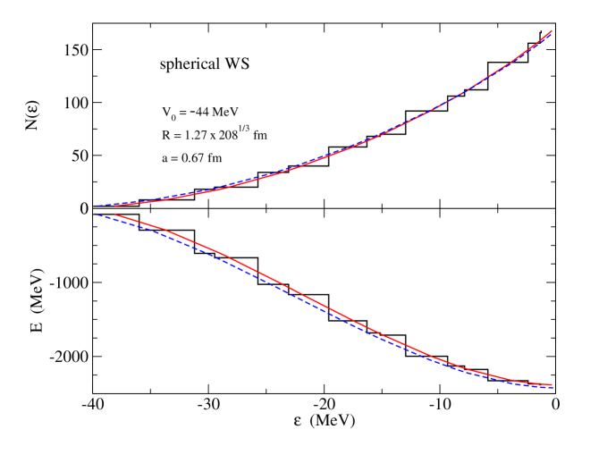
Figure 2: (Color online) Accumulated level density (upper panel) and total energy (lower panel) with degeneracy 2 for a fixed spherical Woods-Saxon potential as a function of the Fermi energy $\varepsilon$. Staircase lines correspond to the quantal values, while solid and dashed lines correspond to the semiclassical WK with $\hbar^{2}$ corrections and TF results, respectively.

We have performed the same kind of analysis for the more realistic potential well of Woods-Saxon (WS) type used in Ref. JBB : $V(r)=V_{0}/[1+\exp{(\frac{r-R}{a})}]$ with the values $V_{0}=-44$ MeV, $a=0.67$ fm and $R=1.27A^{1/3}$ fm. We have computed quantally and semiclassically (with pure TF and with WK up to $\hbar^{2}$ order) the accumulated level density and energy of neutrons (spin degeneracy is assumed) in the above WS potential with a size corresponding to a nucleus of $A=208$ nucleons. The calculated $N(\varepsilon)$ and $E(\varepsilon)$ are displayed as a function of the Fermi energy $\varepsilon$ in the upper and lower panels of Fig.2, respectively. Again the staircase and solid curves correspond to the quantal and WK results, respectively, whereas the dashed lines are now the pure TF values. As in the case of the HO potential, the WK estimate of the smooth parts of $N(\varepsilon)$ and $E(\varepsilon)$ passes well through the corresponding staircase functions and averages the quantal accumulated level density and energy.

For the WS potential the equivalence between the semiclassical WK expansion and the Strutinsky average cannot be established analytically. It has been checked numerically that both methods, with high accuracy, give the same value for the energy, at least in the case where the chemical potential is sufficiently negative RS ; CVDSE ; CPVGB ; JBB . However, the situation may be different when the Fermi energy is close to zero. In this case, the semiclassical WK and Strutinsky level densities start to deviate from one another when $\varepsilon$ approaches zero. The WK level density, which includes $\hbar^{2}$ corrections shows a ${\varepsilon}^{-1/2}$ divergency at $\varepsilon=0$ for a finite potential as the WS one, whereas the Strutinsky averaged level density only has a strongly pronounced, but finite, maximum S . In Refs. NWD ; VKLNSW it was concluded that the divergency of the WK level density for $\varepsilon\to 0$ is unphysical and preference should be given to the Strutinsky smoothed level density. However, we would like to recall that WK quantities have to be understood in the sense of distributions RS ; KCM . Therefore, a diverging WK level density should not be taken literally and only used under integrals. For example, in the upper and lower panels of Fig.2 one sees that the accumulated semiclassical level density $N(\varepsilon)$ and the total energy $E(\varepsilon)$ are well behaved and accurately average the corresponding quantal values even for $\varepsilon\to 0$. The TF accumulated level density and energy show similar tendencies to those exhibited by the WK results. However, the TF average of the quantal values is less good than the one obtained at the WK level. This fact demonstrates the importance of the $\hbar$-corrections in the Wigner function (15) to obtain the correct average of the quantal results.

Usually the various quantities like energy, kinetic energy, etc. for a system containing a fixed number of particles $N$ are not displayed as a function of the chemical potential $\mu$ [given by $N=N(\mu)$], but rather as functions of the particle number. For example, having the energy $E(\mu)$ and the accumulated level density $N(\mu)$ as functions of the chemical potential $\mu$ we can consider the inversion $\mu=\mu(N)$ and then obtain the energy as a function of the particle number $N$, i.e $E=E(N)$. The $N$ dependence can be studied for a fixed external potential. More realistically the potential well will change with the number of particles, as e.g. the HO potential with $\hbar\omega\simeq 41A^{-1/3}$ MeV or the WS potential of Ref. BB . Below we will consider both cases: the most simple case of a fixed potential well and the case where the potential changes with the particle number.

If the potential well has degenerate levels, the inversion $\mu=\mu(N)$ is not unambiguous in the quantal case, because the chemical potential is the same for various values of the particle number $N$. This is for example the case for the spherical HO. To get around this problem one can consider the spherical HO as the limit of a triaxially deformed HO in the limit of zero deformation. In the triaxial case each level has only spin-isospin degeneracy. However, for the purpose of our reasoning we here can disregard spin and isospin. Then in the infinitesimal triaxially deformed HO all levels can be occupied by only “one nucleon”. In the case of sphericity a major shell with HO principal quantum number $n$ has a degeneracy $D(n)$ and the functions $N(\mu)$ and $E(\mu)$ are sharp staircase functions, whereas for very small triaxial deformation the vertical jumps become slightly tilted and resolved in $D(n)$ minuscule staircases. In that case one then always has a definite number of particles for definite values of $\mu$ and perfectly can find $\mu=\mu(N)$ unambigously. Therefore also $E(N)$ is well defined. In the limit of zero deformation this leads to the uniform filling prescription of a degenerate shell at sphericity.

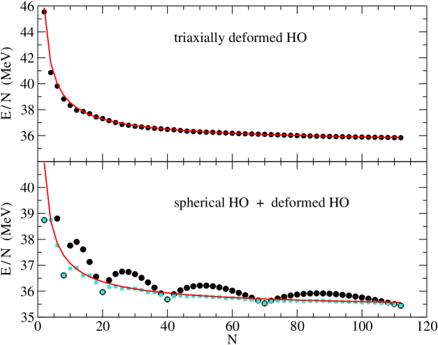
Figure 3: (Color online) Upper panel: quantal (dots) and WK (solid line) energy per particle in a strongly triaxially deformed size-dependent harmonic oscillator potential as a function of the number of particles. Lower panel: the same as in the upper panel but for a spherical size-dependent harmonic oscillator potential (notice that the semiclassical WK curves are different in the deformed and spherical cases). The squares depict the quantal energies per particle in the case that the deformation of the harmonic oscillator potential is optimized leading to maximal binding. Notice the close agreement with the semiclassical curve obtained for the spherical harmonic oscillator.

With these preliminaries in mind, we show in the upper and lower panels of Fig.3 the energy per particle as a function of the particle number for (i) a strongly deformed HO with frequencies

$$\omega_{x}=\sigma^{-1/3}\delta^{-1/2}\omega_{0},\qquad\omega_{y}=\sigma^{-1/3}\delta^{1/2}\omega_{0},\qquad\omega_{z}=\sigma^{2/3}\omega_{0},$$ (25)

taking the values $\omega_{x}=0.460\,\omega_{0}$, $\omega_{y}=1.111\,\omega_{0}$, and $\omega_{z}=1.954\,\omega_{0}$, and (ii) a spherical HO in the sense explained above. The HO depends as usual on particle number through $\hbar\omega_{0}=41A^{-1/3}$ MeV and deformation is such that volume is conserved ($\omega_{x}\omega_{y}\omega_{z}=\omega_{0}^{3}$). In the upper panel of Fig.3 we see that in the deformed potential BB the quantal values (dots) practically coincide with the WK values (solid line) and in any case WK perfectly averages the quantal values. On the other hand, in the spherical case there is a surprise in the sense that the WK-values do not pass, as a function of the particle number, through the average of the quantal values: there are much more values above the WK-line than below and also the deviations above the WK-line are stronger than below. This means that WK overbinds with respect to the true average except at magicity.

In the light of the fact that for the separate curves $E(\varepsilon)$ and $N(\varepsilon)$ (see Fig.1) the semiclassical values perfectly average the quantal ones also in the spherical case, the global overbinding of WK as a function of the particle number may appear puzzling. The effect is, however, known Leb . One can indeed show that an average over $\varepsilon$ (or $\mu$) of the fluctuating part in (24) yields zero, whereas when expressed as a function of $N$ the fluctuating part shows a non-vanishing average, i.e. $\langle\,\delta E(\mu)\,\rangle_{\mu}=0$ but $\langle\,\delta E(N)\,\rangle_{N}\neq 0$, where the brackets $\langle\,\dots\,\rangle_{\mu,N}$ indicate averages over $\mu$ or $N$, respectively. This feature can also be understood schematically from a different aspect in the following way. Suppose we consider a HO potential of fixed size with very small triaxial deformation, i.e. we consider the uniform filling prescription at sphericity. In a given shell the total quantal energy increases linearly with the number of nucleons in the shell. On the other hand, on average the total energy, according to Eqs. (20) and (21), increases at the TF level as $E_{tot}\propto N^{4/3}$. This situation is detailed in Table 1 for the $n$=4 shell of a spherical HO potential of fixed size, which contains the $1g$, $2d$ and $3s$ levels. There we display the quantal and semiclassical (TF and WK including $\hbar^{2}$ corrections) chemical potentials and energies obtained in filling uniformly the shell assuming spin degeneracy (the values are expressed in units of $\hbar\omega$). The semiclassical chemical potentials are obtained inverting Eq.(20) to find the corresponding value of $\mu$ which in turn is used in (21) to calculate the semiclassical energies. The quantal chemical potential in each spherical shell of the HO potential is given by $\mu/\hbar\omega=n+3/2$. The number of particles and energy in the $n$=4 shell are given by

$$N=\sum_{n=0}^{3}D(n)+2m=40+2m$$ (26)

and

$$\frac{E}{\hbar\omega}=\sum_{n=0}^{3}D(n)\bigg{(}n+\frac{3}{2}\bigg{)}+2m\bigg{(}4+\frac{3}{2}\bigg{)}=150+2m\bigg{(}4+\frac{3}{2}\bigg{)},$$ (27)

where $D(n)=(n+1)(n+2)$ is the degeneracy of a shell including spin and $m=1,2,3,\ldots$ is the number of pairs (spin up and spin down) added to fill up the $n$=4 shell. From Table 1 we see that the TF energies always overbind the quantal values and the same is true for the WK ones, except close to magicity where the $n$=4 shell is empty or completely full.

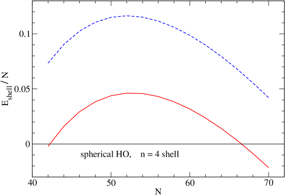
Figure 4: (Color online) WK2 (solid line) and TF (dashed line) shell energies, per particle, defined as the difference between the quantal and semiclassical energies (in $\hbar\omega$ units) filling the $n=4$ shell of a fixed spherical harmonic oscillator potential as a function of the number of the particles in the shell. The $\hbar^{4}$-corrections are indistinguishable from the solid VWK2-line.

The shell correction, i.e. the difference between quantal and semiclassical energies, is displayed in Fig.4 as a function of the number of particles in the shell. From this figure it is clear that the TF approach is far from averaging the quantal values and that in the WK case the average is much improved. If the $\hbar^{4}$ corrections are added, in this case of a fixed HO potential, the energy is shifted down by a constant amount of 17/960 (in $\hbar\omega$ units) according to Eq.(21), but it cannot be distinguished from the $\hbar^{2}$-corrected result on the scale of the figure. Therefore, the $\hbar^{4}$ corrections are very small as compared with the $\hbar^{2}$-ones demonstrating again the rapid convergence of the WK series. Thus, the situation for a fixed HO potential is similar to that found in the more general case of a size dependent HO potential as it can be seen comparing the lower panel of Fig.3 with Fig.4.

The lack of averaging in the energies found in the spherical potential is due to the large degeneracy of the HO shells. If each shell is broken into $D(n)$ small pieces, as in the case of strong triaxiality, they are bound to stay close to the average which varies, as already mentioned, as $\sim N^{4/3}$. In the case of sphericity this $N^{4/3}$ behaviour is, as demonstrated in Table 1, quantally replaced by straight line segments, each segment corresponding to a major shell. Two segments join at a magic number with a characteristic overbinding which is relatively small. In between two magic points the quantal straight line passes most of the time above the concave semiclassical curve. This scenario can further be clarified by the following investigation. The fact that for strong triaxiality quantal and semiclassical calculations almost agree can be understood because in that case there do not exist degeneracies (besides some special cases where the axis ratios are formed by rational numbers BJ ). Therefore, the quantal level density is also practically smooth, and it almost coincides with the semiclassical result.

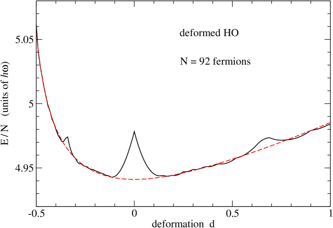
Figure 5: (Color online) Quantal (solid line) and WK (dashed line) values of the energy per particle of a set of 92 fermions submitted to a triaxilly deformed HO potential as a function of the deformation $d$ [Eqs.(25) and (28)]. Spin degeneracy is included.

In Fig.5 we show this, displaying the energy per particle as a function of triaxial deformation for a HO well. To have a single deformation parameter $d$ for the representation, in this figure we have chosen the frequencies of the deformed HO according to

$$\sigma=1+d\sqrt{3},\qquad\delta=1+|d|\sqrt{2}$$ (28)

in Eq. (25). We see that for a mid-shell configuration (spin degeneracy) of $N=92$ fermions, the semiclassical and quantal values practically agree, up to very small fluctuations, down to quite low deformations. The quantal energy suddenly raises when approaching sphericity. For real nuclei this means that binding energy is lost at sphericity. The only slight exception to this scenario is for deformation $\sim$ 0.6 where the frequency ratio is close to $\omega_{x}:\omega_{y}:\omega_{z}\sim 1:2:3$. We, therefore, see that in forcing open shell nuclei to be spherical one loses a lot of binding energy. As a matter of fact, this loss of binding energy starts immediately off magic numbers and increases towards mid shell fillings. This explains why the semiclassical curve mostly overbinds as a function of the shell filling. In the general case with mass number dependent potentials, these considerations are slightly more complicated but the reasoning which leads to the underbinding of quantal results for energies per particle keeping open shell nuclei spherical is essentially the same. This is one of the explanations of the fact that the shell corrections as a function of the particle number, do not oscillate around zero but show a finite average value. Above we already have mentioned that this can also be seen from the fact that as function of the particle number the fluctuating part in Eq.(24) does not average to zero Leb . Below we will find that the same situation prevails in the case of self consistent mean fields. We also would like to mention that similar features as those discussed above in connection with deformation and degeneracy of the single-particle levels have been found by Pomorski pomorski04 using the Strutinsky smearing method applied in energy space and in particle number space.

The above considerations only apply to spherical nuclei. In reality the force which holds semimagic nuclei, e.g. tin isotopes, spherical is the magicity of the protons which resists to deformation. For deformed nuclei the situation is different and needs separate investigation. In the lower panel of Fig. 3 we show what happens when the shape of the potential is free and the energy minimised for each particle number with respect to deformation. The absolute minimum of the quantal calculation is obtained allowing triaxial deformation in Eq.(25). Now the arches are strongly flattened and in between magic numbers the energies per particle lie practically on the semiclassical curve. Magic nuclei appear as exceptional points and a particle number average will be close to the semiclassical result. Notice again that we are now comparing absolute minima both in the semiclassical case (where they occur exclusively at sphericity) and in the quantal one (where they are deformed, besides around magicity). From this point of view, the close agreement between quantal and semiclassical results is very satisfying and it likely is a generic feature valid also for other types of mean field potentials. For real nuclei, deformed as well as spherical situations can happen. If both proton and neutron numbers correspond to open shell situations, nuclei are in their majority deformed, whereas if either the proton or neutron number is magic, nuclei usually are spherical, as it happens for instance for the chain of Sn isotopes. Because of the numerical complexity of the deformed case, we only will concentrate on spherical nuclei in the remainder of the paper. More detailed investigations of the deformed situation will be presented elsewhere Leboeuf06 .

The fact that the semiclassical results are not going through the average of the quantal results as a function of $A$ is somewhat annoying from the practical point of view, since we cannot judge whether the semiclassical results are converged to the right value or not. In the case of external potentials the answer to this question is easy to find: we take a fixed potential and look at the WK results as a function of the chemical potential $\mu$. We know that in this case the semiclassical results should pass through the average of the quantal ones (see e.g. Fig.2).

IV The self consistent potential case

IV.1 Finite nuclei

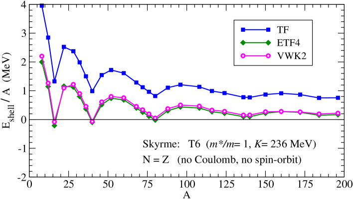
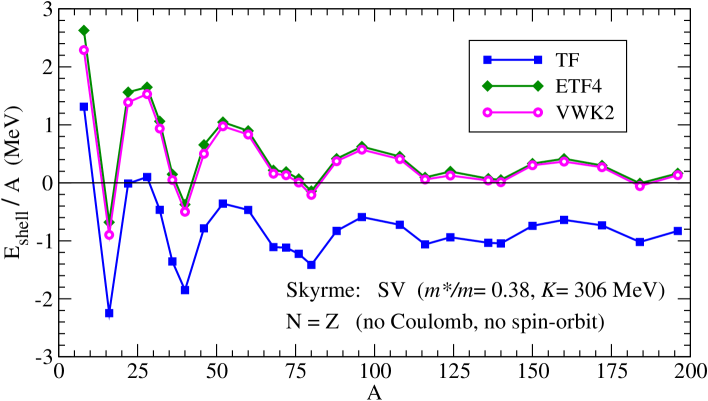
Figure 6: (Color online) Upper panel: Shell correction $E_{\rm shell}=E_{\rm HF}-E_{\rm semicl}$ in the TF, ETF4, and VWK2 approaches for symmetric uncharged nuclei without spin-orbit force as a function of the mass number $A$ calculated with the Skyrme force T6 T6 . Lower panel: the same for the Skyrme force SV Sk5 .

For spherical nuclei described self consistently through an effective interaction, the scenario for the energy per particle as a function of the mass number stays qualitatively the same as for the external potential case. Again, the typical arch structure with the values at magicity barely undershooting the semiclassical line (see lower panel of Fig.3) appears. In the upper panel of Fig.6 we present self consistent calculations of the shell energy per particle, which is defined as $E_{\rm shell}/A=(E_{\rm HF}-E_{\rm semicl})/A$, as a function of the mass number, for the TF, VWK2, and ETF4 semiclassical approaches using the T6 force T6 . This Skyrme interaction has an effective nucleon mass $m^{*}$ equal to the bare one $m$. In the calculations shown in Fig.6, the Coulomb repulsion among protons and the spin-orbit force have been switched off and only hypothetical spherical symmetric nuclei with $N=Z$ are considered. Later we will study realistic nuclei, but for the moment we want to avoid that these more subtle effects contaminate the comparison of the semiclassical results with the quantal ones.

The same type of calculation is presented in the lower panel of Fig.6, now performed using the very different Skyrme force SV Sk5 that has no density-dependent part ($t_{3}=0$) and for which the effective mass is $m^{*}/m$=0.38 in nuclear matter. In the case of the VWK2 calculation we encounter the same pattern as with the T6 force. However, the predictions of the TF calculation are at variance with the case of the T6 interaction: for T6 they overbind, whereas for SV they underbind. This change in the behaviour of the TF solution is largely due to the different values of the effective masses of the two forces, and we have documented this fact already in earlier publications CVDSE ; CVBML . Very satisfactorily, the deviation of the VWK2 results from the HF ones only depends very little on the particular properties of the effective interaction.

We have to remark the important feature that, as can be seen in Fig.6, the shell energies per particle calculated with the VWK2 and ETF4 approaches are very close. We have tested a whole series of Skyrme forces and did not find exceptions to this fact. As we will see below, the inclusion of Coulomb and spin-orbit forces does not change this rule essentially. Thus, with the VWK2 calculation one is able to obtain energies of an equivalent quality to the by far more complicated ETF4 approach which requires sophisticated techniques for the self consistent numerical solution of the variational equations.

Several additional comments should, however, still be made. Above we argued that ETF is inconsistent in sorting out the powers in $\hbar$ and that consequently it converges less well than VWK. We also gave arguments backed by explicit examples that VWK should converge faster than ETF and that the $\hbar^{4}$-contribution to VWK should practically be negligible. This was, however, for an external potential case. Perhaps the external potentials are particularly difficult cases for ETF (for instance one has to solve a non-linear differential equation even in the external potential case, whereas the WK expression can be used as is) and its convergence properties are better in the completely self consistent case. Thus, it could be that both the VWK2 (besides a small VWK4 correction as in the external potential case) and the ETF4 results are converged to the same and definite semiclassical value for nuclear binding energies. However, at this point this is a speculation. It may be that VWK2 and ETF4 coincide without both really having reached complete convergence to the actual semiclassical average. For instance, it cannot be excluded that VWK4 could, in the self consistent case, yield a contribution which is sensitively more important than in the external potential case. This remark should be kept in mind when we discuss the results more closely below.

The uncertainty of the situation also comes from the fact that, as discussed above, we do not have a precise criterion in the self consistent case what the semiclassical binding energies as a function of the particle number should be, besides that they should coincide with a Strutinsky self consistent calculation. The latter is, however, also slightly uncertain, because the plateau condition is difficult to satisfy BB ; Pom and up to date only a few self consistent Strutinsky calculations with Skyrme forces exist in the literature BQ ; BQ1 . However, in any case the general agreement of VWK2 with ETF4 is quite remarkable and adds more confidence to the semiclassical results, in spite of the fact that problems are not all resolved as we will further discuss below.

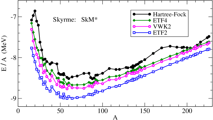
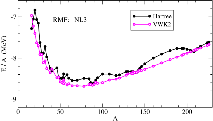
Figure 7: (Color online) Energy per nucleon of $\beta$-stable spherical nuclei along the periodic table calculated with the non-relativistic Skyrme force SkM^∗ (upper panel) and with relativistic mean field with parameter set NL3 (lower panel).

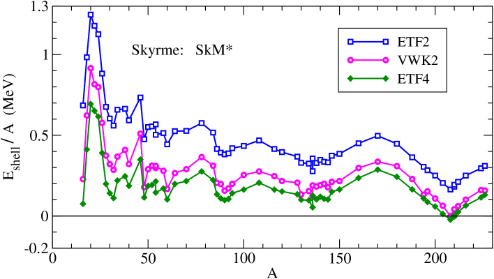
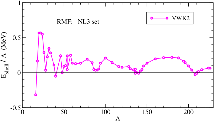
Figure 8: (Color online) Shell correction at VWK2 level of $\beta$-stable spherical nuclei as a function of the mass number $A$ calculated with the Skyrme force SkM^∗ (upper panel) and using relativistic mean field with parameter set NL3 (lower panel).

In order to give additional backing to what is just outlined with more studies, we now show on the upper panels of Figs.7 and 8 the energy and the shell correction per nucleon, respectively, in a realistic case for nuclei along the valley of stability calculated with the SkM^∗ interaction including the Coulomb and spin-orbit forces. Most of the $\beta$-stable nuclei displayed in Figs.7 and 8 were also used in Ref. Pom , and they are spherical according to the finite range droplet model (FRDM) FRDM1 . We have also considered some other additional nuclei which, according to the FRDM, are also $\beta$-stable FRDM1 and spherical except for a few of them FRDM2 . Also in this realistic case we can observe the very close agreement between the VWK2 and ETF4 methods. We also display the results of the ETF2 calculation and notice that it is much less converged. The VWK2 approach to the relativistic mean field theory has also been worked out ECV and we present the results for the same sample of nuclei along the valley of stability using the realistic, accurately calibrated parameter set NL3 NL3 on the lower panels of Figs.7 and 8. In the relativistic case the ETF4 corrections have not been elaborated and we do not have the corresponding results available. We have found the relativistic ETF2 results to be, as in the non-relativistic case, not so well converged as VWK2 and we do not show them.

In Fig.8 we quite clearly see a deficiency of the semiclassical energies, already present in the preceding figures: there is too much binding, even keeping in mind that the semiclassical binding energies for spherical nuclei have a natural tendency to be stronger than the average of the quantal values as discussed in section III. This drawback is particularly pronounced in the case of Skyrme forces (we checked this with multiple Skyrme interactions). Also in the relativistic case the semiclassical results give too much binding, in spite of the fact that the doubly magic nuclei are (slightly) more bound quantally than semiclassically, what is not the case for Skyrme forces, see Table 2. This situation clearly is unphysical. We will comment further on this in the next subsection. Let us point out that in our prescription the shell correction has been taken as $E_{\rm shell}=E_{\rm HF}-E_{\rm semicl}$, which in principle is different from the often employed prescription where one takes $E_{\rm shell}=\sum\varepsilon_{i}-\sum\varepsilon_{i}\tilde{n}_{i}$ as the difference of the sum of the quantal single-particle energies and the Strutinsky averaged sum. However, due to the Strutinsky energy theorem RS the predictions of both procedures should agree if the considered semiclassical approaches reproduce well the Strutinsky averaged value.

Concluding this subsection, we can say that the semiclassical limit of the energy per particle of finite nuclei based on Skyrme or relativistic mean field theories has been established on the VWK2 level. A quite intriguing coincidence between the VWK2 and ETF4 methods has been found. The significance of this fact is not entirely clear and will be discussed further in the next section. The ETF4 method exists since long whereas VWK2 is new. Apart from the discussed conceptual differences in the rigorous power counting in the $\hbar$ expansion, the VWK2 method, see Eq.(12), has the advantage that the convergence is faster and that the final formulas for the calculation $E/A$ are very simple (only the solution of the zeroth-order TF variational equation is needed!). The overbinding of TF and ETF calculations of nuclei has been recognized in many studies since years ago (see e.g. Refs. BGH ; CPVGB ; PS ; Li ; BB ; CVBS ; CV ; Kumar ; BCKT ), and it is also very much present in atomic physics calculations March . We have shown that the problem persists even in the more refined ETF4 and VWK2 appoaches, and we will turn to it in more detail now.

IV.2 The overbinding problem

In the last section we have seen that the scenario of the arch structure in the energy per particle remains in the self consistent case qualitatively the same as in the external potential case. However, we remarked a deficiency in the self consistent case which becomes apparent when having a close look at the realistic cases presented in Figs.7 and 8. In Table 2 we present the quantal and VWK2 energies for some magic nuclei calculated with the SkM^∗ force and with the NL3 parameter set of the relativistic theory. We see, that in particular Skyrme forces overbind semiclassically, as it is also seen in the upper panels of Figs.7 and 8. The fact that even doubly magic nuclei like ⁴⁰Ca are more bound semiclassically than quantally is clearly incorrect, even though we should be aware of the fact that we are dealing with small differences of large numbers. In any case, taking self consistent Strutinsky calculations as reference BQ ; BQ1 , ⁴⁰Ca and ²⁰⁸Pb are less bound, when averaged, than quantally. This failure of the semiclassical approach is disappointing with respect to the external potential case where, as a function of energy (or chemical potential), we are used to the fact that the VWK2 method gives extremely precise average quantities, like level densities, energies, etc., as has been demonstrated in the past with many examples RS ; BP ; SV ; CVDSE (see also Figs.1 and 2 of this paper).

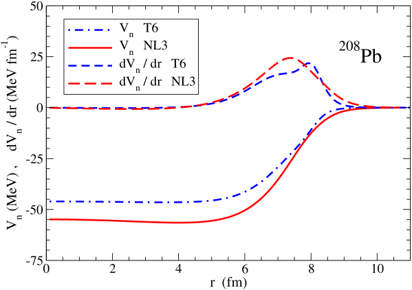
Figure 12: (Color online) Neutron single-particle potential and its derivative for the nucleus ²⁰⁸Pb obtained with the T6 Skyrme interaction in ETF2 and with the relativistic NL3 parameter set in TF approximation.

Let us try to find some reason for this deficiency and eventually a cure. What is different between the external and self consistent potential cases? The only convincing difference we can imagine is the fact that in the external potential case the density is a functional of an external fixed potential $V$, i.e. $\rho=\rho[V]$ which is expanded in powers of $\hbar$, that is in gradients of $V$. In the self consistent case the potential itself is a functional of the density and therefore also the potential has then to be expanded in a power series of $\hbar$ (we did not explicitly proceed in this way, but implicitly that is what it amounts to in the VWK method). This double $\hbar$-expansion is very likely one of the reasons for the deterioration of the results with respect to the external potential case. The WK expansion of the density matrix is a local expansion in terms of distributions functions what probably does too much harm to the self consistent potential. Some global features should be kept, even for the average potential. For example, if we were given a self consistently averaged Strutinsky HF potential, we would believe from our past experience that when it is taken as an external potential in the evaluation of the semiclassical WK-HF energy this should give very precisely the true Strutinsky averaged value of $E/A$. Of course, this would be an extremely laborious detour. One can think of employing an approximate substitute of the Strutinsky potential. A possibility is to take the self consistent potential evaluated in the ETF2 approach, instead. Indeed, as we mentioned earlier, in the ETF2 approach the density contains powers in $\hbar$ which are partially resummed to all orders in the self consistent calculation SV . Therefore, the corresponding single-particle potential, which is a well behaved smooth average potential (see Fig.12), also contains some global properties.

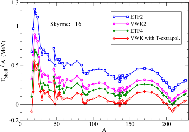
Figure 9: (Color online) Shell energies per nucleon along the $\beta$-stability line computed with the Skyrme force T6 in several approaches, including the empirical temperature extrapolation method described in Appendix 2.

We will apply this strategy to obtain another semiclassical estimate of the HF energy. To this end we first run a self-consistent ETF2 calculation with the T6 force. Next, we take the computed ETF2 mean field potential, including its spin-orbit and Coulomb contributions, as if it were an external potential and with it we perform a WK2 calculation to obtain the Skyrme energy, by using the WK expressions for particle and kinetic energy densities including $\hbar^{2}$ corrections RS . In this procedure, which clearly differs from the VWK method, some divergences arise in the evaluation of some $\hbar^{2}$ contributions (see Appendix 1 for the treatment of the divergence of the term $(\nabla\rho_{\rm WK})^{2}$ in the Skyrme energy density). To circumvent this technical difficulty, a finite temperature WK calculation is performed BGH ; VG which is extrapolated to $T=0$. The details of this method to estimate the semiclassical HF energy are described in Appendix 2. The results obtained for the shell correction per particle calculated for $\beta$-stable nuclei are shown in Fig.9 (curve labelled by “temperature extrapolation”). We see that there is a substantial improvement over the VWK2 and ETF4 results. The cure is not 100% though and there remains the fact that ⁴⁰Ca is slightly more bound semiclassically than quantally. However, globally, the average $A$-dependence of $E/A$ is now quite acceptable in particular towards the heavier nuclei. For example the shell correction for ²⁰⁸Pb is now $\sim 20$ MeV, well in line with the value reported from Strutinsky calculations with the Gogny D1S and RMF NL3 effective nuclear interactions Pom . We agree that the procedure is ad hoc; however, it helps to shed some light on the situation.

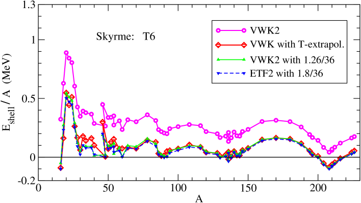
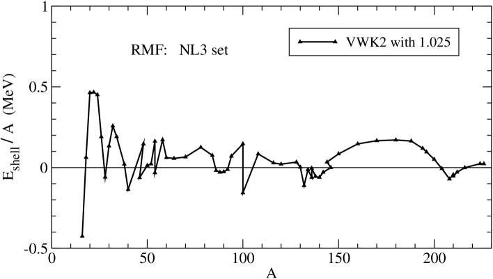
Figure 10: (Color online) Upper panel: shell energies per nucleon along the $\beta$-stability line for spherical nuclei computed with the Skyrme force T6 using the VWK2 approach and the different empirical methods described in the text. Lower panel: same for the RMF parameter set NL3. In this case the doubly magic, non $\beta$-stable nuclei ¹⁰⁰Sn and ¹³²Sn have been added for more complete information.

It is interesting to note that the WK-HF results in Fig.9 obtained with the ETF2 potential can almost perfectly be reproduced within the VWK2 method with a fudge factor on the VWK2 kinetic energy in the following way: in Eq.(12) we replace the factor 1/36 in front of the Weizsäcker term by 1.26/36 in order to increase the kinetic energy, i.e. to decrease the binding. The same result can be obtained with ETF2 by replacing 1/36 by 1.8/36 (modifications of the value of the coefficient of the Weizsäcker term have been studied in the literature since a long time ago, see e.g. Ref.KT ). We show these results for the T6 force in the upper panel of Fig.10 and find that all these different prescriptions practically lead to shell correction values on top of one another. The reason for this very close agreement, found using different prescriptions to estimate the shell corrections, is at present unknown, but it is a surprising and interesting feature.

Still we would like to deepen somewhat the discussion of the situation and of the possible reasons for the failure of VWK2 (and ETF4) to correctly reproduce the average. As mentioned above, the implicit expansion of the average mean field in powers of $\hbar$ may be the main direct reason. However, the very short range character of the nuclear force may reinforce the problem at least in the non relativistic case. For Skyrme forces the zero range character entails an unphysical shape of the self consistent TF potential. This can best be studied in half infinite nuclear matter where the self consistent TF density can be obtained in an analytic way by quadratures in the case of Skyrme forces CVDSE ; VCDS . The TF density $\rho_{0}(z)$ and the corresponding single-particle potential for a Skyrme force with $m^{*}=m$

$$V(z)=2a_{0}\rho_{0}(z)+(2+\alpha)a_{3}{\rho_{0}(z)}^{1+\alpha}-2a_{12}\,\rho^{\prime\prime}_{0}(z),$$ (29)

are displayed in Fig.11. The TF density close to the turning point, chosen at $z=0$, behaves like $\lim_{z\to 0}\rho_{0}\approx z^{2}$ and the single-particle potential $V(z)$ reaches the classical turning point at $z=0$ with zero slope. This feature is not very well seen in Fig.11 because it turns out that the bending into the horizontal tangent only happens extremly close to the classical turning point. On the other hand, such pathological behaviour is absent in the relativistic mean field approach, since the forces are of finite range. In this case the TF potential has a WS like shape and is continuous in whole space. This is shown in Fig.12 where we display the TF neutron self consistent potential for ²⁰⁸Pb obtained with the NL3 parameter set. We see that this potential has a very acceptable shape, not much different from the usual phenomenological WS potentials with about a 2 fm wide fall off width. Also the derivative of this potential is in no way anywhere more pronounced than the one corresponding to phenomenological potentials (see Fig.12). From this fact we understand that, with respect to the non-relativistic case of Skyrme forces, the semiclassical results are considerably better in the relativistic case (see Table 2 and Figs.8 and 9). At least practically all doubly magic nuclei are more bound quantally than semiclassically. However, for example for ²⁰⁸Pb the shell energy turns out to be $E_{shell}\approx 6$ MeV, a value which is about a factor 3 times too small with regard to commonly accepted values Pom ; BQ ; BQ1 . Again this problem may be attributed to this double expansion in gradients of the mean field potential and the potential itself and, as already mentioned, it cannot be excluded that the $\hbar$-expansion converges in the self consistent case more slowly than in the the external potential case. At any rate, contrary to the situation with the Skyrme forces, in the relativistic case, as already stated, the TF mean field potentials are perfectly smooth and well behaved and can, therefore, not be incriminated. At the present moment it is unclear how to remedy this situation, other than by prescriptions such as the ones presented above. However, even this must still be refined in order to become entirely realistic.

A last comment may be in order at this point. We remark in Fig.10 that for ²⁰⁸Pb the shell correction predicted by the ad-hoc methods is quite acceptable. However, there is a continuous deterioration of the situation towards lighter nuclei. Such a deterioration can in fact also be seen in Fig.8 for the SkM^∗ force and in Fig.9 for the T6 force, whereas in the relativistic case (lower panel of Fig.8) the predictions for light nuclei are more robust. For instance, both SkM* and T6 yield (wrongly) a positive shell correction energy of about 12 MeV for ⁴⁰Ca in VWK2, while NL3 at least predicts a negative value of $-2$ MeV for this nucleus (see Table 2). One possible explanation for this different behaviour could be the different treatment of the spin-orbit potential in both cases. In the non-relativistic case one should realize that the spin-orbit is not only expanded in powers of $\hbar$ but in addition one assumes the smallness of the coupling constant and only the lowest order term is taken into account. In reality the spin-orbit is a matrix problem as recognized by Frisk Frisk and then no expansion in the coupling constant is needed. To our knowledge, the validity in the expansion of the coupling constant has never been checked. On the other hand in the relativistic case such an expansion is absent, and the coupling of the spin-orbit is treated at all the orders even in the semiclassical approach CVBS . It is an open hypothesis whether this difference can explain the different behaviour in the upper and lower panels of Fig.8. The spin-orbit potential yields a surface contribution and this could point to the fact why in one case things deteriorate towards lower mass nuclei whereas in the other not. More studies on this issue are needed.

On the above grounds, it seemed interesting to us to also apply a fudge factor to the kinetic energy in the relativistic case. With the very small coefficient 1.025 we obtain the results shown in the lower panel of Fig.10. Now the shell energy of ⁴⁰Ca is 5.6 MeV and the one of ²⁰⁸Pb is 15 MeV. Both results are compatible with previously known values Pom ; BQ ; BQ1 . We therefore have now at hand, at least in the relativistic case, an ad hoc procedure which yields reasonable shell energies throughout the periodic table. This very small correction needed in the relativistic case may hint to the point that there the $\hbar^{4}$-corrections could cure the overbinding problem with no need of a fudge factor. However, for ²⁰⁸Pb still $\sim 10$ MeV overbinding in the total energy occurs semiclassically whereas for an external potential the $\hbar^{4}$-corrections to the energy are typically $\sim 1$ MeV only RS .

The conclusion of our study therefore is that the semiclassical method based on the asymptotic expansion of the Wigner-Kirkwood type is in the self consistent case more fragile, i.e. inaccurate, than in the external potential case. This failure in the case of finite nuclei is in agreement with our earlier studies on the surface energies SV ; CVDSE ; ECV which also turn out to be much more accurate in the external potential case than in the self consistent one. These findings are, however, sensitively more pronounced in the case of Skyrme forces than in the case of relativistic mean field theory.

V Conclusions

In this paper we took up again the old problem of the Thomas-Fermi approach to nuclei with incorporation of $\hbar$-corrections. As we have pointed out in earlier work SV , the well established ETF scheme, lacking a correct sorting out of powers in $\hbar$, may show unnecessary slow convergence properties. We therefore established a rigorous order by order $\hbar$ expansion of the self consistent nuclear mean field problem which we named variational-Wigner Kirkwood (VWK) theory. We here apply it for the first time to finite nuclei in realistic self consistent mean fields at order $\hbar^{2}$ (VWK2), supposing that the $\hbar^{4}$-corrections be very small, similarly to what is documented for the external potential case since several decades RS .

One essential finding of our investigation is that practically for all Skyrme forces VWK2 yields binding energies per particle very close to fourth order ETF functional theory (ETF4). This result is good and bad at the same time. The good point is that the results from ETF4 can be reproduced with the much simpler VWK2 approach and that the agreement gives further credit to the correctness of the semiclassical values. The bad side is that it is known since long BGH ; CPVGB ; PS ; Li ; BB ; CVBS ; CV ; Kumar ; BCKT that ETF even at order $\hbar^{4}$ produces E/A values with too much binding yielding for instance for doubly magic nuclei (e.g. ⁴⁰Ca or ²⁰⁸Pb) values which are lower in energy than the ones obtained from quantal Hartree-Fock calculations. Evidently this overbinding problem is then also present in VWK2.

We advanced several arguments in regard to the overbinding problem such as the zero range character of the Skyrme forces, leading to unphysical shapes of the self consistent Thomas-Fermi mean field potential, and/or an insufficient treatment of the spin-orbit potential. Those arguments are backed by the fact that in the relativistic RMF, with finite range meson exchange potentials, the situation is considerably better. Indeed in that case at least practically all of the doubly magic nuclei are more bound quantally than semiclassically. This could stem from the fact that there the Thomas-Fermi mean field potential is perfectly smooth resembling very much a realistic Woods-Saxon type of potential. Also the spin-orbit is treated properly. However, the shell corrections, e.g. for ²⁰⁸Pb, are with relativistic VWK2 (no ETF4 exists in that case) still roughly a factor of three too small. This remaining failure could have as origin that in the self consistent case, contrary to the external potential case, the mean field is itself a functional of the density and has to undergo an $\hbar$-expansion (this remark is also true in the non-relativistic case). Evidently also missing $\hbar^{4}$-corrections can be invoked. One has to keep in mind, however, that for heavy nuclei $\hbar^{4}$-corrections are typically of order 1 MeV in the external potential case, whereas even in RMF semiclassical energies are about 10 MeV overbound. Still, a slower convergence of the $\hbar$-expansion in the self consistent case is not to be excluded.

Since $\hbar^{4}$-terms enormously complicate the theory and the numerical treatment, we refrained from studying this here, and to gain further insight we rather investigated whether the situation can be improved by ad hoc prescriptions. We report on several possibilities, where a fudge factor of 1.025 on the kinetic energy in the relativistic case gives the most satisfying results. Indeed, we show in the lower panel of Fig.10 the corresponding shell energies for spherical nuclei as a function of mass number which we believe are quite realistic throughout. Probably, if in the non-relativistic case finite range forces were used, the situation also would improve there and an approach like in Ref.Swia including $\hbar^{2}$-corrections could be undertaken. However, even the Thomas-Fermi solution with the Gogny force shows pathologies, since it still contains zero range pieces. We also should mention that for simplicity our studies were done almost exclusively for spherical nuclei.

A result on the side, obtained in the external potential case, was that for spherical nuclei the semiclassical binding energies per particle as a function of particle number do not pass through the average of the quantal results. Rather the semiclassical curve (see Fig.3) shows more binding than the average. This fact, though not unknown Leb , has not been mentioned much in the past. This natural tendency of the semiclassical results to give in the spherical case (for the deformed one, see Fig.3 and remarks towards the end of Section III) more binding than the average should, however, not be confused with the overbinding problem encountered in the self consistent semiclassical approach as discussed above and in section IV.B. This is an additional and erroneous binding contribution contained in the present semiclassical expressions which brings in the self consistent case semiclassical binding energies below the ones of doubly magic nuclei, in contradiction with results from self consistent Strutinsky calculations where this is not the case and which should be the gauge for semiclassical results.

Our studies may have relevance not only for nuclear systems but also for atomic physics calculations and for all other inhomogeneous and/or self-bound Fermi systems like ³He drops, trapped cold atoms, metallic clusters, quantum dots, etc., where the application of statistical Thomas-Fermi methods is particularly helpful and valuable.

VI Acknowledgments

The authors are indebted to R.K. Bhaduri, O. Bohigas, P. Leboeuf, and W.J. Swiatecki for useful comments and informations. Especially we thank P. Leboeuf for pointing out to us that the fluctuating part of the energy in (24) contains a non-vanishing contribution when averaged over particle number and that this feature is worked out in Ref. Leb . This work has been partially supported by the IN2P3-CICYT collaboration. Two of us (X.V. and M.C.) also acknowledge financial support from Grants No. FIS2005-03142 from MEC (Spain) and FEDER, and No. 2005SGR-00343 from Generalitat de Catalunya.

VII Appendix 1

As is well known the WK $\hbar$-expansion of the particle density involves divergent terms at the classical turning point of the kind $\propto(\mu-V)^{-n/2}$ where $n$ is an odd integer and positive number, $V(\vec{r})$ the external mean field potential, and $\mu$ the chemical potential. It is well documented in the literature RS ; KCM how to deal with this divergent part and to extract the non divergent contribution of the corresponding integral. Actually, we gave in Section 3 a recipe for solving this problem in the case of an external potential. Another way consists in writing

$$(\mu-V)^{-n/2}\propto\bigg{(}\frac{\partial}{\partial\mu}\bigg{)}^{n^{\prime}}(\mu-V)^{-1/2},$$ (30)

where $n^{\prime}=(n-1)/2$ and $(\mu-V)^{-1/2}$ is an integrable divergency, and the differentation can then be done after the integration has been performed.

A case which is not so well studied is the one of $\propto(\mu-V)^{-2n^{\prime}}$, i.e. terms with integer powers of $\mu-V$ in the denominator. Such terms arise for instance when some powers of the density have to be integrated. We will show here how to extract the finite part of such integrals. In particular in the Skyrme energy computed at the WK-$\hbar^{2}$ level we have to find the integral of the following expression (see Eq.(41) of Appendix 2):

$$(\nabla\rho_{\rm WK})^{2}=I_{0}+I_{2}$$ (31)

with

$$I_{0}=C^{2}\bigg{[}\frac{9}{4}(\mu-V)\big{(}\nabla V)^{2}+\frac{3\hbar^{2}}{16m}\nabla\big{(}\Delta V\big{)}\nabla V\bigg{]}$$ (32)

the non-diverging part and

$$I_{2}=C^{2}\frac{3\hbar^{2}}{64m}\bigg{[}\frac{\nabla V\nabla\big{(}\nabla V\big{)}^{2}+2\Delta V\big{(}\nabla V\big{)}^{2}}{\mu-V}+\frac{3}{2}\frac{\big{(}\nabla V\big{)}^{2}}{(\mu-V)^{2}}\bigg{]}$$ (33)

the diverging one ($C$ is a constant). Without loss of generality we can assume here the spherically symmetric case and then we can write for the integral of (33) $i=i_{1}+i_{2}$ with

$$i_{1}=B_{1}\int^{r_{c}}_{0}drr^{2}\frac{G_{1}(r)}{\mu-V}$$ (34)

$$i_{2}=B_{2}\int^{r_{c}}_{0}drr^{2}\frac{G_{2}(r)}{(\mu-V)^{2}}$$ (35)

where $B_{1},B_{2}$ and $G_{1}$, $G_{2}$ are well defined constants and functions, respectively.

A judicious and frequently used strategy to isolate the finite contribution is to integrate by parts and disregard the diverging integrated piece. We have

$$\frac{\partial}{\partial r}\frac{1}{\mu-V}=\frac{V^{\prime}}{(\mu-V)^{2}}\,;\qquad V^{\prime}=\frac{\partial V}{\partial r}.$$ (36)

Then we can write for the integral of $I_{2}$:

$$i_{1}+i_{2}=\int^{r_{c}}_{0}dr\frac{B_{1}{\tilde{G}}_{1}-B_{2}{{\tilde{G}}_{2}}^{\prime}}{\mu-V}=i,$$ (37)

where ${\tilde{G}}_{1}=r^{2}G_{1}$ and ${\tilde{G}}_{2}=r^{2}G_{2}/V^{\prime}$. We perform one further partial integration and write, with $x=r/r_{c}$,

$$\frac{\partial}{\partial x}\ln(1-V/\mu)=-\frac{1}{\mu-V}\,\frac{\partial V}{\partial x}.$$

Again neglecting the integrated part one obtains

$$i=r_{c}\int^{1}_{0}dx\frac{\partial F}{\partial x}\,\ln(1-V/\mu),$$ (38)

where

$$F(x)=\big{[}B_{1}{\tilde{G}}_{1}-B_{2}{{\tilde{G}}_{2}}^{\prime}\big{]}\frac{1}{\partial V/\partial x}.$$ (39)

For example, for a Woods-Saxon potential the integral in Eq.(38) can directly be performed numerically. In the case of a harmonic oscillator potential $V=ar^{2}$ the integral can be performed analytically:

$$i=\gamma\big{[}\ln 2-\frac{4}{3}\big{]},$$ (40)

with

$$\gamma=\frac{3}{16}\frac{\hbar^{2}}{m}A^{2}a^{2}r^{3}_{c}.$$

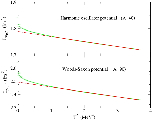
Figure 13: (Color online) Extrapolation to $T=0$ of the WK value of $\int(\nabla\rho)^{2}d\vec{r}$ obtained from HO (upper panel) and WS (lower panel) potentials.

The above result is the value which is obtained looking up integral tables. We now want to check the value of $i$ with a second independent method. This can be done writing the integral $i$ at finite temperature (see Appendix 2), where it is not divergent, and evaluating it as a function of $T$. At the end an extrapolation to $T=0$ is performed. This method is also well documented in the literature BGH and will be briefly discussed in Appendix 2 for the sake of completeness. However, the extrapolation process needs some care and usually the final number will only be precise to a couple of percent. Fig.13 displays, as a function of temperature, the value of $\int(\nabla\rho)^{2}d\vec{r}$ obtained with a HO potential (upper panel) for $A=40$ and a WS potential (lower panel) for $A=90$. As it is discussed in Appendix 2, the linear behaviour of this integral with $T^{2}$ breaks down about $T=1$ MeV (as shown by the curves that bend upwards in Fig.13), and the extrapolation to $T=0$ MeV (dashed lines of Fig.13) is needed. We find that the extrapolated values are 1.789 fm^-5 and 2.494 fm^-5 for the HO and WS potentials respectively. The values calculated with (38) give 1.867 fm^-5 (HO) and 2.383 fm^-5 (WS), which correspond to relative differences of 4.2% and 7.4%, respectively. Such errors are to be expected in the extrapolation procedure.

VIII Appendix 2

In this Appendix we present the details of the method which has been used to obtain the results displayed by the semiclassical “temperature extrapolation” curve in Fig. 9 of Sect. IV.B. It is based on a calculation of the WK-HF energy including $\hbar^{2}$ corrections that is built on top of a previously computed smooth mean field potential. The smooth potential, including the spin-orbit ($\vec{W}$) and Coulomb ($V_{\rm Coul}$) contributions, is generated in a self consistent ETF2 calculation with the Skyrme T6 interaction. It is then used as input for the WK calculation, where it is treated as an external potential. To circumvent the divergence problems (see Appendix 1) in some $\hbar^{2}$ terms of the WK-HF energy functional, we compute the energy at finite temperature and take its limit (numerically) when $T\to 0$. This has been shown in the past VG to be a very efficient procedure to overcome the divergences.

The expression of the WK energy in the case of a Skyrme force with $m^{*}=m$, including Coulomb and spin-orbit contributions, reads

$$E_{{\rm WK}} = \int d\vec{r}\bigg{\{}\frac{\hbar^{2}}{2m_{n}}\bigg{[}\frac{3}{5}\big{(}\frac{3\pi^{2}}{2}\big{)}^{2/3}\rho_{{\rm WK},n}^{5/3}+\frac{1}{36}\frac{(\nabla\rho_{{\rm WK},n})^{2}}{\rho_{{\rm WK},n}}+\frac{1}{3}\Delta\rho_{{\rm WK},n}\bigg{]}$$ (41)

$$+ \frac{\hbar^{2}}{2m_{p}}\bigg{[}\frac{3}{5}\big{(}\frac{3\pi^{2}}{2}\big{)}^{2/3}\rho_{{\rm WK},p}^{5/3}+\frac{1}{36}\frac{(\nabla\rho_{{\rm WK},p})^{2}}{\rho_{{\rm WK},p}}+\frac{1}{3}\Delta\rho_{{\rm WK},p}\bigg{]}$$

$$+ \frac{1}{2}t_{0}\bigg{[}\big{(}1+\frac{x_{0}}{2}\big{)}\rho_{{\rm WK}}^{2}-\big{(}x_{0}+\frac{1}{2}\big{)}\big{(}\rho_{{\rm WK},n}^{2}+\rho_{{\rm WK},p}^{2}\big{)}\bigg{]}$$

$$+ \frac{1}{12}t_{3}\rho_{{\rm WK}}^{\alpha}\bigg{[}\big{(}1+\frac{x_{3}}{2}\big{)}\rho_{{\rm WK}}^{2}-\big{(}x_{3}+\frac{1}{2}\big{)}\big{(}\rho_{{\rm WK},n}^{2}+\rho_{{\rm WK},p}^{2}\big{)}\bigg{]}$$

$$+ \frac{1}{16}\bigg{[}3t_{1}\big{(}1+\frac{x_{1}}{2}\big{)}-t_{2}\big{(}1+\frac{x_{2}}{2}\big{)}\bigg{]}\big{(}\nabla\rho_{{\rm WK}}\big{)}^{2}$$

$$- \frac{1}{16}\bigg{[}3t_{1}\big{(}x_{1}+\frac{1}{2}\big{)}-t_{2}\big{(}x_{2}+\frac{1}{2}\big{)}\bigg{]}\bigg{[}\big{(}\nabla\rho_{{\rm WK},n}\big{)}^{2}+\big{(}\nabla\rho_{{\rm WK},p}\big{)}^{2}\bigg{]}$$

$$+ \frac{1}{2}W_{0}\bigg{[}\vec{J}_{{\rm WK}}\cdot{\nabla\rho_{{\rm WK}}}+\vec{J}_{{\rm WK},n}\cdot{\nabla\rho_{{\rm WK},n}}+\vec{J}_{{\rm WK},p}\cdot{\nabla\rho_{{\rm WK},p}}\bigg{]}+{\cal{H}}_{\rm Coul}\bigg{\}}.$$

In this equation $\rho_{{\rm WK},q}$ ($q=n,p$) is the WK neutron or proton density including $\hbar^{2}$ corrections RS , and $\rho_{{\rm WK}}=\rho_{{\rm WK},n}+\rho_{{\rm WK},p}$. The neutron or proton semiclassical spin-current density up to $\hbar^{2}$ order is given by GV ; BGH

$$\vec{J}_{{\rm WK},q}=-\frac{2m_{q}}{\hbar^{2}}\rho^{0}_{{\rm WK},q}\vec{W}_{q},$$ (42)

where $\rho^{0}_{{\rm WK},q}$ is the TF ($\hbar^{0}$ part) of the WK neutron or proton densities, $\vec{W}_{q}$ is the (external ETF2) spin-orbit potential, and $\vec{J}_{{\rm WK}}=\vec{J}_{{\rm WK},n}+\vec{J}_{{\rm WK},p}$. The semiclassical Coulomb energy density appearing in Eq.(41) is computed as

$${\cal{H}}_{\rm Coul}=\frac{1}{2}e^{2}\rho_{{\rm WK},p}V_{\rm Coul}-\frac{3}{4}\bigg{(}\frac{3}{\pi}\bigg{)}^{1/3}e^{2}\rho_{{\rm WK},p}^{4/3}\,,$$ (43)

where $V_{\rm Coul}$ is the Coulomb potential provided by the self consistent ETF2 calculation.

At a finite temperature the relevant thermodynamical potential which has to be minimized is the free energy $F$, instead of the energy $E$. The free energy, the energy, and the entropy $S$ are related through

$$F=E-TS.$$ (44)

In the WK approach $E$ is given by Eq.(41) and the particle and kinetic energy densities at finite temperature, for (external ETF2) nuclear $V_{q}$ and spin-orbit $W_{q}$ potentials, for each kind of particle, read as BGH ; VG

$$\rho_{{\rm WK},q}^{T} = \frac{1}{2\pi^{2}}\bigg{(}\frac{2mT}{\hbar^{2}}\bigg{)}^{3/2}\bigg{\{}J_{1/2}(\eta_{q})+\frac{\hbar^{2}}{48m}\bigg{[}\frac{\Delta V_{q}}{T^{2}}J_{-3/2}(\eta_{q})+\frac{3}{4}\frac{(\nabla V_{q})^{2}}{T^{3}}J_{-5/2}(\eta_{q})\bigg{]}$$ (45)

$$+ \frac{mW_{q}^{2}}{2\hbar^{2}T}J_{-1/2}(\eta_{q})\bigg{\}}$$

and

$$\tau_{{\rm WK},q}^{T} = \frac{1}{2\pi^{2}}\bigg{(}\frac{2mT}{\hbar^{2}}\bigg{)}^{5/2}\bigg{\{}J_{3/2}(\eta_{q})-\frac{\hbar^{2}}{48m}\bigg{[}5\frac{\Delta V_{q}}{T^{3}}J_{-1/2}(\eta_{q})+\frac{9}{4}\frac{(\nabla V_{q})^{2}}{T^{3}}J_{-3/2}(\eta_{q})\bigg{]}$$ (46)

$$+ \frac{5mW_{q}^{2}}{2\hbar^{2}T}J_{1/2}(\eta_{q})\bigg{\}},$$

where $J_{\nu}(\eta_{q})$ are the so-called Fermi integrals

$$J_{\nu}(\eta_{q})=\int^{\infty}_{0}dx\,\frac{x^{\nu}}{1+\exp(x-\eta_{q})}$$ (47)

and $\eta_{q}=(\mu_{q}-V_{q})/T$ is the fugacity parameter. In particular, the free energy $F$ for a free Fermi gas moving in single-particle and spin-orbit potentials is given by

$$F_{{\rm free},q} = \mu_{q}A_{q}-\frac{1}{2\pi^{2}}\bigg{(}\frac{2mT}{\hbar^{2}}\bigg{)}^{3/2}\int\bigg{\{}d\vec{r}\frac{2}{3}TJ_{3/2}(\eta_{q})$$ (48)

$$- \frac{\hbar^{2}}{24m}\bigg{[}\frac{\Delta V_{q}}{T}J_{-1/2}(\eta_{q})+\frac{1}{4}\frac{(\nabla V_{q})^{2}}{T^{2}}J_{-3/2}(\eta_{q})\bigg{]}+\frac{mW_{q}^{2}}{\hbar^{2}}J_{1/2}(\eta_{q})\bigg{\}},$$

where $\mu_{q}$ and $A_{q}$ are the chemical potential and the particle number of each kind of nucleon. The final expression of the total free energy contains in addition to (48) the interacting potential part of the Skyrme-WK energy (41). The contributions of the powers of the particle density and its gradients in Eq. (41) are expanded in a Taylor series starting from the expression (45) and only the linear terms in $\hbar^{2}$ are retained.

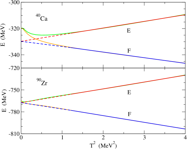
Figure 14: (Color online) Extrapolation to $T=0$ of the Skyrme energy ($E$) and free energy ($F$) corresponding to the T6 force obtained with the thermal WK method on top of the self consistent ETF2 potential for ⁴⁰Ca (upper panel) and ⁹⁰Zr (lower panel).

The ETF2 potentials used in Eqs.(45), (46) and (48) are obtained at zero temperature, i.e., it is assumed that they are temperature independent. It should be pointed out that, even in a fixed external potential, the system starts to evaporate nucleons as soon as the finite temperature appears VG and one should resort to e.g. a subtraction procedure S87 to keep the integrated magnitudes finite and independent of the size of the box in which they are calculated. However, as far as we are interested in the $T\to 0$ limit of the free energy, we can safely neglect the effects from evaporated nucleons because they are negligible below $T\simeq 2$ MeV BQ . In such conditions one can consider the low-temperature expansion BT of the free energy and parametrize it below $T=2$ MeV as $F(T)=E(T=0)-a(T=0)\,T^{2}$. However, it is to be noted that the integrals of some terms of the interacting WK free energy, namely the ones coming from $(\nabla V_{q})^{2}$ and from the exchange Coulomb potential, which show a logarithmic divergence at zero temperature, start to depart from the linear behaviour with $T^{2}$ below $T=1$ MeV and bend upwards of the linear curve, similarly to what happens in Fig.13 where the particular term $\int(\nabla\rho)^{2}d\vec{r}$ is plotted as a function of $T^{2}$. Thus, we have estimated the WK energy by extrapolating the linear region in $T^{2}$ between $T=2$ and $T=1$ MeV. As an example, we display in Fig.14 the results of this procedure for the nuclei ⁴⁰Ca and ⁹⁰Zr calculated with the Skyrme T6 force for which we find $E\simeq-329.3$ and $-766.8$ MeV, respectively.

Table 1: Chemical potential $\mu$ calculated quantally and semiclassically with the TF and WK approaches [by inversion of Eq.(20)] as a function of the accumulated number of fermions occupying the $n=4$ shell in a spherical HO potential. Within this shell the quantal energy is computed adding a quantum $11\hbar\omega/2$ per fermion to the background energy obtained filling the previous HO shells. The semiclassical energies are obtained from Eq.(21). Both $\mu$ and $E$ are in $\hbar\omega$ units. Spin degeneracy of each level is assumed.

N	$\mu$(QM)	$\mu$(TF)	$\mu$(WK)	E(QM)	E(TF)	E(WK)
42	5.5	5.013	5.063	161.	157.919	161.092
44	5.5	5.092	5.141	172.	168.024	171.296
46	5.5	5.168	5.216	183.	178.284	181.653
48	5.5	5.241	5.289	194.	188.693	192.159
50	5.5	5.313	5.360	205.	199.248	202.809
52	5.5	5.383	5.430	216.	209.945	213.599
54	5.5	5.451	5.497	227.	220.780	224.526
56	5.5	5.518	5.563	238.	231.750	235.587
58	5.5	5.583	5.628	249.	242.851	246.778
60	5.5	5.646	5.690	260.	254.080	258.096
62	5.5	5.708	5.752	271.	265.434	269.539
64	5.5	5.769	5.812	282.	276.912	281.103
66	5.5	5.828	5.871	293.	288.510	292.787
68	5.5	5.887	5.929	304.	300.225	304.588
70	5.5	5.943	5.986	315.	312.056	316.504

Table 2: Total energies per nucleon of some magic nuclei obtained with the SkM^∗ and T6 Skyrme interactions and with the NL3 relativistic mean field parameter set in several approaches. The Coulomb and spin-orbit forces are included in the calculations. The column VWK-T refers to the empirical “temperature extrapolation” method described in Appendix 2.

		SkM∗	SkM∗	T6	T6	T6	NL3	NL3
	A	HF	VWK	HF	VWK	VWK-T	H	VWK
	16	$-$7.081	$-$7.309	$-$7.026	$-$7.348	$-$6.934	$-$7.282	$-$6.965
	40	$-$8.126	$-$8.447	$-$8.141	$-$8.428	$-$8.243	$-$8.315	$-$8.265
	48	$-$8.387	$-$8.565	$-$8.332	$-$8.596	$-$8.336	$-$8.461	$-$8.463
	90	$-$8.502	$-$8.659	$-$8.514	$-$8.719	$-$8.527	$-$8.603	$-$8.641
	208	$-$7.779	$-$7.777	$-$7.786	$-$7.828	$-$7.701	$-$7.845	$-$7.817

Figure 11: Thomas-Fermi density (upper panel) and single-particle potential (lower panel) profiles in half infinite symmetric nuclear matter obtained using the T6 T6 force. The fact that the potential enters the classical turning point with a horizontal tangent cannot be seen on the scale of the graph.

References

- (1) T. S. H Skyrme, Philos. Mag. 1, 1043 (1956); Nucl. Phys. 9, 615 (1959); D. Vautherin and D. M. Brink, Phys. Rev. C5, 626 (1972).
- (2) J. Dechargé and D. Gogny, Phys. Rev. C21, 1568 (1980).
- (3) B. D. Serot and J. D. Walecka, Adv. Nucl. Phys. 16, 1 (1986); P.-G. Reinhard, Rep. Prog. Phys. 52, 439 (1989); P. Ring, Prog. Part. Nucl. Phys. 37, 193 (1996); B. D. Serot and J. D. Walecka, Int. J. Mod. Phys. E6, 515 (1997).
- (4) W. D. Myers, Droplet Model of Atomic Nuclei (Plenum, New York, 1977); W. D. Myers and W. J. Swiatecki, Ann. of Phys. (NY) 55, 395 (1969); Ann. of Phys. (NY) 84, 186 (1974).
- (5) V.M. Strutinsky, Nucl. Phys. A95 420 (1967); Nucl. Phys. A122 1 (1968).
- (6) R. K. Bhaduri and C. K. Ross, Phys. Rev. Lett. 27, 606 (1971); M. Brack and H. C. Pauli, Nucl. Phys. A207, 401 (1973); B. K. Jennings, Nucl. Phys. A207, 538 (1973); B. K. Jennings, R. K. Bhaduri, and M. Brack, Nucl. Phys. A253, 29 (1975).
- (7) W. D. Myers and W. J. Swiatecki, Nucl. Phys. A601, 141 (1996), and http://ie.lbl.gov/txt/ms.txt
- (8) E. Wigner, Phys. Rev. 40, 749 (1932); J. G. Kirkwood, Phys. Rev. 44, 31 (1933); G. E. Uhlenbeck and E. Beth, Physica 3, 729 (1936).
- (9) P. Ring and P. Schuck, The Nuclear Many-Body Problem (Springer-Verlag, Berlin, 1980).
- (10) H. Krivine, M. Casas, and J. Martorell, Ann. of Phys. (NY) 200, 304 (1990).
- (11) P. Schuck and X. Viñas, Phys. Lett. B302, 1 (1993).
- (12) M. Centelles, X. Viñas, M. Durand, P. Schuck and D. Von-Eiff, Ann. of Phys. (NY) 266, 207 (1998).
- (13) M. Del Estal, M. Centelles and X. Viñas, Phys. Rev. C56, 1774 (1997).
- (14) P. Hohenberg and W. Kohn, Phys. Rev. 136, B864 (1964).
- (15) B. Grammaticos and A. Voros, Ann. of Phys. (NY) 123, 359 (1979); Ann. of Phys. (NY) 129, 275 (1980).
- (16) M. Brack, C. Guet and H. B. Håkansson, Phys. Rep. 123, 275 (1985).
- (17) M. Centelles, M. Pi, X. Viñas, F. Garcias and M. Barranco, Nucl. Phys. A510, 397 (1990).
- (18) I. Zh. Petkov and M. V. Stoitsov, Nuclear Density Functional Theory (Clarendon Press, Oxford, 1991).
- (19) Li Guo-Qiang, J. of Phys. G17, 1 (1991).
- (20) M. Centelles, X. Viñas, M. Barranco and P. Schuck, Ann. of Phys. (N.Y.) 221, 165 (1993).
- (21) M. Centelles and X. Viñas, Nucl. Phys. A563, 173 (1993).
- (22) M. Brack and R. K. Bhaduri, Semiclassical Physics (Addison-Wesley, Reading, MA, 1997).
- (23) M. Centelles, M. Del Estal and X. Viñas, Nucl. Phys. A 635, 193 (1998).
- (24) V. B. Soubbotin and X. Viñas, Nucl. Phys. A 665, 291 (2000).
- (25) M. Centelles, P. Schuck, X. Viñas, and P. Leboeuf, to be published.
- (26) M. Brack and S. R. Jain, Phys. Rev. A51, 3462 (1995).
- (27) B. K. Jennings, R. K. Bhaduri and M. Brack, Phys. Rev. Lett. 34, 228 (1975).
- (28) S. Shlomo, Nucl. Phys. A539, 17 (1992).
- (29) W. Nazarewicz, T. R. Werner and J. Dobaczewski, Phys. Rev. C50, 2860 (1994).
- (30) T. Verste, A. T. Kruppa, R. J. Liotta, W. Nazarewicz, N. Sandulescu and T. R. Werner, Phys. Rev. C57, 3089 (1998).
-
(31)
A. G. Monastra, PhD thesis 2001, Fluctuations quantiques dans les
systèmes fermioniques de taille finie, Université Paris XI, UFR
Scientifique d’Orsay, http://www.physik.tu-dresden.de/
~monastra - (32) K. Pomorski, Phys. Rev. C70, 044306 (2004).
- (33) M. Rayet, M. Arnould, F. Tondeur and G. Paulus, Astron. Astrophys. 116, 183 (1982).
- (34) M. Beiner, H. Flocard, Nguyen Van Giai, and P. Quentin, Nucl. Phys. A238, 29 (1975).
- (35) M. Centelles, X. Viñas, M. Barranco, S. Marcos and R. J. Lombard, Nucl. Phys. A537, 486 (1992).
- (36) M. Kleban, B. Nerlo-Pomorska, J.F. Berger, J. Dechargé, M. Girod and S. Hilaire, Phys. Rev. C65, 024309 (2002); B. Nerlo-Pomorska and K. Mazurek, Phys. Rev. C66, 064305 (2002).
- (37) M. Brack and P. Quentin, Phys. Lett. 52 B, 159 (1974).
- (38) M. Brack and P. Quentin, Phys. Lett. 56 B 421 (1975); Nucl. Phys. A361, 35 (1981).
- (39) P. Moller, J. R. Nix and K.-L. Kratz, At. Data Nuc. Data Tables 66, 131 (1997).
- (40) P. Moller, J. R. Nix, W. D. Myers and W. J. Swiatecki, At. Data Nucl. Data Tables 59, 185 (1995).
- (41) G.A. Lalazissis, J. Köning and P. Ring, Phys. Rev. C55, 540 (1997).
- (42) K. Kumar and R. K. Bhaduri, Phys. Rev. 122, 1926 (1961).
- (43) O. Bohigas, X. Campi, H. Krivine, and J. Treiner, Phys. Lett. B64, 381 (1976).
- (44) N. H. March, Self-consistent Fields in Atoms, (Pergamon, Oxford, 1975).
- (45) H. Krivine and J. Treiner, Phys. Lett. 88B, 212 (1979).
- (46) X. Viñas, M. Centelles, M. Durand and P. Schuck, in Proceedings of the International Conference on Many-Body Physics, Coimbra, 19993, edited by C. Fiolhais et al. (World Scientific, Singapore, 1994), p.383.
- (47) H. Frisk and T. Guhr, Ann. of Phys. (N.Y.) 221, 229 (1993).
- (48) X. Viñas and A. Guirao, Nucl. Phys. A467, 326 (1987).
- (49) E. Suraud, Nucl. Phys. A462, 107 (1987).
- (50) M. Barranco and J. Treiner, Nucl. Phys. A351, 269 (1981).