The physics of dense hadronic matter and compact stars

Abstract

This review describes the properties of hadronic phases of dense matter in compact stars. The theory is developed within the method of real-time Green’s functions and is applied to study of baryonic matter at and above the saturation density. The non-relativistic and covariant theories based on continuum Green’s functions and the $T$-matrix and related approximations to the self-energies are reviewed. The effects of symmetry energy, onset of hyperons and meson condensation on the properties of stellar configurations are demonstrated on specific examples. Neutrino interactions with baryonic matter are introduced within a kinetic theory. We concentrate on the classification, analysis and first principle derivation of neutrino radiation processes from unpaired and superfluid hadronic phases. We then demonstrate how neutrino radiation rates from various microscopic processes affect the macroscopic cooling of neutron stars and how the observed $X$-ray fluxes from pulsars constrain the properties of dense hadronic matter.

1 Introduction

Neutron stars are born in a gravitational collapse of luminous stars whose core mass exceeds the Chandrasekhar limit for a self-gravitating body supported by degeneracy pressure of electron gas [1]. Being the densest observable bodies in our universe they open a window on the physics of matter under extreme conditions of high densities, pressures and strong electromagnetic and gravitational fields. Most of the known pulsars are isolated objects which emit radio-waves at frequencies $10^{8}-10^{10}$ Hz, which are pulsed at the rotation frequency of the star. Young objects, like the pulsar in the Crab nebula, are also observed through $X$-rays that are emitted from their surface as the star radiates away its thermal energy. Relativistic magnetospheres of young pulsars emit detectable non-thermal optical and gamma radiation; they could be sources of high-energy elementary particles. Neutron stars in the binaries are powered by the energy of matter accreted from companion star.

The radio observations of pulsars stretch back to 1967 when the first pulsar was discovered. Since then, the observational pulsar astronomy has been extremely important to the fundamental physics and astrophysics, which is evidenced by two Nobel awards, one for the discovery of pulsars (Hewish 1974) [2], the other for the discovery of the first neutron star – neutron star binary pulsar (Hulse and Taylor, 1993) [3] whose orbital decay confirmed the gravitational radiation in full agreement with Einstein’s General Theory of Relativity. The measurements of neutron star (NS) masses in binaries provide one of the most stringent constraint on properties of the superdense matter. The timing observations of the millisecond pulsars set an upper limit on the angular momentum that can be accommodated by a stable NS - a limit that can potentially constrains the properties of dense matter. Noise and rotational anomalies that are superimposed on the otherwise highly stable rotation of these objects provide a clue to the superfluid interiors of these stars.

The orbiting $X$-ray satellites allow astronomers to explore the properties of the NS’s surface, in particular its composition through the spectrum of thermal radiation and the transients like thermonuclear burning of accreted material on the surface of an accreting NS. The currently operating Chandra $X$-ray satellite, Newton $X$-ray Multi Mirror Mission (XMM), Rossi $X$-ray timing explorer (RXTE) continue to provide new insight into compact objects, their environment and thermal histories. Confronting the theoretical models of NS cooling with the $X$-ray observations constrains the properties of dense hadronic matter, its elementary particle content and its condensed matter aspects such as superfluidity and superconductivity.

The currently operating gravitational wave observatories VIRGO, LIGO, GEO and TAMA are expected to detect gravity waves from various compact objects, the NS-NS binaries being one of the most important targets of their search. Higher sensitivity will be achieved by the future space-based observatory LISA, currently under construction. The global oscillations of isolated NS and NS in binaries with compact objects (in particular with NSs and black holes) are believed to be important sources of gravity waves, which will have the potential to shed light on the internal structure and composition of a NS.

The theory of neutron stars has its roots in the 1930s when it was realized that self-gravitating matter can support itself against gravitational collapse by the degeneracy pressure of fermions (electrons in the case of white dwarfs and neutrons and heavier baryons in the case of neutron stars). The underlying mechanism is the Pauli exclusion principle. Thus, unlike the ordinary stars, which are stabilized by their thermal pressure, neutron stars owe their very existence to the quantum nature of matter. The theory of neutron stars has been rapidly developing during the past four decades since the discovery of pulsars. The progress in this field was driven by different factors: the studies of elementary particles and their strong and weak interactions at terrestrial accelerators and the parallel developments in the fundamental theory of matter deeply affected our current understanding of neutron stars. The concepts of condensed matter, such as superfluidity and superconductivity, play a fundamental role in the dynamical manifestation of pulsars, their cooling and transport properties. Another factor is the steady increase of computational capabilities.

This review gives a survey of the many-body theory of dense matter in NS. It concentrates on the uniform phases and hadronic degrees of freedom which cover the density range $\rho_{0}\leq\rho\leq 3\rho_{0}$, where $\rho_{0}$ is the nuclear saturation density. The theory is developed within the framework of continuum Green’s function technique at finite temperature and density [4, 5, 6, 7]. Such an approach allows for a certain degree of coherence of the presentation. Subsection 2.10 at the end of Chapter 2 gives a brief summary of methods and results omitted in the discussion. It is virtually impossible to cover all the aspects of the NS theory even when restricting to a certain domain of densities and degrees of freedom. The topics included in this review are not surprisingly aligned with the research interests of the author. It should be noted that there are very good textbooks [8, 9], monographs [11, 12, 10] and recent lecture notes [13] that cover the basics of compact star theory much more completely than it is done in this review. Furthermore there are several recent comprehensive reviews that cover more specialized topics of NS theory such as the role of strangeness in compact stars [14], cooling of neutron stars [15, 16], neutrino propagation [17], phases of quark matter at high densities [18, 19, 20] and the equations of state of hadronic matter [21, 22, 23].

The remainder of this introduction gives a brief overview of phases of dense matter in neutron stars. Chapter 2 starts with an introduction to the finite temperature non-equilibrium Green’s functions theory. Further we give a detailed account of the $T$-matrix theory in the background medium and discuss the precursor effects in the vicinity of critical temperature of superfluid phase transition. Extensions of the $T$-matrix theory to describe the superfluid phases and three-body correlations are presented. A virial equation of state is derived, which includes the second and the third virial coefficients for degenerate Fermi-systems. The formal part of this Chapter includes further a discussion of the Brueckner-Bethe-Goldstone theory of nuclear matter, the covariant version of the $T$-matrix theory (known as the Dirac-Brueckner theory). We further discuss isospin asymmetric nuclear matter, onset of hyperons and meson condensates, and the conditions of charge neutrality and $\beta$-equilibrium that are maintained in compact stars. We close the chapter by a discussion of stellar models constructed from representative equations of state.

Chapter 3 discusses the weak interactions in dense matter within the covariant extension of the real-time Green’s functions formalism described in Chapter 2. We discuss the derivation of neutrino emissivities from quantum transport equations for neutrinos and the dominant processes that contribute to the neutrino cooling rates of hadronic matter. Special attention is paid to processes that occur in the superfluid phases of neutron stars.

Chapter 4 is a short overview of cooling simulations of compact stars. It contains several example simulations with an emphasis on the processes that were discussed in Chapter 3.

1.1 A brief overview of neutron star structure

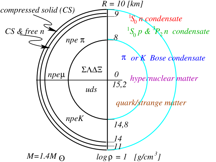
Figure 1: Schematic cross section of a $M=1.4M_{\odot}$ mass neutron star. The different stable phases and their constituents (using the standard notations) are shown as a function of the radius in the upper half of the diagram and as a function of the logarithm of the density $\rho$ in the lower half. Note that the both scales are strongly expanded in the low-density/large-radius domain. For details see the text.

We now adopt a top to bottom approach and review briefly the sequence(s) of the phases of matter in neutron stars as the density is increased. A schematic picture of the interior of a $M=1.4M_{\odot}$ mass neutron star is shown in Fig. 1. The low-density region of the star is a highly compressed fully ionized matter at densities about $\rho=10^{6}$ g cm³ composed of electrons and ions of ⁵⁶Fe. This phase could be covered by several cm thick ‘blanket’ material composed of H, He, and other light elements, their ions and/or molecules. The composition of the surface material is an important ingredient of the photon spectrum of the radiation, which is used to infer the surface photon luminosities of NS. Charge neutrality and equilibrium with respect to weak processes imply that the matter becomes neutron rich as the density is increased. In the density range $10^{7}\leq\rho\leq 10^{11}$ g cm^-3 a typical sequence of nuclei that are stable in the ground state is ⁶²Ni, ⁸⁶Kr, ⁸⁴Se, ⁸²Ge, ⁸⁰Zn, ¹²⁴Mo, ¹²²Zr, ¹²⁰Sr and their neutron rich isotopes. The matter is solid below the melting temperature $T_{m}\sim 10^{7}$ K, the electron wave functions are periodic Bloch states, and the elementary excitations are the electron quasiparticles and phonons. The lattice may also contain impurities, i. e. nuclei with mass numbers different from the predicted stable nucleus, as the time-scales for relaxation to the absolute ground state via weak interactions could be very large. The transport properties of the highly compressed solid (CS) are fundamental to the understanding of the way the thermal energy is transported from the core to the surface and the way the magnetic fields evolve in time.

Above the density $\rho\simeq 4\times 10^{11}$ g cm^-3 not all the neutrons can be bound into clusters, and those which are free to form a continuum of states fill a Fermi-surface characterized by a positive chemical potential. Thus, the “inner crust” is a CS featuring a neutron fluid. The sequence of the nuclei in the inner crust are neutron rich isotopes of Zr and Sn, with the number of protons $Z=40$ and $50$ respectively and mass number in the range $100\leq A\leq 1500$. Below the critical temperature $T_{c}\sim 10^{10}$ K, which corresponds to 1 MeV (1 MeV $=1.602\times 10^{10}$ K) neutrons in the continuum undergo a phase transition to the superfluid state. At low temperatures, the electron quasiparticles and the lattice phonons are the relevant degrees of freedom which control the thermal and magnetic properties of the matter. At non-zero temperatures neutron excitations out of condensate can play an important role in mass transport and weak neutral current processes.

At about half of the nuclear saturation density, $\rho_{0}=2.8\times 10^{14}$ g cm^-3 the clusters merge into continuum leaving behind a uniform fluid of neutrons, protons and electrons. The uniform neutron ($n$), proton ($p$) and electron ($e$) and possibly muon ($\mu$) phase extends up to densities of a few $\rho_{0}$; the $p$, $e$ and $\mu$ abundances are in the range 5-10$\%$. The many-body theory which determines the energy density of matter in this density range (as well as at higher densities) is crucial for the structure of the neutron stars, since most of the mass of the star resides above the nuclear saturation density. The neutrons and protons condense in superfluid and superconducting states below critical temperatures of the order $10^{9}$ K. Because of their low density the protons pair in the relative ${}^{1}S_{0}$ state; neutron Fermi-energies lie in the energy range where attractive interaction between neutrons is in the ${}^{3}P_{2}-^{3}F_{2}$ tensor spin-triplet channel. The relevant quasiparticle excitations of the $npe\mu$-phase are the electrons and muons at low temperatures; at moderate temperatures the neutron and proton excitations out of the condensate can be important.

The actual state of matter above the densities $2-3\times\rho_{0}$ is unknown. The various possible phases are shown in Fig 1. At a given density the largest energy scale for charge neutral and charged particles are the Fermi-energies of neutrons and electrons, respectively. Once these scales become of the order of the rest mass of strangeness carrying heavy baryons, the $\Sigma^{\pm,0}$, $\Lambda$, $\Xi^{\pm,0}$ hyperons nucleate in matter. Their abundances are again controlled by the equilibrium with respect to weak interactions and charge neutrality. Since the densities reached in the center of a massive NS are about 10$\times\rho_{0}$, it is likely that the critical deconfinment density at which the baryons lose their identity and disintegrate into up ($u$), down ($d$), and possibly strange ($s$) quarks is reached inside massive compact stars. The critical density for the deconfinement transition cannot be calculated reliably since it lies in a range where quantum chromodynamics (QCD) is non-perturbative. NS phenomenology is potentially useful for testing the conjecture of high-density cold quark matter in compact stars.

At densities $\rho\geq 2\rho_{0}$ Bose-Einstein condensates (BEC) of pions ($\pi$), kaons ($K$), and heavier mesons can arise under favorable assumptions about the effective meson-nucleon and nucleon-nucleon interactions in matter. For example, the pion condensation arises because of the instability of the particle-hole nucleonic excitations in the medium with quantum numbers of pions. This instability depends on the details of the nuclear interaction in the particle-hole channel and is uncertain. There are very distinct signatures associated with the pion and kaon BEC in the physics of NS featuring such a condensate, which includes softening of the equation of state and fast neutrino cooling.

2 The nuclear many-body problem

2.1 Real-time Green’s functions

Figure 2: The Schwinger (left) and Keldysh (right) contours; the axis corresponds to the real time, $t_{0}$ is the observation time. The time flows from left to the right on the upper branch and from right to the left on the lower branch of the contour.

Consider a non-relativistic Fermi system interacting via two-body forces. The Hamiltonian in the second quantized form is

$${\cal H}=\frac{1}{2m}\sum_{\sigma}\int d^{4}x\bm{\nabla}\psi_{\sigma}^{\dagger}(x)\bm{\nabla}\psi_{\sigma}(x)+\frac{1}{2}\sum_{\sigma\sigma^{\prime}}\int d^{4}xd^{4}x^{\prime}\psi_{\sigma}^{\dagger}(x)\psi_{\sigma^{\prime}}^{\dagger}(x^{\prime})V_{\sigma,\sigma^{\prime}}(x,x^{\prime})\psi_{\sigma^{\prime}}(x^{\prime})\psi_{\sigma}(x),$$ (1)

where $\psi_{\sigma}(x)$ are the Heisenberg field operators, $x=(\bm{r},t)$ is the space-time four vector, $\sigma$ stands for the internal degrees of freedom (spin, isospin, etc.), $m$ is the fermion mass and $V(x,x^{\prime})$ is the interaction potential, which we assume to be local in time $V(x,x^{\prime})=V(\bm{r},\bm{r}^{\prime})\delta(t-t^{\prime})$. The creation and annihilation operators obey the fermionic anti-commutation rules, $\{\psi_{\sigma^{\prime}}(x^{\prime}),\psi_{\sigma}^{\dagger}(x)\}=\delta(x-x^{\prime})$ and $\{\psi_{\sigma^{\prime}}(x^{\prime}),\psi_{\sigma}(x)\}=0$, and their equation of motion is given by $i\partial_{t}\psi(x)=\left[\psi(x),{\cal H}\right],$ where $[,]$ and $\{,\}$ stand for a commutator and anti-commutator (here and below $\hbar=c=1$). The fundamental object of the theory is the path-ordered correlation function

$${\bm{G}}(1,1^{\prime})=-i\langle{\cal P}\psi(1)\psi^{\dagger}(1^{\prime})\rangle,$$ (2)

where the path-ordering operator arranges the fields along the contour such that that time arguments of the operators increase from left to right as one moves along the contour shown in Fig. 2 (here and below the boldface characters stand for functions that are ordered on the contour). The unitary time evolution operator propagates the fermionic wave function according to $\psi(t_{2})=\hat{S}(t_{1},t_{2})\psi(t_{1})$ along the Schwinger contour from $-\infty\to t_{0}\to+\infty$, where $t_{0}$ is the observation time (Fig. 2). The Keldysh contour is obtained from the above one by inserting a piece that propagates from $t_{0}\to+\infty$ and back. The Keldysh formalism is based on a minimal extension of the usual diagrammatic rules, where depending on whether the time argument lies on the upper or lower branch of the contour a correlation function is assigned a + or – sign (per time argument). Below we follow a different path, which is based on mapping correlation function defined on the Schwinger contour on a set of alternative functions which obey tractable transport equations.

Starting from the equation of motion for the field $\psi(x)$ and its conjugate one can establish a hierarchy of coupled equations of motions for correlations functions involving increasing number of fields (in equilibrium this hierarchy is know as the Martin-Schwinger hierarchy [24]). For the single particle propagator the equation of motion is

$${\bm{G}}_{0}(1)^{-1}{\bm{G}}(1,1^{\prime})=\bm{\delta}(1-1^{\prime})-i\int_{C}d2d3d4~{}V(12;34)~{}{\bm{G}}_{2}(34,1^{\prime}2^{+}),$$ (3)

where ${\bm{G}}_{0}(1)=(i\partial_{t}+{\bm{\nabla}^{2}}/{2m}-\mu)^{-1}$ and ${\bm{G}}_{2}$ are the free single particle and the two-particle propagators, $\mu$ is the chemical potential, the notation $1^{+}\equiv(x_{1},t_{1}+0$), the time integration goes over the contour and the counter-ordered delta function is defined as $\bm{\delta}(t-t^{\prime})=\delta(t-t^{\prime})$ if $t,t^{\prime}\in C_{+}$, $\bm{\delta}(t-t^{\prime})=-\delta(t-t^{\prime})$ if $t,t^{\prime}\in C_{-}$ and $\bm{\delta}(t-t^{\prime})=0$ otherwise; here $C_{+/-}$ refer to the upper and lower branches of the contour in Fig. 2. To solve Eq. (3) we need an equation of motion for the two-particle propagator which in turn depends on the three-particle propagator and so on. The hierarchy is (formally) decoupled by defining the contour self-energy as

$${\bm{\Sigma}}(1,3){\bm{G}}(3,1^{\prime})=-i\int_{C}d2d4~{}V(12;34)~{}{\bm{G}}_{2}(34,1^{\prime}2).$$ (4)

This leads to a closed equation for the single particle propagator, which upon subtracting its complex conjugate takes the form

$$\left[{\bm{G}}^{*}_{0}(1^{\prime})-{\bm{G}}_{0}(1)\right]{\bm{G}}(1,1^{\prime})=\int_{C}d2\left[{\bm{G}}(1,2)~{}{\bm{\Sigma}}(2,1^{\prime})-{\bm{\Sigma}}(1,2)~{}{\bm{G}}(2,1^{\prime})\right].$$ (5)

If the time arguments of the contour ordered propagators are constrained to the upper/lower branches of the contour we obtain the causal/acausal propagators of the ordinary propagator time perturbation theory

$$G^{c}(1,1^{\prime})=-i\langle{\cal T}\psi(1)\psi^{\dagger}(1^{\prime})\rangle,\quad G^{a}(1,1^{\prime})=-i\langle{\cal A}\psi(1)\psi^{\dagger}(1^{\prime})\rangle,$$ (6)

where ${\cal T}$ and ${\cal A}$ are the time ordering and anti-ordering operators. The fundamental difference to the ordinary theory is the appearance of the propagators with fixed time arguments (which can be located on either branch of the contour)

$$G^{<}(1,1^{\prime})=-i\langle\psi(1)\psi^{\dagger}(1^{\prime})\rangle,\quad G^{>}(1,1^{\prime})=i\langle\psi^{\dagger}(1^{\prime})\psi(1)\rangle.$$ (7)

The propagators (6) and (7) are not independent

$$G^{c}(1,1^{\prime}) = \theta(t_{1}-t_{1}^{\prime})G^{>}(1,1^{\prime})+\theta(t_{1}^{\prime}-t_{1})G^{<}(1,1^{\prime}),$$ (8)

$$G^{a}(1,1^{\prime}) = \theta(t_{1}^{\prime}-t_{1})G^{>}(1,1^{\prime})+\theta(t_{1}-t_{1}^{\prime})G^{<}(1,1^{\prime}),$$ (9)

where $\theta(t)$ is the Heaviside step function. The equilibrium properties of the system are most easily described by the retarded and advanced propagators, which obey integral equations in equilibrium. These are defined as

$$G^{R}(1,1^{\prime}) = \theta(t_{1}-t_{1}^{\prime})[G^{>}(1,1^{\prime})-G^{<}(1,1^{\prime})],$$ (10)

$$G^{A}(1,1^{\prime}) = \theta(t_{1}^{\prime}-t_{1})[G^{<}(1,1^{\prime})-G^{>}(1,1^{\prime})].$$ (11)

There are six different self-energies associated with each propagator in Eqs. (7)-(11). The components of any two-point function defined on a time contour (in particular the single-time Green’s functions and self-energies) obey the following relations

$${\cal F}^{R}(1,1^{\prime})-{\cal F}^{A}(1,1^{\prime}) = {\cal F}^{>}(1,1^{\prime})-{\cal F}^{<}(1,1^{\prime}),$$ (12)

$${\cal F}^{R/A}(1,1^{\prime}) = \mathop{\rm Re}{\cal F}(1,1^{\prime})\pm i\mathop{\rm Im}{\cal F}(1,1^{\prime}),$$ (13)

from which, in particular, we obtain a useful relation $2i\mathop{\rm Im}{\cal F}(1,1^{\prime})={\cal F}^{>}(1,1^{\prime})-{\cal F}^{<}(1,1^{\prime}).$ In practice, systems out of equilibrium are described by the time evolution of the distribution function which, as we shall see, is related to the propagator $G^{<}(1,1^{\prime})$. The propagator $G^{>}(1,1^{\prime})$ is related to the distribution function of holes. To obtain an equation of motion for these functions from the equation of motion of the path ordered Green’s function (5) we shall use algebraic relations for a convolution of path-ordered functions,

$$C(1,1^{\prime})=\int_{C}d2A(1,2)B(2,1^{\prime}),$$ (14)

known as the Langreth-Wilkins rules [25]. These rules are stated as

$$C^{>,<}(1,1^{\prime}) = \int d2\left[A^{R}(1,2)B^{>,<}(2,1^{\prime})+A^{>,<}(1,2)B^{A}(2,1^{\prime})\right],$$ (15)

$$C^{R/A}(1,1^{\prime}) = \int d2\left[A^{R/A}(1,2)B^{R/A}(2,1^{\prime})\right].$$ (16)

Upon applying the rule (15) to Eq. (5) and using the relations (12) and (13) one obtains the Kadanoff-Baym transport equation [5]

$$\left[G_{0}^{-1}(1^{\prime})-\mathop{\rm Re}\Sigma(1,1^{\prime}),G^{<}(1^{\prime},1)\right]-\left[\mathop{\rm Re}G(1,1^{\prime}),\Sigma(1^{\prime},1)\right]$$

$$\hskip 113.81102pt=\frac{1}{2}\left\{G^{>}(1,1^{\prime}),\Sigma^{<}(1^{\prime},1)\right\}-\frac{1}{2}\left\{\Sigma^{>}(1,1^{\prime}),G^{<}(1^{\prime},1)\right\}.$$ (17)

The first term on the l. h. side of Eq. (2.1) is the counterpart of the drift term of the Boltzmann equation; the second term does not have an analog in the Boltzmann equation and vanishes in the limit where the particles are treated on the mass-shell. The r. h. side of Eq. (2.1) is the counterpart of the collision integral in the Boltzmann equation, whereby $\Sigma^{>,<}(1,1^{\prime})$ are the collision rates. An important property of the collision term is its symmetry with respect to the exchange $>~{}\leftrightarrow~{}<$, which means that the collision term is invariant under the exchange of particle and holes. Before turning to the evaluation of the self-energies we briefly outline the reduction of Eq. (2.1) to the Boltzmann’s quantum kinetic equation.

If the characteristic inter-collision distances are much greater than the inverse momenta of particles and the relaxation times are much larger than the inverse particle frequencies, quasiclassical approximations is valid. This means that the dynamics of slowly varying center-of-mass four-coordinate $x=(x_{1}+x_{2})/2$ separates from the the dynamics of rapidly varying relative coordinate $\xi=x_{1}-x_{2}$. One performs a Fourier transform with respect to the relative coordinates and expands the two-point functions with respect to (small) gradients of the slowly varying center-of-mass coordinates [26]. Upon keeping the first order gradients one obtains

$$i\{\mathop{\rm Re}G^{-1}(p,x),G^{<}(p,x)\}_{P.B.}+i\{\Sigma^{<}(p,x),\mathop{\rm Re}G(p,x)\}_{P.B.}=\Sigma^{<}(p,x)G^{>}(p,x)-\Sigma^{>}(p,x)G^{<}(p,x),$$ (18)

where P. B. stands for the Poisson bracket defined as

$$\{f,g\}_{P.B.}=\partial_{\omega}f~{}\partial_{t}g-\partial_{t}f~{}\partial_{\omega}g-\partial_{\bm{p}}f~{}\partial_{\bm{r}}g+\partial_{\bm{r}}f~{}\partial_{\bm{p}}g.$$ (19)

Instead of working with the functions $G^{>,<}(p,x)$ we introduce two new functions $a(p,x)$ and $f(p,x)$ defined by the relations, known as the Kadanoff-Baym (KB) ansatz,

$$-iG^{<}(p,x)=a(p,x)f(p,x),\quad iG^{>}(p,x)=a(p,x)\left[1-f(p,x)\right]$$ (20)

The KB ansatz is motivated by the Kubo-Martin-Schwinger (KMS) boundary condition on the Green’s functions $G^{<}(p)=-{\rm exp}[\beta(\omega-\mu)]G^{>}(p)$, where $\beta$ is the inverse temperature, which is valid in equilibrium. The KMS boundary condition is consistent with Eqs. (20) if we define $a(p)=i\left[G^{>}(p)-G^{<}(p)\right]$ and identify the function $f(p)$ with the Fermi-Dirac distribution function $f_{F}=\left\{1+{\rm exp}[\beta(\omega-\mu)]\right\}^{-1}$. Thus, the KB ansatz extrapolates the exact equilibrium relations (20) to non-equilibrium case, whereby the Wigner function $f(p,x)$ plays the role of non-equilibrium distribution function which should be determined from the solution of appropriate kinetic equation. Eq. (13) implies that in equilibrium

$$a(p)=i\left[G^{R}(p)-G^{A}(p)\right]=-\frac{2\mathop{\rm Im}\Sigma(p)}{[\omega-\epsilon(p)-\mathop{\rm Re}\Sigma(p)]^{2}+[\mathop{\rm Im}\Sigma(p)]^{2}},$$ (21)

which is just the ordinary spectral function, where $\epsilon(p)$ is the free single particle spectrum. In non-equilibrium the spectral function need not have the form (21). Furthermore, the self-energies $\Sigma(p)$ are functionals of the Green’s functions $G^{>,<}(p,x)$ and a complete solution of the problem requires simultaneous treatment of functions $f(p,x)$ and $a(p,x)$. The spectral function is determined by the following (integral) Dyson equation

$$G^{R/A}(p)=\left[\omega-\epsilon(p)-\Sigma^{R/A}(p)\right]^{-1}.$$ (22)

The level of sophistication of the kinetic equation depends on the the spectral function of the system, i.e. the form of the excitation spectrum. The spectral function of nuclear systems could be rather complex especially in the presence of bound states; for many practical purposes the quasiparticle approximation supplemented by small damping corrections is accurate. In this approximation [27, 28]

$$a(p)=2\pi z(\bm{p},x)\delta(\omega-\epsilon(p))-\gamma(p,x)\partial_{\omega}\left(\frac{\cal P}{\omega-\epsilon(p)}\right),$$ (23)

where ${\cal P}$ stands for principal value. The first term corresponds to the quasiparticle approximation, while the second terms is the next-to-leading order expansion with respect to small $\mathop{\rm Im}\Sigma^{R}(p,x)$ or equivalently small damping $\gamma(p,x)=i\left[\Sigma^{R}(p,x)-\Sigma^{A}(p,x)\right]$. The wave function renormalization, within the same approximation, is defined as

$$z(\bm{p},x)=1+\int\frac{d\omega^{\prime}}{2\pi}\gamma(\omega^{\prime},\bm{p},x)\partial_{\omega}\left(\frac{\cal P}{\omega^{\prime}-\omega}\right)|_{\omega=\epsilon(p)}=1-\delta\Sigma(\bm{p}).$$ (24)

Note that the approximation (23) fulfils the spectral sum rule

$$\int\frac{d\omega}{(2\pi)}A(p,x)=1.$$ (25)

We shall use below the small damping approximation (23) to establish the second and third virial corrections to the equation of state of Fermi-systems. The kinetic equation is obtained upon decomposing the Green’s functions in the leading and next-to-leading terms in $\gamma(p,x)$ [29]

$$G^{>,<}(p,x)=G_{[0]}^{>,<}(p,x)+G_{[1]}^{>,<}(p,x).$$ (26)

Substituting this decomposition in Eq. (18) one obtains two kinetic equations [29, 30, 31]

$$i\left\{{\mathop{\rm Re}G^{-1}},G_{[0]}^{<}(p,x)-\delta\Sigma(p,x)G_{[0]}^{<}(p,x)\right\}_{P.B.} = \Sigma^{>}(p,x)G^{<}(p,x)-G^{>}(p,x)\Sigma^{<}(p,x),$$ (27)

$$i\left\{{\mathop{\rm Re}G^{-1}},G_{[1]}^{<}(p,x)+\delta\Sigma(p,x)G_{[0]}^{<}(p,x)\right\}_{P.B.} = -i\left\{\Sigma^{<}(p,x),\mathop{\rm Re}G(p,x)\right\}_{P.B.}.$$ (28)

We see that the second term in Eq. (18) drops out of the quasiparticle kinetic equation (27). The frequency dependence of the drift term of the kinetic equation (27) is now constrained to have a single value corresponding to the quasiparticle energy; an integration over the frequency gives

$$\left[\partial_{t}+\partial_{\bm{p}}\epsilon(p,x)\partial_{\bm{r}}+\partial_{\bm{r}}\epsilon(p,x)\partial_{\bm{p}}\right]f(\bm{p},x)=\int\frac{d\omega}{(2\pi)}\left[\Sigma^{>}(p,x)G^{<}(p,x)-G^{>}(p,x)\Sigma^{<}(p,x)\right].$$ (29)

The drift term on the l. h. side has the familiar form of the quasiparticle Boltzmann equation; the r. h. side is an expression for the gain and loss terms of the collision integrals in terms of the self-energies. The conservation laws for particle number, momentum and energy now can be recovered from the kinetic equation (29); e.g. integrating over the momentum we obtain the particle number conservation as

$$\frac{dn}{dt}=\partial_{t}\int\frac{d^{3}p}{(2\pi)^{3}}f(\bm{p},x)+\bm{\nabla}\int\frac{d^{3}p}{(2\pi)^{3}}\partial_{\bm{p}}\epsilon(p)f(\bm{p},x)=0.$$ (30)

The collision integrals must vanish in equilibrium. This constrains the form of the self-energies $\Sigma^{>,<}(p,x)$ to be symmetric under the exchange $>~{}\leftrightarrow~{}<$. A fundamental requirement that follows from the conservation laws is that the self-energies must be symmetric with respect to the interchange of particles to holes. In other words, the kinetic theory implies that any many-body approximation to the self-energies needs to be particle-hole symmetric.

2.2 The ladder T-matrix theory

The nuclear interactions, which are fitted to the experimental phase shifts and the binding energy of the deuteron, are characterized by a repulsive core which precludes perturbation theory with respect to the bare interaction. The existence of low-energy bound state in the isospin singlet and spin triplet ${}^{3}S_{1}-^{3}D_{1}$ state - the deuteron - implies further that the low-energy nuclear interactions are non-perturbative. The $T$-matrix (or ladder) approximation, which sums successively the ladder diagrams of perturbation theory to all orders, provides a good starting point for treating the repulsive component of nuclear interaction. The obvious reason is that the free-space interactions are fitted to reproduce the experimental phase-shifts below the laboratory energies 350 MeV and the deuteron binding energy by adjusting the on-shell free-space $T$-matrix. The contour-order counterpart of the free space $T$-matrix reads (Fig. 3, first line)

$${\bm{T}}(12;34)={\bm{V}}(12;34)+i\int_{C}d5d6~{}{\bm{V}}(12;34)~{}{\bm{G}}(35)~{}{\bm{G}}(46)~{}{\bm{T}}(56;34).$$ (31)

The time dependence of the $T$-matrix is constrained by the fact that the interaction is time-local ${\bm{V}}(12;34)=V(x_{1},x_{2};x_{3},x_{4})\delta(t_{1}-t_{2})\delta(t_{3}-t_{4})$; therefore we can write ${\bm{T}}(12;34)={\bm{T}}(x_{1},x_{2},t_{1};x_{3},x_{4},t_{3}).$

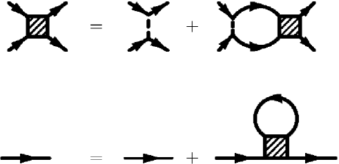
Figure 3: Coupled equations for the $T$-matrix (upper line) and the self-energy (lower line). The $T$-matrix is represented by the square, the bare interaction $V$ by a vertical dashed line, the solid lines correspond to single-particle Green’s functions.

For the same reason, the time-structure of the propagator product in the kernel of Eq. (31) is that of a single two-particle propagator ${\bm{G}}(12)~{}{\bm{G}}(23)={\bm{G}_{2}}(12;34)$. The retarded/advanced components of the $T$-matrix are obtained by applying the Langreth-Wilkins rule (16) to Eq. (31). The Fourier transform of the resulting equation is

$${T}^{R/A}(\bm{p},\bm{p}^{\prime};P)={V}(\bm{p},\bm{p}^{\prime})+\int\!\!\frac{d\bm{p}^{\prime\prime}}{(2\pi)^{3}}~{}V(\bm{p},\bm{p}^{\prime\prime})G_{2}^{R/A}(\bm{p}^{\prime\prime};P)T^{R/A}(\bm{p}^{\prime\prime},\bm{p}^{\prime};P),$$ (32)

with the two-particle propagator

$$G_{2}^{R/A}(\bm{p};P) = \int\!\!\frac{d^{4}P^{\prime}}{(2\pi)^{4}}\int\!\!\frac{d\omega}{(2\pi)}\left[G^{>}(p_{+})G^{>}(p_{-})-G^{<}(p_{+})G^{<}(p_{-})\right]\frac{\delta(\bm{P}-\bm{P}^{\prime})}{\Omega-\Omega^{\prime}\pm i\eta},$$ (33)

where $p_{\pm}={P}/{2}\pm p$ and the four-vector $P=(\bm{P},\Omega)$ is the center of mass four-momentum. The remaining components of the $T$-matrix are given by the relations

$$T^{>,<}(\bm{p},\bm{p}^{\prime};P)=i\int\frac{d^{4}p_{2}}{(2\pi)^{4}}\frac{d^{4}p_{3}}{(2\pi)^{4}}T^{R}(\bm{p},\frac{\bm{p}_{2}-\bm{p}_{3}}{2};P)G^{>,<}(p_{2})G^{>,<}(p_{3})T^{A}(\frac{\bm{p}_{2}-\bm{p}_{3}}{2},\bm{p}^{\prime};P),$$ (34)

which can be interpreted as a variant of the optical theorem. Indeed due to the property $T^{A}=[T^{R}]^{*}$ the product $T^{A}T^{R}=|T|^{2}$ on the r. h. side of Eq. (34) (we use operator notations for simplicity). At the same time $T^{>}-T^{<}=2i\mathop{\rm Im}T^{R}$ [see Eqs. (12) and (13)] which implies that $\mathop{\rm Im}T^{R}\propto G_{2}|T|^{2}$, where $G_{2}$ is defined by Eq. (33). Thus computing $T^{>}-T^{<}$ and comparing the result to Eq. (34) we arrive at another form of the optical theorem

$$(2i)^{-1}T^{<}(\bm{p},\bm{p}^{\prime};P) = f(\omega)f(\omega^{\prime})[1-f(\omega)-f(\omega^{\prime})]^{-1}\mathop{\rm Im}T(\bm{p},\bm{p}^{\prime};P)$$ (35)

$$= g_{B}(\omega+\omega^{\prime})\mathop{\rm Im}T(\bm{p},\bm{p}^{\prime};P),$$

where the second relation follows in equilibrium limit with $g_{B}(\omega)=[1-{\rm exp}(\beta\omega)]^{-1}$ being the Bose distribution function. The contour ordered self-energy in the $T$-matrix approximation is defined as (Fig. 3, second line)

$${\bm{\Sigma}}(1,2)=i\int_{C}d3d4~{}{\bm{T}}(12;34){\bm{G}}(43^{+}).$$ (36)

Since the time dependence of the $T$-matrix is constrained by the time-locality of the interaction, we can immediately write-down the two components

$$i\Sigma^{>,<}(p) = \int\frac{d^{4}p^{\prime}}{(2\pi)^{4}}T^{>,<}\left(\frac{\bm{p}-\bm{p}^{\prime}}{2},\frac{\bm{p}-\bm{p}^{\prime}}{2};p+p^{\prime}\right)_{A}G^{<,>}(p^{\prime}).$$ (37)

where the index $A$ stands for the anti-symmetrization of final states. Explicit expressions for the retarded and advanced components of the self-energy can be obtained, e.g., from the relation $\Sigma^{>}-\Sigma^{<}=2i\mathop{\rm Im}\Sigma^{R}$ and the Kramers-Kronig relation between the real and imaginary parts of the self-energies [7]. Alternatively we can use the Langreth-Wilkins rules to obtain (in operator form)

$$i\Sigma^{R,A}=T^{R,A}G^{<}+T^{<}G^{A,R}.$$ (38)

When the self-energies (37) are substituted in the kinetic equation (29) one finds the Boltzmann transport equation where the collision integrals are evaluated in the $T$-matrix approximation [5, 26, 29]. The on shell scattering $T$-matrix can be directly expressed through the differential scattering cross-section

$$\frac{d\sigma}{d\Omega}(p,P)=\frac{m^{*2}}{(4\pi\hbar^{2})^{2}}|T(p,P)_{A}|^{2},$$ (39)

where $m^{*}$ is the effective mass of the particle. Thus, in the dilute limit and at not too high energies the collision integrals can be evaluated in a model independent way in terms of experimental elastic scattering cross-sections. In dense, correlated systems one needs to take into account the modifications of the scattering by the environment, in this case the drift and collision terms are coupled through the self-energies.

Consider now the equilibrium limit. In this limit the fermionic distribution function reduces to the Fermi-Dirac form. The number of unknown correlations functions is reduced from two to one because one of the equations (20) is redundant. For a complete description of the system the coupled equations for the $T$-matrix and self-energy need to be solved. These are given by Eq. (32) where the retarded two-particle Green’s function is now defined as

$$G_{2}^{R}(\bm{p};P) = \int\!\!\frac{d^{4}P^{\prime}}{(2\pi)^{4}}\int\!\!\frac{d\omega}{(2\pi)}a(p_{+})a(p_{-})Q_{2}(p_{+},p_{-})\frac{\delta(\bm{P}-\bm{P}^{\prime})}{\Omega-\Omega^{\prime}+i\eta},$$ (40)

where $Q_{2}(p_{+},p_{-})=\left[1-f_{F}(p_{+})-f_{F}(p_{-})\right]$ is the Pauli-blocking function. The retarded self-energy is given by the equilibrium limit of Eq. (38) which, upon using the optical theorem (35), becomes

$$\Sigma^{R}(p) = \int\frac{d^{4}p^{\prime}}{(2\pi)^{4}}\Biggl{[}T^{R}(\frac{\bm{p}-\bm{p}^{\prime}}{2},\frac{\bm{p}-\bm{p}^{\prime}}{2};p+p^{\prime})a(p^{\prime})f(\omega^{\prime})$$ (41)

$$\hskip 85.35826pt+2g(\omega+\omega^{\prime})\mathop{\rm Im}T^{R}(\frac{\bm{p}-\bm{p}^{\prime}}{2},\frac{\bm{p}-\bm{p}^{\prime}}{2};p+p^{\prime})\int\frac{d\bar{\omega}}{2\pi}\frac{a(\bm{p}^{\prime},\bar{\omega})}{\omega^{\prime}-\bar{\omega}}\Biggr{]}.$$

Eqs. (32), (40) and (41) form a closed set of coupled integral equations. If the interaction between the fermions is known these equations can be solved numerically by iteration. In the context of nuclear physics this scheme is known also as the Self-Consistent Green’s Functions (SCGF) method [5, 32, 33, 34, 35, 36, 37, 38, 39, 40, 41, 42, 43, 44, 45, 46]. Once the single particle Green’s function (or equivalently the self-energy) is determined, the free energy of the system can be computed from the thermodynamic relation

$$F=E-\beta^{-1}S,$$ (42)

where the internal energy is

$$E=g\int\frac{d^{4}p}{(2\pi)^{4}}\frac{1}{2}\left[\omega+\epsilon(p)\right]a(p)f_{F}(\omega),$$ (43)

and the entropy $S$ is given by the combinatorial formula

$$S=g\int\frac{d^{4}p}{(2\pi)^{4}}a(p)\left\{f_{F}(\omega){\rm ln}f_{F}(\omega)+[1-f_{F}(\omega)]{\rm ln}[1-f_{F}(\omega)]\right\}.$$ (44)

Here $g$ is the spin-isospin degeneracy factor; $g=2$ for (unpolarized) neutron matter and $g=4$ for isospin symmetric nuclear matter. An important feature of the $T$-matrix theory is that it preserves the particle hole-symmetry which, as we have seen, is fundamental for the conservation laws to hold. These can be verified by integrating Eq. (29) with appropriate weights to recover the flow equations for the energy and momentum. Another attractive feature of this theory is that its low-density (high-temperature) limit is the free-space scattering theory. The latter can be constrained by experiments. The structure of the theory and the numerical effort needed for its solution is simplified in this limit, since instead of working with the full spectral function (21) one can approximate it with the $\gamma(p)=0$ limit, i.e. a $\delta$-function. Another interesting limit is that of low temperatures. If the damping is dropped, but the renormalization of the on-shell self-energies is retained (i.e. the real part of the self-energy is expanded with respect to small deviations from the Fermi-momentum $p_{F}$) the spectral function reduces to

$$a(p)=2\pi Z(\bm{p})\delta(\omega-\xi(\bm{p})),\quad\quad\xi(p)=p_{F}(p-p_{F})/m^{*}-\mu^{*},$$ (45)

where $\mu^{*}\equiv-\epsilon(p_{F})+\mu-\mathop{\rm Re}\Sigma(p_{F})$ is the effective chemical potential; the effective mass and the wave function renormalization are defined as

$$\frac{m^{*}}{m}=\left(1+\frac{m}{p_{F}}\partial_{p}\mathop{\rm Re}\Sigma(p)|_{p=p_{F}}\right)^{-1},\quad\quad Z(\bm{p})=\left(1-\partial_{\omega}\mathop{\rm Re}\Sigma(\omega,p_{F})|_{\omega=\xi}\right)^{-1}.$$ (46)

With these approximations one recovers the elementary excitations of the Landau Fermi-liquid theory - the dressed quasiparticles. Retaining the quasiparticle damping, i.e. using the small $\gamma(p)$ approximation, Eq. (23), leads to virial corrections to the quasiparticle pictures. We shall discuss these corrections in more detail in Subsec. 2.2.4.

The $T$-matrix approximation to self-energy leads to a model which satisfies the conservation laws (it is said that the model is conserving). In addition to being conserving any model that is based on an certain approximation to the self-energy needs to be thermodynamically consistent. The thermodynamic consistency refers to the fact that thermodynamic quantities like free energy or pressure computed from different expressions agree. An example is the Hugenholtz-van Hove theorem [47], which relates the single particle energy at the Fermi-surface to the binding energy $E_{B}$ at the zero temperature

$$\varepsilon(p_{F})=\frac{P}{\rho}+E_{B},$$ (47)

where the pressure is defined as $P=\rho^{2}\partial_{\rho}E_{B}$. Another example is the equivalence of the thermodynamic pressure defined above and the virial pressure, the latter being the pressure calculated from the energy momentum tensor.

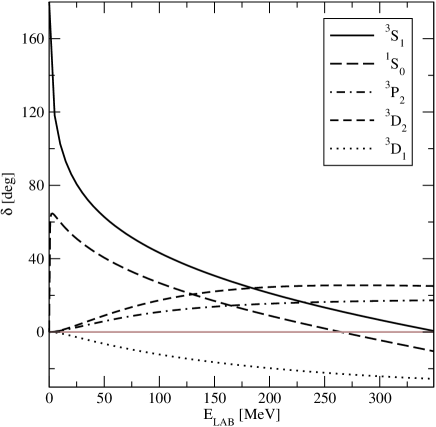
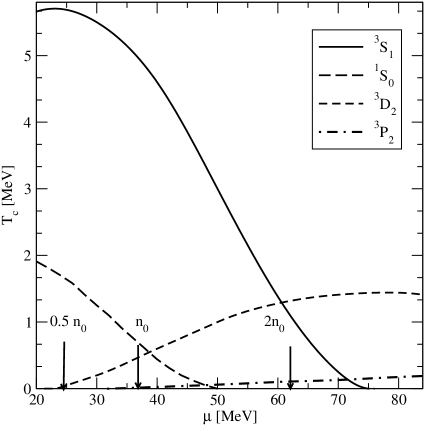
Figure 4: Left panel. Dependence of the experimental scattering phase shifts in the ${}^{3}S_{1}$, ${}^{3}P_{2}$, ${}^{3}D_{2}$, and ${}^{3}D_{1}$ partial waves on the laboratory energy. Right panel. The dependence of the critical temperatures of superfluid phase transitions in the attractive channels on the chemical potential. The corresponding densities are indicated by arrows. The critical temperatures $T_{c}$ are computed from the $T$-matrix instability [49].

2.2.1 Pairing instability and precursor phenomena

We have seen that in the low-density and high-temperature domain the $T$-matrix theory is well defined in terms of free-space parameters and it can be used at arbitrary temperatures and densities. In the opposite limit of high densities and low temperatures its validity domain is restricted to the temperatures above the critical temperature $T_{c}$ of superfluid phase transition. The physical reason is that at $T_{c}$ there appears a bound state in the particle-particle channel - the Cooper pair. This has far reaching consequences, since the onset of macroscopic coherence implies that the average value of correlation function $\langle\psi(x)\psi(x)\rangle\neq 0$, which requires a doubling of the number of Green’s function needed to describe the superfluid state. At temperatures $T\geq T_{c}$ the $T$-matrix is strongly enhanced for particle scattering with equal and opposite momenta and it diverges at $T=T_{c}$.

Partial wave analysis of the nucleon-nucleon scattering allows us to identify the attractive channels (which feature positive phase shifts). The critical temperature in each channel is determined from the condition that the $T$-matrix, Eq. (32), develops a pole for parameter values $\tilde{P}=(\Omega,\bm{P})=(2\mu,0)$ [7, 28, 48, 49, 50]. To illustrate this feature assume a rank-one separable interaction $V(\bm{p},\bm{p}^{\prime})=\chi(\bm{p})\chi(\bm{p}^{\prime})$ and the quasiparticle approximation. The solution of Eq. (32), which parametrically depends on the chemical potential and the temperature is

$$T(\bm{p},\bm{p}^{\prime},\tilde{P})=V(\bm{p},\bm{p}^{\prime})\left[1-\int\frac{d^{3}p}{(2\pi)^{3}}\chi^{2}(\bm{p})G_{2}(\bm{p},\tilde{P})\right]^{-1}.$$ (48)

At the critical temperature both the real and imaginary parts of the expression in braces vanish; the zero of the real part determines the critical temperature $T_{c}$. Fig. 4 shows the neutron-proton scattering phase shifts which are relevant for the pairing pattern in the isospin symmetric nuclear matter (left panel) and the associated critical temperatures (right panel) determined from the $T$-matrix instability [49]. For isospin symmetric systems the most attractive channels are the tensor channel ${}^{3}S_{1}-^{3}D_{1}$ and the ${}^{3}D_{2}$ channel where only the neutrons and protons interact. For small isospin asymmetries, which correspond to $\alpha=(\rho_{n}-\rho_{p})/(\rho_{n}+\rho_{p})\leq\alpha_{c}\simeq 0.1$, where $\rho_{n}$ and $\rho_{p}$ are the neutron and proton densities, the mismatch in the Fermi-surfaces of neutrons and protons suppresses the pairing [50, 51, 52, 53, 54, 55, 56, 57, 58, 59].

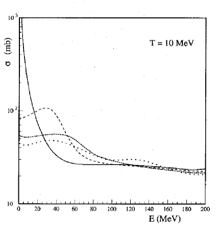
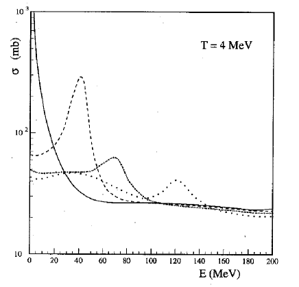
Figure 5: The cross section in neutron matter as a function of relative energy of particles ($E=E_{\rm LAB}/2$) for temperatures $T=10$ MeV (left panel) and $T=4$ MeV (right panel) and densities $\rho=0$ (solid line), $\rho=\rho_{0}/5$ (dashed line), $\rho=\rho_{0}/2$ (dashed-dotted line) and $\rho=\rho_{0}$ dotted line.

For large asymmetries typical for compact stars the pairing is among same isospin particles in the ${}^{1}S_{0}$ and ${}^{3}P_{2}$ channels. Because of the smallness of the charge symmetry breaking effects, the critical temperatures in the ${}^{1}S_{0}$ and ${}^{3}P_{2}$ shown in Fig. 4 channels are representative for neutron star matter as well (note however that the relation between the density and the chemical potential changes) [60, 61]. Some models of neutron star matter which predict kaon condensation at high densities feature isospin symmetric nucleonic matter, in which case the high-density $D$-wave neutron-proton paring will dominate the $P$-wave neutron-neutron pairing [50]. The scattering characteristics of the system such as the phase-shifts and the scattering cross-sections are affected by the pairing instability, since these are directly related to the on-shell $T$-matrix. The phase-shifts in a pairing channel change by $\pi/2$ at the critical temperature when the energy equals $2\mu$. According to the Levinson theorem, this corresponds to the appearance of bound state (Cooper pair). For many practical applications the cross-section is the relevant quantity. According to Eq. (39) the cross-section being proportional to the $T$-matrix will diverge at $T_{c}$ [28, 49, 62, 63, 64, 65, 66]. The precursor effect of the superfluid phase transition on the neutron-neutron scattering cross-section in the low temperature neutron matter is shown in Fig 5 [62]. The cross-section develops a spike for lower temperature as a precursor of the onset of superfluid in neutron matter in the ${}^{1}S_{0}$ interaction channel. The largest enhancement is seen for the density $\rho=0.5\rho_{0}$ which is closest to the maximum of the critical temperature as a function of density. The above precritical behavior of the cross-section has a significant effect on the transport and radiation processes in matter, for example, it could lead to a critical opalescence in the transport phenomena.

2.2.2 $T$-matrix theory in the superfluid phase

We have seen in the previous section that at the critical temperature of superfluid phase transition the two-body scattering $T$-matrix develops a singularity, which is related to the instability of the normal state with respect to formation of Cooper pairs; this is manifested in pole of the two-body $T$-matrix when the relative energy of interacting fermions is twice their chemical potential. Thus, the $T$-matrix theory described above breaks down at the temperature $T=T_{c}$. A $T$-matrix theory appropriate for temperatures below $T_{c}$ can be formulated in terms of the normal and anomalous Green’s functions [7]. To account for pair correlation we represent each Green’s function in the Keldysh-Schwinger formalism as a $2\times 2$ matrix in the Gor’kov space:

$${\bm{G}\!\!\!\!G}(x,x^{\prime})=\left(\begin{array}[]{cc}{\bm{G}}_{\alpha\beta}(x,x^{\prime})&{\bm{F}}_{\alpha\beta}(x,x^{\prime})\\ -{\bm{F}}^{\dagger}_{\alpha\beta}(x,x^{\prime})&\tilde{\bm{G}}_{\alpha\beta}(x,x^{\prime})\\ \end{array}\right)=\left(\begin{array}[]{cc}-i\langle T\psi_{\alpha}(x)\psi_{\beta}^{\dagger}(x^{\prime})\rangle&\langle\psi_{\alpha}(x)\psi_{\beta}(x^{\prime})\rangle\\ \langle\psi_{\alpha}^{\dagger}(x)\psi_{\beta}^{\dagger}(x^{\prime})\rangle&-i\langle\tilde{T}\psi_{\alpha}(x)\psi_{\beta}^{\dagger}(x^{\prime})\rangle\\ \end{array}\right),$$ (49)

where ${\bm{G}}_{\alpha\beta}(x,x^{\prime})$ and ${\bm{F}}^{\dagger}_{\alpha\beta}(x,x^{\prime})$ are referred to as the normal and anomalous propagators. The $4\times 4$ matrix Green’s function satisfies the familiar Dyson equation

$${\bm{G}\!\!\!\!G}_{\alpha\beta}(x,x^{\prime})={\bm{G}\!\!\!\!G}^{0}_{\alpha\beta}(x,x^{\prime})+\sum_{\gamma,\delta}\int\!\!d^{4}x^{\prime\prime}d^{4}x^{\prime\prime\prime}{\bm{G}\!\!\!\!G}^{0}_{\alpha\gamma}(x,x^{\prime\prime\prime}){\bm{\Sigma}\!\!\!\!\,\Sigma}_{\gamma\delta}(x^{\prime\prime\prime},x^{\prime\prime}){\bm{G}\!\!\!\!G}_{\delta\beta}(x^{\prime\prime},x^{\prime}),$$ (50)

where the free propagators ${\bm{G}\!\!\!\!G}^{0}_{\alpha\beta}(x,x^{\prime})$ are diagonal in the Gor’kov space. We consider below uniform fermionic systems; the propagators now depend only on the difference of their arguments due to translational symmetry. A Fourier transformation of Eq. (50) with respect to the difference of the space arguments of the two-point correlation functions leads to on- and off-diagonal Dyson equations

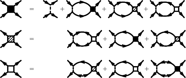
Figure 6: The ladder series in a superfluid fermionic system. The dashed lines correspond to the driving interaction, single arrow lines to normal propagators and double arrow lines to anomalous propagators. The filled square is the counterpart of the unpaired state $T$-matrix, the shaded and empty squares are specific to superfluid state.

$${\bm{G}}_{\alpha\beta}(p) = {\bm{G}}_{0\alpha\beta}(p)+{\bm{G}}_{0\alpha\gamma}(p)\left[{\bm{\Sigma}}_{\gamma\delta}(p){\bm{G}}_{\delta\beta}(p)+{\bm{\Delta}}_{\gamma\delta}(p){\bm{F}}d_{\delta\beta}(p)\right],$$ (51)

$${\bm{F^{\dagger}}}_{\alpha\beta}(p) = {\bm{G}}_{0\alpha\gamma}(-p)\left[{\bm{\Delta}}^{\dagger}_{\gamma\delta}(p){\bm{G}}_{\delta\beta}(p)+{\bm{\Sigma}}_{\gamma\delta}(-p){\bm{F}}{\bm{\Delta}}_{\delta\beta}(p)\right],$$ (52)

where $p$ is the four-momentum, ${\bm{G}}_{0\alpha\beta}(p)$ is the free normal propagator, and ${\bm{\Sigma}}_{\alpha\beta}(p)$ and ${\bm{\Delta}}_{\alpha\beta}(p)$ are the normal and anomalous self-energies. Summation over repeated indices is understood. Specifying the self-energies in terms of the propagators closes the set of equations consisting of (51) and (52) and their time-reversed counterparts [$\tilde{\bm{G}}_{\alpha\beta}(p)$ and ${\bm{F}}_{\alpha\beta}(p)$]. The particle-particle scattering in the superfluid state is described by three topologically different vertices shown in Fig. 6 [67]. We write out the explicit expression for the retarded components of the $T$-matrix in operator form [their form in the momentum space in identical to Eq. (32)]

$$T^{(1)} = V\left[1+S_{GG}T^{(1)}+S_{FG}T^{(2)}+S_{FF}T^{(3)}\right],$$ (53)

$$T^{(2)} = V\left[S_{FF}T^{(3)}+S_{GG}T^{(1)}+S_{FG}T^{(2)}\right],$$ (54)

$$T^{(3)} = V\left[S_{FG}T^{(2)}+S_{GG}T^{(3)}+S_{FF}T^{(1)}\right],$$ (55)

where the two-particle retarded propagators are defined as

$$S_{GG}=G^{>}G^{>}-G^{<}G^{<},\quad S_{GF}=G^{>}F^{>}-F^{<}G^{<},\quad S_{GF}=F^{>}F^{>}-F^{<}F^{<},$$ (56)

and their structure in the momentum space is given by Eq. (33). To close the system of equations we define the normal and anomalous self-energies for the off-diagonal elements of the Schwinger-Keldysh structure

$$i\Sigma^{>,<} = T^{(1)>,<}G^{<,>}+T^{(2)>,<}F^{<,>},$$ (57)

$$i\Delta^{>,<} = T^{(3)>,<}F^{<,>}+T^{(2)>,<}G^{<,>},$$ (58)

which are shown in Fig. 7.

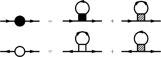
Figure 7: The normal (filled circle) and anomalous (empty circle) self-energies in the superfluid $T$-matrix theory. The self-energies couple through the $T$ matrices appearing in Fig. 6.

The retarded components of the self-energies which solve Dyson equations (51) and (52) can be constructed from Eqs. (57) and (58) via the dispersion relations, e.g.,

$$\Delta^{R}(\omega)=\int_{-\infty}^{\infty}\frac{d\omega^{\prime}}{2\pi}\frac{\Delta^{>}(\omega^{\prime})-\Delta^{<}(\omega^{\prime})}{\omega-\omega^{\prime}+i\eta},$$ (59)

with an analogous relation for $\Sigma^{R}(\omega)$. The system of Eqs. (53)-(55) can be used to derive the collective excitations of the superfluid nuclear matter in particle-particle channel. In the mean field approximation the self-energies decouple from the $T$-matrix equations (53)-(55) and the secular equation determining the frequencies of collective modes for vanishing center-of-mass momentum is

$$\left[A+(4\Delta^{2}-\omega^{2})B\right]\left[A-(4\Delta^{2}A+\omega^{2})B+2\Delta^{2}\omega^{2}B^{2}\right]=0,$$ (60)

where, assuming that the pairing interaction can be approximated by a constant and the integrals regularized by a cut-off, one finds

$$B(\omega)=\lambda\int_{\Delta}^{\infty}\frac{1-2f_{F}(\varepsilon)}{\sqrt{\varepsilon^{2}-\Delta^{2}}}\frac{d\varepsilon}{\omega^{2}-4\varepsilon^{2}+i\omega\eta},\quad A=1+\lambda\int_{\Delta}^{\Lambda}\frac{d\varepsilon}{\sqrt{\varepsilon^{2}-\Delta^{2}}}[1-2f_{F}(\varepsilon)],$$ (61)

where $\lambda$ is an effective coupling constant, $\Lambda$ is an ultraviolet cut-off. The second equation is the stationary gap equation, i.e. $A=0$; the secular equation then leads to the solutions $B(\omega)=0$, $B(\omega)=(2\Delta^{2})^{-1}$, $\omega^{2}=0$ and $\omega=\pm 2\Delta$. Among the first two non-trivial conditions the second one does not have a solution for weakly coupled systems $\lambda\ll 1$ and the collective modes are determined by the secular equation $B(\omega)=0$, whereby the real part of the solution determines the eigenmodes and the imaginary part their damping.

2.2.3 Three-body $T$-matrix and bound states

Up to now we were concerned with the correlations described by the two-body $T$-matrix. The properties of dilute fermions or cold Fermi-liquids (the latter are characterized by a filled Fermi-sea) are well described in terms of two-body correlations between particles or quasi-particle excitations. However, the three-body correlations, which are next in the hierarchy, are important under certain circumstances. We turn now to the three-body problem in Fermi-systems within the formalism developed in the previous sections. As is well known, the non-relativistic three-body problem admits exact free space solutions both for contact and finite range potentials [68, 69]. Skorniakov–Ter-Martirosian–Faddeev equations sum-up the perturbation series to all orders with a driving term corresponding to the two-body scattering $T$-matrix embedded in the Hilbert space of three-body states. The counterparts of these equations in the many-body theory were first formulated by Bethe [70] to access the three-hole-line contributions to the nucleon self-energy and the binding of nuclear matter (Bethe’s approach is discussed in Subsection 2.3). More recently, alternative forms of the three-body equations in a background medium have been developed that use either an alternative driving force (the particle-hole interaction or scattering $T$-matrix) [29, 71, 72, 73] or/and adopt an alternative version of the free-space three-body equations, known as the Alt-Grassberger-Sandhas form [74, 75, 76].

The resummation series for three-body scattering amplitudes can be written down in terms of the three-body interaction ${\cal V}$ as [29]

$${\cal T}={\cal V}+{\cal V}\,{\cal G}\,{\cal V}={\cal V}+{{\cal V}}\,{{\cal G}}_{0}\,{{\cal T}},$$ (62)

where ${\cal G}_{0}$ and ${\cal G}$ are the free and full three-particle Green’s functions (we use the operator form for notational simplicity; each operator, as in the two-particle case, is ordered on the contour). If the three-body forces that act simultaneously between the three-particle are neglected, the interaction in Eq. (62) is simply the sum of pairwise interactions: ${{\cal V}}={{\cal V}}_{12}+{{\cal V}}_{23}+{{\cal V}}_{13}$, where ${{\cal V}}_{\alpha\beta}$ is the interaction potential between particles $\alpha$ and $\beta$. The kernel of Eq. (62) is not square integrable: the potentials ${{\cal V}}_{\alpha\beta}$ introduce delta-functions due to momentum conservation for the spectator non-interacting particle and the iteration series contain singular terms (e.g., of type ${{\cal V}}_{\alpha\beta}{{\cal G}}_{0}{{\cal V}}_{\alpha\beta}$ to the lowest order in the interaction).

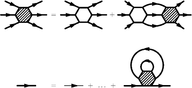
Figure 8: Coupled integral equations for the three-body ${\cal T}$-matrix (first line) and the single particle propagator (second line). The shaded vertex stands for the amplitude $T^{(i)}$, the empty vertex stands for a channel $T_{kj}$ matrix. The second line shows the Dyson equation for the single particle Green’s function including the contribution from three-body scattering. The dots stand for the contribution from the two-body scattering shown in Fig 3.

The problem is resolved by summing up the ladder series in a particular channel (specified by the indices $\alpha,\beta$) to all orders [69]. This summation defines the channel ${{\cal T}}_{\alpha\beta}$-matrix, which is essentially the two-body $T$-matrix embedded in the Hilbert space of three-particles states

$${{\cal T}}_{\alpha\beta}={{\cal V}}_{\alpha\beta}+{{\cal V}}_{\alpha\beta}\,{{\cal G}}_{0}\,{{\cal T}}_{\alpha\beta}.$$ (63)

The three-body ${\cal T}$-matrix can be decomposed as ${{\cal T}}={{\cal T}}^{(1)}+{{\cal T}}^{(2)}+{{\cal T}}^{(3)},$ where

$${{\cal T}}^{(\alpha)} = {{\cal V}}_{\beta\gamma}+{{\cal V}}_{\beta\gamma}\,{{\cal G}}_{0}\,{{\cal T}},$$ (64)

and $\alpha\beta\gamma=123,\,231,\,312$. Now, Eqs. (63) and (64) are combined to eliminate the interaction terms ${\cal V}_{\alpha\beta}$ and one is left with three coupled integral equations for ${{\cal T}}^{(\alpha)}$ ($\alpha=1,2,3$)

$${{\cal T}}^{(\alpha)}={{\cal T}}_{\beta\gamma}+{{\cal T}}_{\beta\gamma}\,{{\cal G}}_{0}\,\left({{\cal T}}^{(\beta)}+{{\cal T}}^{(\gamma)}\right),$$ (65)

where the driving terms are the channel $T$-matrices. The new equations are non-singular Fredholm type-II integral equations. Note that their formal structure is identical to the Faddeev equations in the vacuum [69], however their physical meaning is different. To see the physical content of Eqs. (65) we need to convert the contour ordered equations into equations for the components (so that the KB ansatz (20) can be applied) and to transform them from the operator form into momentum representation. Proceeding as in Subsection 2.1, the retarded component of Eq. (64) reads

$${\cal T}^{R\,(1)}(t,t^{\prime})=\ {\cal T}^{R}_{23}(t,t^{\prime})+\int\left[\ {\cal T}^{R\,(2)}(t,\bar{t})+{\cal T}^{R\,(3)}(t,\bar{t})\right]{\cal G}_{0}^{R}(\bar{t},t^{\prime\prime}){\cal T}^{R}_{23}(t^{\prime\prime},t^{\prime})d\bar{t}dt^{\prime\prime},$$ (66)

were we used the time-locality of the interaction and omitted the momentum arguments of the functions (for the explicit expressions see ref. [29]). Next, to apply the KB ansatz we need to specify the particle hole content of the three-body $T$-matrix, i. e. assign each incoming/outgoing state a particle or a hole. Figure 8 shows the Feynman diagram for the three-body $T$-matrix where all the incoming (outgoing) states are particles (holes). The remaining three-body $T$-matrices are obtained by reverting the direction of the arrows in the diagram. Depending on the particle-hole content of the three-body $\cal T$-matrix (in the sense above) the intermediate state retarded Green’s function is

$${\cal G}_{0}^{R}(t_{1},t_{2}) = \theta(t_{1}-t_{2})\left\{\begin{array}[]{cl}G^{>}G^{>}G^{>}(t_{1},t_{2})-(>\,\leftrightarrow\,<)&~{}(3p)\\ G^{>}G^{>}G^{<}(t_{1},t_{2})-(>\,\leftrightarrow\,<)&~{}(2ph)\\ G^{>}G^{<}G^{<}(t_{1},t_{2})-(>\,\leftrightarrow\,<)&~{}(p2h)\\ G^{<}G^{<}G^{<}(t_{1},t_{2})-(>\,\leftrightarrow\,<)&~{}(3h)\\ \end{array}\right.$$ (71)

where $p$ and $h$ refer to particle and hole states, the brackets [e. g. (2ph)] indicate the particle-hole content of Green’s function; for simplicity the time argument in a product is shown only once. The short hand $>\,\leftrightarrow\,<$ stands for a term where all the $G^{<}$ and $G^{>}$ functions are interchanged. Upon applying the KB ansatz and Fourier transforming Eq. (66) one finds

$${\cal T}^{R\,(1)}(\Omega)=\ {\cal T}^{R}_{23}(\Omega^{\prime})+\int\left[\ {\cal T}^{R\,(2)}(\Omega^{\prime})+{\cal T}^{R\,(3)}(\Omega^{\prime})\right]\frac{Q_{3}(\Omega^{\prime})}{\Omega-\Omega^{\prime}+i\eta}{\cal T}^{R}_{23}(\Omega^{\prime})d\Omega^{\prime},$$ (72)

where the the four-momentum space is spanned in terms of Jacobi coordinates, $K=p_{\alpha}+p_{\beta}+p_{\gamma},\quad k_{\alpha\beta}=(p_{\alpha}-p_{\beta})/2,\quad q_{\gamma}=(p_{\alpha}+p_{\beta})/3-2p_{\gamma}/3,$ the center-of-mass energy $\Omega\equiv K_{0}$ and

$$Q_{3}(p_{\alpha},p_{\beta},p_{\gamma})=a(p_{\alpha})a(p_{\beta})a(p_{\gamma})\left\{[1-f_{F}(p_{\alpha})][1-f_{F}(p_{\beta})][1-f_{F}(p_{\gamma})]-f_{F}(p_{\alpha})f_{F}(p_{\beta})f_{F}(p_{\gamma})\right\}.$$ (73)

This form of three-body equation incorporates off-mass-shell propagation if the spectral function is taken in the form (21). The quasiparticle (on-mass-shell propagation) limit follows by using (45) in Eq. (73). Thus, the many-body environment modifies the three-body equation in a twofold way: first, the single-particle spectrum is renormalized in the resolvent of Eq. (72) [which becomes explicit after taking the quasiparticle limit], second, the intermediate state propagation is statistically occupied according to Eq. (73). The limit $Q\to 1$ and $a(\omega)=2\pi\delta(\omega-\epsilon(\bm{p}))$ recovers the original Faddeev equations.

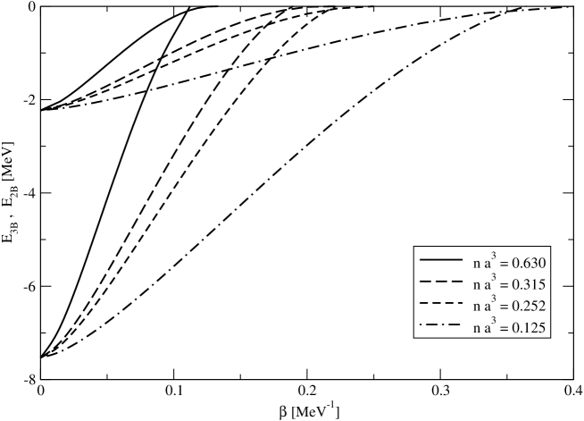
Figure 9: Dependence of the three-body and two-body bound state energies on the inverse temperature for fixed parameter values $na^{3}$, where $n$ is the density and $a$ the neutron-proton triplet scattering length.

The single-particle self-energy obtains contributions from the three-body $T$-matrix, which is shown in Fig. 8. In the case of $(3p)$ scattering $T$-matrix the three-body self-energy is written as

$${\mathfrak{S}}^{>,<}(p_{1})=\int_{p_{2}p_{3}}\Bigl{[}{\cal T}^{(1)}_{>,<}(\bm{k}_{23},\bm{q}_{1},K)+{\cal T}^{(2)}_{>,<}(\bm{k}_{13},\bm{q}_{2},K)+{\cal T}^{(3)}_{>,<}(\bm{k}_{12},\bm{q}_{3},K)\Bigr{]}G^{>}(p_{2})\,G^{>}(p_{3}),$$ (74)

where we use the notation $\int_{p}=d^{4}p/(2\pi)^{4}$. The optical theorem relates the $T^{>,<}$ components of the three-body $T$-matrix to the retarded component given by Eq. (72):

$${\cal T}^{<}(\bm{k}_{23},\bm{q}_{1},\bm{k}_{23}^{\prime},\bm{q}_{1}^{\prime};K)=\sum_{\alpha,\beta}\int_{p_{4},p_{5},p_{6}}{\cal T}^{(\alpha)\,R}(\bm{k}_{23},\bm{q}_{1},\bm{k}_{45},\bm{q}_{6};K)G^{<}(p_{4})\,G^{<}(p_{5})\,G^{<}(p_{6})$$

$$\hskip 56.9055pt\times{\cal T}^{(\beta)\,A}(\bm{k}_{45},\bm{q}_{6},\bm{k}_{23}^{\prime},\bm{q}_{1}^{\prime};K)(2\pi)^{4}\,\delta^{4}(K-p_{4}-p_{5}-p_{6}).$$ (75)

To illustrate the usefulness of the three-body equations discussed above we show in Figure 9 the binding energy of a three-body bound state (triton) in nuclear matter as a function of the inverse temperature for several values of density, $n$, measured in units of $a^{-3}$, where $a=5.4$ fm is the neutron-proton triplet scattering length. The asymptotic free-space value of the binding energy in this model is $E_{3B}=7.53$ MeV. The binding energy was obtained from the solution of the homogeneous counterpart of Eq. (72) in quasiparticle limit assuming free single particle spectrum [77]. In addition we show the temperature dependence of the deuteron energy $E_{2B}(\beta)$ obtained within the same approximations from the homogeneous counterpart of Eq. (32). The continuum for the break-up process $3B\to 2B+N$, where $N$ refers to nucleon, is temperature/density dependent as well and is found from the condition $E_{3B}(\beta)=E_{2B}(\beta)$.

2.2.4 The quantum virial equation of state

The equation of the state of a Fermi-system characterized by small damping (long-lived, but finite life-time quasiparticles) can be written in the form of a virial expansion for density [27, 28, 29]

$$n(\beta,\mu)=\int\frac{d^{4}p}{(2\pi)^{4}}\left[a(E,\bm{p})f_{F}(E)+b(E,\bm{p})g_{B}(E)+c(E,\bm{p})f_{F}(E)\right],$$ (76)

where the virial coefficients $a(p)$, $b(p)$, and $c(p)$ are the one-, two- and three-particle spectral functions. Below we show that the virial coefficients $b(E,\bm{p})$ and $c(E,\bm{p})$ can be written entirely in terms of the two- and three-body $T$-matrices and their derivatives. In the dilute limit the on-shell $T$-matrices are related to the scattering phase-shifts; since the damping in this limit is small a direct relation between the scattering observables in free-space and the equation of state can be established. We have seen that in the small damping limit the spectral function can be approximated by Eqs. (23) and (24) to leading order. Thus our starting point is the expression for the density of the system which we write as

$$n(\beta,\mu)=\int\frac{d^{3}p}{(2\pi)^{3}}f_{F}(\varepsilon_{p})+\int\frac{d^{4}p}{(2\pi)^{4}}a(\omega)\left[f_{F}(\omega)-f_{F}(\varepsilon)\right].$$ (77)

The first term is the contribution from the “uncorrelated” quasiparticles (note that the notion of quasiparticle already requires correlations which renormalize the single particle spectrum, however the quasiparticles are still characterized by a sharp relation between the energy and the momentum as the ordinary particles). The second term is the correlated density which, upon using Eqs. (23) and (24), becomes

$$n_{\rm corr}(\beta,\mu)=-\int\!\!\frac{d^{4}p}{(2\pi)^{4}}\gamma(p)\partial_{\omega}\left(\frac{\cal P}{\omega-\varepsilon_{p}}\right)\left[f_{F}(\omega)-f_{F}(\varepsilon_{p})\right].$$ (78)

Let us first evaluate this expression neglecting the three-body correlations. The damping can be written as $\gamma(p)=i[\Sigma^{<}(p)-\Sigma^{>}(p)]=-2\mathop{\rm Im}\Sigma$ where the self-energies are given by Eqs. (37). Using the optical theorem for the two-body $T$-matrix we obtain

$$\gamma(p_{1})=2\int\frac{d^{4}p_{2}}{(2\pi)^{4}}a(\omega_{2})\,\left[g_{B}(\omega_{1}+\omega_{2})+f_{F}(\omega_{2})\right]{\rm Im}T^{R}(\frac{\bm{p}_{1}-\bm{p}_{2}}{2},\frac{\bm{p}_{1}-\bm{p}_{2}}{2};p_{1}+p_{2}),$$ (79)

where the spectral function can be taken in the quasiparticle approximation at the order of interest. Substituting the damping in Eq. (78) and using the identity $\left[g_{B}(E)+f_{F}(\omega_{2})\right]\left[f_{F}(E-\omega_{2})-f_{F}(\omega_{1})\right]=\left[g_{B}(E)-g_{B}(\omega_{1}+\omega_{2})\right]\left[1-f_{F}(\omega_{1})-f_{F}(\omega_{2})\right],$ we recover the second term of the expansion (77) with the second (quantum) virial coefficient [27, 28]

$$b(\varepsilon_{p_{1}},E) = 2\int\frac{d^{3}p_{2}}{(2\pi)^{3}}Q_{2}(\varepsilon_{p_{1}},\varepsilon_{p_{2}})\Bigg{[}{\rm Im}T^{R}(\frac{\bm{p}_{1}-\bm{p}_{2}}{2},\frac{\bm{p}_{1}-\bm{p}_{2}}{2};E)\frac{d}{dE}{\rm Re}{R}^{R}(E)$$ (80)

$$+ {\rm Im}{R}^{R}(E)\,\frac{d}{dE}{\rm Re}T^{R}(\frac{\bm{p}_{1}-\bm{p}_{2}}{2},\frac{\bm{p}_{1}-\bm{p}_{2}}{2};E)\Biggr{]},$$

where ${R}^{R}(E)=\left[E-\varepsilon(p_{1})-\varepsilon(p_{2})+i\eta\right]^{-1}$ is the two-particle resolvent. For systems which support bound states in the free space the second virial coefficient obtains contributions both from the negative energy bound states and the continuum of scattering states. The bound states appear as simple poles of the two-body $T$-matrix on the real axis. The scattering states can be characterized by the phase-shifts in a given partial wave channel, after the two-body scattering $T$-matrix is expanded into partial waves. The phase shift is defined simply as the phase of the on shell complex valued matrix $T_{\alpha}(p,p;E=\varepsilon(p)+\varepsilon(p))=|T_{\alpha}(p,p,E)|{\rm exp}~{}({\delta_{\alpha}})$ where $\alpha=TSJLL^{\prime}$ specifies the partial wave channel in terms of total spin $S$, isospin $T$ and angular $L$ and total $J$ momenta. The second virial coefficient can now be written in terms of the bound state energies $E_{\beta}$ (where $\beta=1,2...$ enumerate the poles of the $T$-matrix) and the scattering phase shifts

$$b(\varepsilon_{p_{1}},E)=2\pi\sum_{\beta}\delta(\omega-E_{\beta})+2\sum_{\alpha}~{}c_{\alpha}~{}2\,{\rm sin}^{2}\delta_{\alpha}(E)\frac{d\delta_{\alpha}(E)}{dE},$$ (81)

where $c_{\alpha}$ are channel dependent constants. In the non-degenerate limit one recovers the classical Beth-Uhlenbeck formula [78].

The third virial coefficient is obtained by including the contribution to the damping from the three-body processes ${\mathfrak{G}}=i({\mathfrak{S}}^{<}-{\mathfrak{S}}^{>})=-2\mathop{\rm Im}{\mathfrak{S}}$, where the self-energies are defined by Eq. (74). Now the correlated density is written as

$$n_{\rm corr}(\beta,\mu)=-\int\!\!\frac{d^{4}p}{(2\pi)^{4}}[\gamma(p)+{\mathfrak{G}}(p)]\partial_{\omega}\left(\frac{\cal P}{\omega-\varepsilon_{p}}\right)\left[f_{F}(\omega)-f_{F}(\varepsilon_{p})\right].$$ (82)

The damping ${\mathfrak{G}}(p)$ is expressed in terms of the ${\cal T^{<,>}}$ matrices which in turn can be related to the retarded component ${\cal T^{R}}$ if we use the optical theorem obeyed by the three-body matrices. The off-shell form of the optical theorem reads

$${\rm Im}{\cal T}^{R}(\bm{k}_{23}\bm{q}_{1},\bm{k}_{45}\bm{q}_{6};K) = \frac{i}{2}\sum_{\alpha\beta}\int_{p_{4},p_{5},p_{6}}{\cal T}^{R\,(\alpha)}(\bm{k}_{23}\bm{q}_{1},\bm{k}_{45}\bm{q}_{6};K)\Bigl{[}G^{<}(p_{4})G^{<}(p_{5})G^{<}(p_{6})$$ (83)

$$-G^{>}(p_{4})G^{>}(p_{5})G^{>}(p_{6})\Bigr{]}{\cal T}^{A\,(\beta)}(\bm{k}_{45}\bm{q}_{6},\bm{k}_{23}\bm{q}_{1};K)\delta^{4}\left(K-p_{4}-p_{5}-p_{6}\right),$$

where the proper momenta $p_{i}$ $(i=1,2,3)$ and Jacobi momenta $k_{ij}$ $q_{k}$ transform into each other according to the rules given after Eq. (72). Since we seek corrections that are first order in damping, the ${\cal T}$-matrix in expression (82) can be taken in the quasiparticle approximation; the on-shell optical theorem implies then

$${\cal T}^{<}(\bm{k}_{23}\bm{q}_{1},\bm{k}_{45}\bm{q}_{6};K) = 2if_{F}\left(\omega_{1}+\omega_{2}+\omega_{3}\right){\rm Im}{\cal T}^{R}(\bm{k}_{23}\bm{q}_{1},\bm{k}_{45}\bm{q}_{6};K),$$ (84)

and an analogous expression for ${\cal T}^{>}$ with the replacement $f_{F}(\omega)\to 1-f_{F}(\omega)$. Evaluating the three-body damping ${\mathfrak{G}}(p)$ with the help of on-shell optical theorem one arrives at the third quantum virial coefficient [29]

$$c(\varepsilon_{p_{1}},E) = 2\int_{{\bm{p}}_{2}{\bm{p}}_{3}}Q_{3}(\varepsilon_{p_{1}},\varepsilon_{p_{2}},\varepsilon_{p_{3}})\Bigl{[}{\rm Im}{\cal T}^{R}(\bm{k}_{23}\bm{q}_{1},\bm{k}_{23}\bm{q}_{1};K)\frac{d}{dE}{\rm Re}{\cal R}(E)$$ (85)

$$+ {\rm Im}{\cal R}(E)\frac{d}{dE}{\rm Re}{\cal T}(\bm{k}_{23}\bm{q}_{1},\bm{k}_{23}\bm{q}_{1};K)\Bigr{]},$$

and where ${\cal R}=\left[E-\varepsilon_{p_{1}}-\varepsilon_{p_{2}}-\varepsilon_{p_{3}}+i\eta\right]^{-1}$is the three-particle resolvent. The third virial coefficient can be decomposed into scattering and bound-state contributions in analogy to the two-body case. Complications arise in attractive systems where apart from the three-body bound states one needs to take into account the break-up, recombination and rearrangement channels which are absent in the two-body case. The knowledge of the virial expansion (76) completely specifies the equation of state of the system; the pressure can be computed from the Gibbs equation

$$p(\mu,\beta)=\int_{-\infty}^{\mu}d\mu^{\prime}n(\mu^{\prime},\beta).$$ (86)

The common form of the equation of state $p(n,\beta)$ is obtained upon eliminating the parametric dependence on the chemical potential $\mu$. The theories based on the second virial coefficients smoothly interpolate between the classical gas theory at low densities and high temperatures and the Bruckner-Bethe-Goldstone theory at low temperatures and high densities [28]. The effects of the third quantum virial coefficient on the equation of state of nuclear matter have not been studied to date.

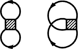
Figure 10: The lowest order diagrams of the BBG theory for the direct (left) and the exchange (right) contributions to the energy. The square denotes the $K$-matrix, the solid lines correspond to the hole propagators.

2.3 The Bruckner-Bethe-Goldstone theory

In a number of cases it is more convenient to evaluate the ground state energy, or at finite temperatures the thermodynamic potential, directly instead of first obtaining the Green’s function from the Dyson equations and then calculating the thermodynamic quantities. The Brueckner-Bethe-Goldstone (BBG) theory evaluates the ground state energy of nuclear matter in terms of certain diagrammatic expansion of the energy, which has two important ingredients: (i) the effective interaction is built up from the bare nucleon-nucleon force by summing the ladder diagrams into an effective interaction; (ii) the perturbation expansion is organized according to the number of independent hole lines in all topologically non-equivalent linked diagrams [79, 80, 81, 82, 83, 84].

The diagrams describing the perturbation series for the energy have the form of closed loops. Only the connected (linked) diagrams contribute, i.e. those diagrams which have the property that by starting at a vertex one can return to the same vertex moving along all the interaction and propagator lines. The diagrammatic rules are the same as those of the ordinary Feynman perturbation theory (except of the overall constant factor) [7]. The lowest order diagrams of the BBG theory are shown in Fig. 10. The energy of nuclear matter including the contributions of the lowest order diagrams is written as

$$E^{(2)}=g\int\frac{d\bm{p}}{(2\pi)^{3}}\frac{p^{2}}{2m}f_{F}(\bm{p})+\frac{1}{2}\int\frac{d\bm{p}d\bm{p}^{\prime}}{(2\pi)^{6}}K(\bm{p},\bm{p}^{\prime};\bm{p},\bm{p}^{\prime})_{A}f_{F}(\bm{p})f_{F}(\bm{p}^{\prime}),$$ (87)

where it is understood that at small temperatures the Fermi-functions are approximated by the step functions $f_{F}(p)=\theta(p_{F}-p)$; the superscript $(2)$ indicates that the hole line expansion is carried out up to the terms of second order. The interaction is approximated by the $K$-matrix (We use here the term $K$-matrix instead of the $G$-matrix to avoid confusion with Green’s functions). The $K$-matrix sums the ladder diagrams, where the driving term is the bare nucleon-nucleon interaction

$$K(\bm{p},\bm{p}^{\prime};\bm{p},\bm{p}^{\prime})=V(\bm{p},\bm{p}^{\prime};\bm{p},\bm{p}^{\prime})+\int\frac{d\bm{q}d\bm{q}^{\prime}}{(2\pi)^{6}}V(\bm{p},\bm{p}^{\prime};\bm{q},\bm{q}^{\prime})\frac{[1-f_{F}(\bm{q})][1-f_{F}(\bm{q}^{\prime})]}{\omega-\varepsilon(\bm{q})-\varepsilon(\bm{q}^{\prime})+i\eta}K(\bm{q}^{\prime},\bm{q};\bm{p},\bm{p}^{\prime}).$$ (88)

In the intermediate state the $K$-matrix propagates two particles; the hole-hole propagation $\propto f_{F}(q)f_{F}(q^{\prime})$ which appeared in the $T$-matrix defined by Eq. (32) is absent here. As a consequence the $K$-matrix does not develop a singularity at the critical temperature of superfluid phase transition and is well defined at zero temperature. It is clear that to obtain the equation for the $K$-matrix from Eq. (32) the quasiparticle limit (45) must be taken with the wave-function renormalization $Z(\bm{p})=1$. Note that the effective interaction entering the BBG expansion is real, therefore the $+i\eta$ term in Eq. (88) is commonly dropped and the integration is treated as principal value integration. Since the perturbation expansion is now carried out for a macroscopic quantity, it is not obvious what the single particle energies $\varepsilon(\bm{q})$ in Eq. (88) represent. This ambiguity leads to several choices of the single particle spectrum, one possible form being

$$\varepsilon(\bm{p})=\frac{p^{2}}{2m}+\int\frac{d^{3}p^{\prime}}{(2\pi)^{3}}K(\bm{p},\bm{p}^{\prime};\bm{p},\bm{p}^{\prime})f_{F}(\bm{p}^{\prime})=\frac{p^{2}}{2m}+U(p),$$ (89)

where $U(p)$ is called the auxiliary potential. (The term arises from the rearrangement of the original Hamiltonian $H=T+V=T+U+\delta V$, where $\delta V=V-U$ is small, $T$ and $V$ are the kinetic and potential energies). The so-called ‘gap choice’ keeps the auxiliary potential for the states below the Fermi surface, which leads to a gap in the spectrum at the Fermi-energy; the ‘continuous choice’ keeps this potential both for the particle and the hole states. Another definition arises upon using the Landau’s Fermi-liquid theory, where the quasiparticle energy is defined as the functional derivative of the total energy with respect to the occupation $\varepsilon(\bm{p})=\delta E/\delta f_{F}(\bm{p})$ [85]

$$\varepsilon(\bm{p}) = \frac{p^{2}}{2m}+\int\frac{d^{3}p^{\prime}}{(2\pi)^{3}}K(\bm{p},\bm{p}^{\prime};\bm{p},\bm{p}^{\prime})f_{F}(\bm{p}^{\prime})$$ (90)

$$\hskip 28.45274pt+\int\frac{d\bm{p}^{\prime}d\bm{q}d\bm{q}^{\prime}}{(2\pi)^{6}}|K(\bm{p},\bm{p}^{\prime};\bm{q},\bm{q}^{\prime})|^{2}f_{F}(\bm{q})f_{F}(\bm{q}^{\prime})\frac{\delta(\bm{p}+\bm{p}^{\prime}-\bm{q}-\bm{q}^{\prime})}{\varepsilon(\bm{p})+\varepsilon(\bm{p}^{\prime})-\varepsilon(\bm{q})-\varepsilon(\bm{q}^{\prime})}.$$

The last term, known as the rearrangement term, guarantees that the quasiparticle energy is in fact the energy needed to extract a particle from the system. Returning to the BBG theory, it should be noted that the choice of the single-particle spectrum (i.e. the self-energy) specifies the set of diagrams that are already included in the Green’s functions from which the closed diagrams for the energy are constructed; and it is a matter of convenience which building blocks are chosen as fundamental. The gap choice implies that the self-energy insertions for the particles are treated explicitly by grouping them into the higher order clusters. Thus, the particles and the holes are treated asymmetrically both in obtaining the effective $K$-matrix interaction and in defining the single particle energies. Note that in contrast to the $T$-matrix theory where the self-energies $\Sigma^{>,<}(p)$ are defined symmetrically, the BBG theory breaks this symmetry.

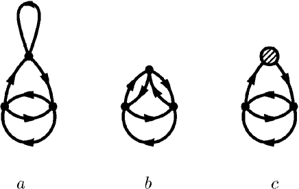
Figure 11: The lowest order three-hole line contributions to the energy of nuclear matter: (a) the third-order bubble diagram, (b) the third order ring diagram, (c) the bubble diagram with an auxiliary potential insertion. The particles above the Fermi sphere propagate from the left to the right, the holes - from the right to the left. The dots denote the $K$-matrix, the shaded vertex - the auxiliary potential $U$.

Given the form of the single particle spectrum, the next natural question is the organization of the diagrams in an expansion which has reasonable convergence properties. The BBG theory identifies such expansion parameter and organizes the diagrams order by order in this small parameter according to the number of independent hole lines (i. e. the number of hole lines that remain after the momentum conservation in a given diagram is taken into account). A diagram with $i$ independent hole lines is of the order of $\kappa^{i-1}$ where the $\kappa$ parameter (pair excitation probability) is defined as

$$\kappa=n\int|\psi(x)-\phi(x)|^{2}d^{3}x,$$ (91)

where $\psi(x)$ is the perturbed pair-wave function satisfying the Schrödinger equation $K\phi=V\psi$, while $\phi(x)$ is the uncorrelated wave function and $n$ is the density. The integral extends to the surface where wave-function restores its free-space form and defines an ‘interaction’ volume $\sim 4\pi\lambda^{3}/3$, where $\lambda$ is the hard-core radius. Thus, we see that $\kappa$ is essentially the ratio of the volumes occupied by the hard-core interaction and a particle. At the saturation density of nuclear matter $\kappa$ is of the order $15\%$, which allows one to estimate the error introduced by neglecting an $i$-hole line diagram to the potential energy

$$\Delta E_{\rm pot}(i)=\Delta E_{\rm pot}(2)\kappa^{i-1}.$$

The expansion clearly breaks down when the interparticle distance is of the order of the hard-core radius of the potential.

The computation of the next-to-leading order three-hole line diagrams is complicated by the fact that the scattering problem of three particles in the nuclear medium needs to be solved. The appropriate equations are due to Bethe and are known as Bethe-Faddeev equations [70]. These equations are the counterparts of the three-body Faddeev equations in the free space, which take into account the influence of the background medium. The lowest order three-hole line diagrams are shown in Fig. 11 [86, 87]. The particles above the Fermi sphere propagate from the left to the right, the holes - from the right to the left. The $K$-matrix is represented by a dot, since the BBG theory assumes $K$ to be local in time. In the case where the spectrum is chosen to have a gap, one needs to evaluate only the diagrams a and b in Fig. 11, while in the case of a continuous spectrum the diagram c in Fig. 11 should be evaluated as well; here the shaded vertex is an insertion of the auxiliary potential $U$. (The rationale behind the gap choice is the cancellation of this type of diagrams in the BBG expansion, albeit, such a choice requires evaluation of the three-hole line diagrams, contrary to the continuous choice which is well converged at the two-hole line level) [88, 89, 90].

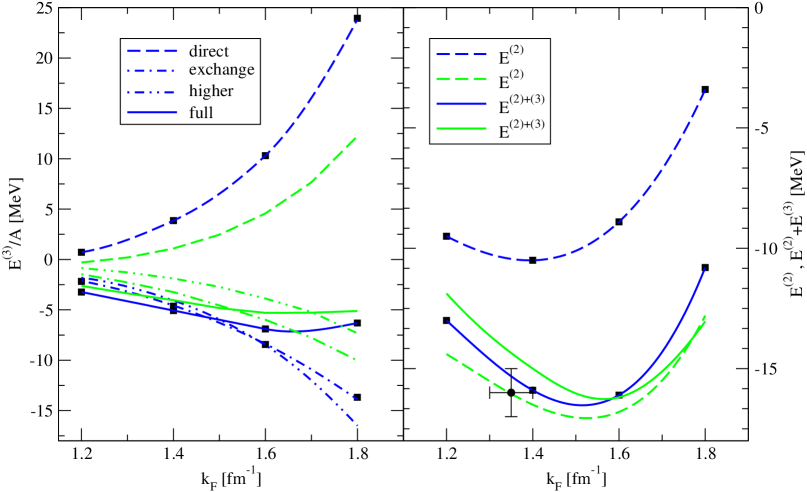
Figure 12: Left panel: The three-hole line contributions to the energy per particle of the isospin symmetrical nuclear matter as a function of the Fermi wave vector. Displayed are the contributions from the direct (dashed line), exchange (dashed-dotted line), higher order (dotted line) diagrams and their sum $E^{(3)}/A$ (solid line). The heavy lines marked with squares show the results obtained with the Reid potential [87, 90] the light lines - with the Argonne V14 potential [88, 89]. Right panel: The energy per particle of isospin symmetrical nuclear matter within the BBG theory. $E^{(2)}$ (dashed line) is the contribution which includes the two-hole line diagrams only; $E^{(2)}+E^{(3)}$ include in addition the three-hole line contributions; the labeling of curves and references are the same as in the left panel, however the results for refs. [88, 89] for the Argonne V14 potential are shown for the continuous spectrum. The empirical saturation point is shown with error bars.

The contribution to the energy from the three-hole line terms can be written, using for simplicity the operator notations, as

$$E^{(3)}=\frac{1}{2}K_{B}\left(\frac{Q_{3}}{{\cal E}_{B}}\right)x{\cal K},$$ (92)

where$x=P_{123}+P_{132}$ and the three-body ${\cal K}$ matrix satisfies the Bethe-Faddeev equation

$${\cal K}=K_{A}x\left(\frac{Q_{3}}{{\cal E}_{B}}\right)K_{B}(1+x)-K_{A}x\left(\frac{Q_{3}}{{\cal E}_{A}}\right){\cal K}.$$ (93)

The first term in Eq. (93) is the sum of the direct ($\propto 1$) and exchange ($\propto x$) diagrams shown in Fig. 11; the second term corresponds to the so-called higher order diagrams. Here the permutation operator is defined as $P|\bm{p}_{3}\bm{p}_{1}\bm{p}_{2}\rangle=|\bm{p}_{1}\bm{p}_{2}\bm{p}_{3}\rangle+|\bm{p}_{2}\bm{p}_{3}\bm{p}_{1}\rangle$, the index $A$ indicates that the spectator third particle is above the Fermi-surface and the index $B$ indicates that there is non. This implies that the matrix elements of the energy denominators in the three-body basis (here $q$ denotes the spectator particle) are defined as

$${\cal E}_{A/B}=\left\{\begin{array}[]{cc}E(\bm{q})+E(\bm{k})+E(\bm{p})-\omega_{3}&({\rm if}~{}~{}q>q_{F},~{}~{}{\rm case~{}A}),\\ E(\bm{k})+E(\bm{p})-\omega_{2}&({\rm if}~{}~{}q<q_{F},~{}~{}{\rm case~{}B}),\end{array}\right.$$ (96)

where $\omega_{3}=E(\bm{p}_{1})+E(\bm{p}_{2})+E(\bm{p}_{3})$ and $\omega_{2}=E(\bm{p}_{1})+E(\bm{p}_{2})$, where $E(\bm{p})$ is the single particle energy. The action of the three-body Pauli operator is written as

$$Q_{3}|\bm{q},\bm{k}\bm{p}\rangle = [1-f_{F}(\bm{k})][1-f_{F}(\bm{p})],\quad\quad f_{F}(\bm{p})\equiv\theta(|p_{F}-p|),$$ (97)

which implies that the particles in the two-body subspace must be outside the Fermi-sphere, while the propagation of the third, spectator particle, is not restricted by the Pauli principle. The BBG Pauli operator should be compared to Eq. (73) which is the most general form of a three-particle Pauli operator for intermediate particle propagation which preserves the particle-hole symmetry.

Fig. 12 shows the various contributions to the three-hole line energy $E^{(3)}$ per particle for several densities parameterized in terms of the Fermi wave vector ($n=2k_{F}^{3}/3\pi^{2}$ in symmetrical nuclear matter). An important feature is the mutual cancellation of the positive contribution from the direct term and the negative contributions from the exchange and higher order terms. The differences between the results of refs. [87, 90] and  [88, 89] shown in the left panel Fig. 12 are due to the differences in the Reid and Argonne V14 potentials. The differences in the right panel are mainly due to the choice of the spectrum - gaped spectrum in the first case and continuous spectrum in the second. The three-hole line contribution to the energy leads to a saturation curve of nuclear matter, which predicts a binding energy that is consistent with the empirical saturation point (Fig. 12, right panel). The minimum of the saturation curve lies at densities that are larger than the empirically deduced one - the missing ingredient is the three-body forces. The convergence of the hole-line expansion in the case of continuous spectrum is faster than in the case of the gaped spectrum; in the first case the two-hole line expansion provides a satisfactory results within the errors which are introduced by ignoring additional physics, such as three-body forces and relativistic dynamics (these two aspects of many body problem cannot be disentangled in general).

2.4 Relativistic $T$-matrix theory

In describing the nuclear phenomenology within relativistic theory two distinct approaches are possible: the phenomenological approach starts with a meson-baryon Lagrangian whose parameters are fitted to reproduce the known empirical properties. A typical set is the binding energy at saturation $E_{B}\simeq-16.0$ MeV, saturation density $\rho_{0}=0.16$ fm^-3, compression modulus $K\sim 300$ MeV, symmetry energy $E_{S}\sim 30$ MeV (see Subsec. 2.5 below) and effective nucleon mass at saturation $m_{N}^{*}=0.8m_{N}$, where $m_{N}$ is the bare nucleon mass [11]. The microscopic approach constructs first the free-space scattering $T$-matrix from a one-boson-exchange potential, which fits to the scattering phase-shifts and the deuteron binding energy; given the free-space interaction a many-body scheme is applied to describe the physics in matter. These models are then extrapolated to the large densities (and temperatures) to describe the properties of matter under stellar conditions. This bottom to top approach (with respect to energy scales) should be contrasted to the top to bottom approaches that attempt to constraint the form of the nucleon-meson Lagrangian and the couplings by the symmetries of the underlying fundamental theory - quantum chromodynamics (QCD). The models that incorporate the chiral symmetry - the dynamical symmetry of strong interactions - are based on low-momentum expansions of chiral Lagrangians; the usefulness of chiral models for treating dense hadronic matter, where momenta are generally not small compared to other relevant scales (e.g. Fermi-energies) is unclear. However, chiral models are useful in treating the meson nucleon interactions in matter; for example, these have been used extensively in the studies of the kaon nucleon interactions in matter [91] (see Subsec. 2.8 for a discussion and Subsec. 2.10 for further references).

2.4.1 Dyson-Schwinger equations and mean field

The elementary constituents of the relativistic models of nuclear matter are the meson and the baryons, whose interaction can be described by a model Lagrangian

$${\cal L}_{I}=-g_{S}\bar{\psi}\psi\phi_{S}-ig_{PV}\bar{\psi}\frac{\gamma^{5}\gamma^{\mu}}{2m_{N}}\psi(\partial_{\mu}\phi_{PV})-g_{V}\bar{\psi}\gamma_{\mu}\psi\phi^{\mu}_{V}-if_{V}\bar{\psi}\frac{\sigma^{\mu\nu}}{2m_{N}}\psi(\partial_{\mu}\phi_{\nu}),$$ (98)

where the $g_{S}$, $g_{V},f_{V}$ and $g_{PV}$ are the coupling constants of the nucleon fields $\psi$ to the meson fields $\phi$, the indices $S$, $V$, and $PV$ refer to scalar, vector and pseudovector couplings. Table 1 lists the (non-strange) mesons, their quantum numbers and typical values of meson-nucleon couplings. The $\sigma$ meson is believed to represent the two-pion exchange contribution to the interaction within the one-boson-exchange models. Chiral symmetry of strong interactions allows the presence of self-interacting meson terms in Eq. (98) which we neglect for simplicity.

meson	$\pi$	$\omega$	$\rho$	$\sigma$	$\eta$	$\delta$	$\phi$
Mass [MeV]	139	784	764	571	550	962	1020
$I,J^{\pi}$	1,0-	0,1-	1,1-	0,0+	0,0-	1, 0+	1-, 0
$g^{2}/4\pi$	14.16	11.7	0.43	7.4	2.0	1.67	-
coupling	$PV$	$V$	$V$	$S$	$PV$	$S$	$V$

Table 1: The masses $M$, the isospin $I$, spin and parity $J^{\pi}$, and couplings $g$ of non-strange mesons. The ratio of the tensor to vector coupling $f/g=0$ for the $\omega$ meson and $5.1$ for the $\rho$ meson.

The Euler-Lagrange equations for the baryon and meson fields lead to the following set of Schwinger-Dyson equations for nucleons

$${\bm{G}}(p) = {\bm{G}}_{0}(p)+{\bm{G}}_{0}(p){\bm{\Sigma}}(p){\bm{G}}(p),$$ (99)

$${\bm{\Sigma}}(p) = -ig_{V}^{2}\int\frac{d^{4}q}{(2\pi)^{4}}\gamma_{\mu}{\bm{D}}_{V}^{\mu\nu}(q){\bm{G}}(p-q){\bm{\Gamma}}_{\nu}(p-q,p;q)$$ (100)

$$- ig_{S}^{2}\int\frac{d^{4}q}{(2\pi)^{4}}{\bm{D}}_{S}(q){\bm{G}}(p-q){\bm{\Gamma}}(p-q,p;q),$$ (101)

$$- ig_{PV}^{2}\int\frac{d^{4}q}{(2\pi)^{4}}\gamma^{5}\gamma_{\mu}\tau^{i}q^{\mu}q^{\nu}{\bm{D}}_{PV}(q){\bm{G}}(p-q){\bm{\Gamma}}^{5j}_{\nu}(p-q,p;q),$$ (102)

where ${\bm{G}}_{0}(p)$ and ${\bm{G}}(p)$ are the free and full nucleon propagators. The summation over the mesons with the same type of coupling is implicit. The nucleon self-energy ${\bm{\Sigma}}(p)$ contains the vector, scalar, and pseudo-vector meson propagators and the associated three-point meson nucleon vertices ${\bm{\Gamma}}(p)$. The meson propagators obey the following Schwinger-Dyson equations, which we write explicitly for the case of vector coupling,

$${\bm{D}}^{\mu\nu}(q) = {\bm{D}}_{0}^{\mu\nu}(q)+{\bm{D}}_{0}^{\mu\lambda}(q){\bm{\Pi}}^{\lambda\rho}(q){\bm{D}}^{\rho\nu}$$ (103)

$${\bm{\Pi}}^{\mu\nu}(q) = -ig_{V}^{2}\int\frac{d^{4}p}{(2\pi)^{4}}{\rm Tr}[\gamma^{\mu}{\bm{G}}(p){\bm{\gamma}}^{\nu}(p,p+q;q){\bm{G}}(p+q)].$$ (104)

The vertices ${\bm{\Gamma}}(p)$ obey their own Schwinger-Dyson equations which connect the three-point functions to four-point and higher order functions. The lowest order truncations of this hierarchy (i. e. replacing the vertices $\Gamma(p)$ by their bare counterparts) leads to the relativistic Hartree and Hartree-Fock theories. Another common approximation is to replace the meson propagators by their free-space counterparts; the resulting nucleon self-energy is written as

$${\bm{\Sigma}}(p) = -ig_{V}^{2}\int\frac{d^{4}q}{(2\pi)^{4}}\left[\gamma_{\mu}\gamma_{\nu}{\bm{D}}_{V}^{\mu\nu}(0){\bm{G}}(q)-\gamma_{\mu}\gamma_{\nu}{\bm{D}}_{V}^{\mu\nu}(q){\bm{G}}(p-q)\right]$$ (105)

$$- ig_{S}^{2}\int\frac{d^{4}q}{(2\pi)^{4}}\left[{\bm{D}}_{S}(0){\bm{G}}(q)-{\bm{D}}_{S}(q){\bm{G}}(p-q)\right]$$

$$- ig_{PV}^{2}\int\frac{d^{4}q}{(2\pi)^{4}}\gamma^{5}\gamma_{\mu}\tau^{i}\gamma^{5}\gamma_{\nu}\tau^{j}q^{\mu}q^{\nu}{\bm{D}}_{PV}(q){\bm{G}}(p-q).$$

Note that pions (which couple by the pseudo-vector coupling) contribute to the self-energy only via the Fock exchange term in last line of Eq. (105). One recovers the conventional relativistic mean field models upon dropping the Fock exchange terms. (It should be noted that the meson self-interactions, which we neglected from the outset, play an important role in the relativistic mean-fields models. The self-interaction coupling provides a further tool for adjusting the models to the phenomenology). The phenomenological models that are based on the Hartree (or Hartree-Fock) description of nuclear matter (the theory is known also as quantum hadrodynamcis) have been used extensively to study the properties of nuclear matter; we will not discuss these models here (see the monographs [11, 12, 92, 93]).

2.4.2 Covariant $T$-matrix

The theories which are based on the covariant treatment of the $T$-matrix and self-energy in nuclear matter are know as the Dirac-Bruckner-Hartree-Fock (DBHF) theories. These theories were developed during the last two decades mostly in the zero-temperature and quasiparticle limits [98, 99, 100, 101, 102, 103, 104, 105, 106, 107, 108, 109, 110]. This section gives a brief overview of the ideas underlying this theory.

We start our discussion of the relativistic $T$-matrix theory by writing down the four-dimension Bethe-Salpeter equation (BSE) in the free space

$$T(p_{1}p_{2};p_{1}^{\prime}p_{2}^{\prime})=V(p_{1}p_{2};p_{1}^{\prime}p_{2}^{\prime})+i\int\frac{d^{4}q}{(2\pi)^{4}}V(p_{1}p_{2};p_{+}^{\prime\prime},p_{-}^{\prime\prime})G_{D}(p_{+}^{\prime\prime})G_{D}(p_{-}^{\prime\prime})T(p_{+}^{\prime\prime},p_{-}^{\prime\prime};p_{1}^{\prime}p_{2}^{\prime}),$$ (106)

where $P=p_{1}+p_{2}$ is the center of mass momentum and $p_{\pm}={P}/{2}\pm p$, and $G_{D}$ is the Dirac propagator

$$iG_{D}(p)=\left[\gamma\cdot p-m+i\eta\right]^{-1}$$ (107)

The reduction of the four-dimensional BSE to the three-dimensional form requires certain constraints on the zero-components of the four-momenta of the in- and outgoing particles. These constraints, the first one due to Gross [94] and the second one due to Logunov-Tavkhelidze [95], Blankenbecler-Sugar [96] and Thompson [97], require that

$$p_{1}^{0}=\sqrt{\bm{p}_{1}^{2}+m^{2}},\quad p_{2}^{0}=\sqrt{s}-p_{1}^{0},$$ (108)

$$p_{1}^{0}=p_{2}^{0}=\frac{\sqrt{s}}{2},$$ (109)

where $s=(p_{1}+p_{2})^{2}$ is one of the Mandelstam invariants. The three-dimensional reduction of the BSE within the Thompson prescription is written as

$$T(\bm{p}_{1}\bm{p}_{2};\bm{p}_{1}^{\prime}\bm{p}_{2}^{\prime};s)=V(\bm{p}_{1}\bm{p}_{2};\bm{p}_{1}^{\prime}\bm{p}_{2}^{\prime})+i\int\frac{d^{4}q}{(2\pi)^{4}}V(\bm{p}_{1}\bm{p}_{2};\bm{p}_{+}^{\prime\prime},\bm{p}_{-}^{\prime\prime})G_{2}(\bm{p}^{\prime\prime},s)T(\bm{p}_{+}^{\prime\prime},\bm{p}_{-}^{\prime\prime};\bm{p}_{1}^{\prime}\bm{p}_{2}^{\prime};s),$$ (110)

where for $\bm{P}=0$ the two-particle propagator is

$$G_{2}(\bm{p},s)=-\frac{m^{2}}{E_{p}^{2}}\frac{\Lambda^{+}(\bm{p})\Lambda^{+}(-\bm{p})}{\sqrt{s}-2E_{p}+i\eta},$$ (111)

where $E_{p}$ is the on-shell particle energy and $\Lambda^{\pm}(\bm{p})$ are the projectors on the positive energy states (the negative energy states are commonly neglected, although a complete analysis of the covariant form of the nucleon-nucleon amplitude requires information for both positive- and negative-energy Dirac spinors [98]).

After the Thompson reduction the interaction is instantaneous, i.e. the retardation effects intrinsic to the full BSE are removed. The reduced relativistic scattering two-body problem is thus described by BSE (110) which permits one to adjust the parameters of the interaction to the experimental phase shifts; the bound state spectrum is described by the homogeneous counterpart of Eq. (110) and can be used to constrain the interactions to reproduce the deuteron binding energy.

Now we turn to the scattering problem in nuclear matter and write the formal solution of the Schwinger-Dyson equation for nucleons as

$$i{\bm{G}}(p)=\left[\gamma\cdot p-m-{\bm{\Sigma}}(p)\right]^{-1}.$$ (112)

The self-energy has a decomposition in terms of the Lorentz invariants

$${\bm{\Sigma}}(p) = {\bm{\Sigma}}_{S}(p)+\gamma_{\mu}{\bm{\Sigma}}_{V}^{\mu}(p)+\frac{\sigma_{\mu\nu}}{2}{\bm{\Sigma}}_{T}^{\mu\nu}(p)+\gamma_{5}{\bm{\Sigma}}_{PS}(p)+\gamma_{5}\gamma_{\mu}{\bm{\Sigma}}_{PV}^{\mu}(p)$$ (113)

$$= {\bm{\Sigma}}_{S}(p_{0},p^{2})+\gamma_{\mu}p^{\mu}{\bm{\Sigma}}_{V}(p_{0},p^{2})+\frac{\sigma_{\mu\nu}}{2}p^{\mu}p^{\nu}{\bm{\Sigma}}_{T}(p_{0},p^{2}).$$

The assumption that the theory is invariant under parity transformations requires that the terms involving $\gamma_{5}$ vanish; the last term in the second line vanishes by the anti-symmetry of the tensor $\sigma_{\mu\nu}$. Since we are interested in the equilibrium properties of matter, we shall not carry along the Schwinger-Keldysh structure and will specify the discussion to the retarded propagators. Upon separating the zero-component of the vector self-energy, $\gamma_{\mu}p^{\mu}{\Sigma}_{V}(p_{0},p^{2})=-\gamma_{0}\Sigma_{0}(p)+{\bm{\gamma}}\cdot\bm{p}\Sigma_{V}(p)$, the propagator (112) can be written as a quasi-free (retarded) propagator

$$iG(p)=\left[\!\not\!p^{\star}-m^{\star}(p)\right]^{-1},$$ (114)

where the effective momenta and masses are defined as

$$m^{\star}(p)=m+{\Sigma_{S}}(p),\quad p_{0}^{\star}=p_{0}+{\Sigma}_{0}(p),\quad\bm{p}^{\star}=\bm{p}\left[1+{\Sigma}_{V}(p)\right];$$ (115)

the analogy to the Dirac propagator is formal because the new quantities are coupled via the self-energies and are complex in general. The form of the new propagator (114) suggests defining effective spinors which are the on-shell positive energy solutions of the medium modified Dirac equation where the imaginary part is set to zero, i. e.

$${u}_{r}(\bm{p})=\left(\frac{E_{p}^{\star}+m^{\star}}{2m^{\star}}\right)^{1/2}\left(\begin{array}[]{c}1\\ {\bm{\sigma}\cdot\bm{p}}{(E_{p}^{\star}+m^{\star})^{-1}}\end{array}\right)\chi_{r},$$ (116)

where $\chi_{r}$ is a state-vector in the spin-space and $E_{p}^{\star}=\sqrt{\bm{p}^{\star 2}+m^{\star 2}}$ is the energy eigenvalue. The effective spinors are normalized according to ${u}_{r}(\bm{p}){u}_{s}(\bm{p})=\delta_{sr}$. For further purposes it is useful to define the effective quantities according to $\tilde{F}(p)=(m^{\star}/E_{p}^{\star})\bar{u}(\bm{p})F(p)u(\bm{p})$. Acting on equation (114) by the unity operator $\Lambda^{+\star}+\Lambda^{-\star}=1$, where the positive and negative energy projectors are defined as $\Lambda^{+\star}={u}_{r}\otimes\bar{u}_{r}$ and upon neglecting the negative energy part one finds

$$\tilde{G}(p)=\left[p_{0}^{\star}-E_{p}^{\star}+i\zeta^{\star}(p)\right]^{-1}.$$ (117)

where the damping is defined as

$$\zeta^{\star}(p)=\mathop{\rm Im}\left[\Sigma_{0}(p)-\frac{m^{\star}}{E_{p}^{\star}}\Sigma_{S}(p)-\frac{p^{\star}}{E_{p}^{\star}}p\Sigma_{V}(p)\right].$$ (118)

The spectral function can be constructed in full analogy to the non-relativistic case

$$\tilde{A}(p)=\frac{\zeta^{\star}(p)}{(p^{\star}-E_{p}^{\star})^{2}+\left[\zeta^{\star}(p)/2\right]^{2}},\quad{\rm lim}_{\zeta^{\star}\to 0}\tilde{A}(p)=2\pi\delta(p^{\star}-E_{p}^{\star}).$$ (119)

The second relation, which corresponds to the quasiparticle limit of the spectral function, defines the single particle energies

$$\varepsilon_{p}=\sqrt{|p^{\star}|^{2}+m^{\star}}-\Sigma_{0}(p).$$ (120)

As in the non-relativistic case, the form of the spectral function is Lorentzian and the spectral sum rule (25) is fulfilled for the general and quasiparticle forms of the spectral function in Eq. (119).

The Bethe-Salpeter equation in the background medium and in the reference frame of the center-of-mass of two particles (suppressing spin indices) is written as

$$T(p,p^{\prime};s^{\star},P)=V(p,p^{\prime})+\int\frac{d^{3}q}{(2\pi)^{3}}V(p,q)\frac{m_{+}^{\star}}{E_{+}^{\star}}\frac{m_{-}^{\star}}{E_{-}^{\star}}\frac{Q_{2}(q,s^{\star},P)}{\sqrt{s^{\star}}-E^{\star}_{+}-E_{-}^{\star}+i\eta}T(q,p^{\prime};s^{\star},P)$$ (121)

where $Q_{2}(q,s^{\star},P)=1-f_{F}(\varepsilon_{P/2+q})-f_{F}(\varepsilon_{P/2-q})$ is the Pauli blocking and $\pm$ is a short hand for $P/2\pm p$. The dependence of the Pauli blocking on $s^{\star}$ and $P$ is due to the function evaluated in the two-particle center-of-mass frame, where the Fermi-sphere is deformed because of Lorentz transformation from the lab to the center of mass frame. A closed set of equations is obtained upon introducing the retarded self-energy in terms of the $T$-matrix (121)

$$\Sigma(p)=\int\frac{d^{3}q}{(2\pi)^{3}}\frac{1}{2E_{q}^{\star}}f_{(1)}^{\alpha}[{\rm Tr}(\!\not\!q^{\star}+m^{\star})f_{(2)}^{\alpha}]T^{\alpha}-(\!\not\!q^{\star}+m^{\star})f_{(2)}^{\alpha}T_{\rm ex}^{\alpha}],$$ (122)

where the subscript ex stands for exchange, $T^{\alpha}$ are coefficients of the expansion of the full $T$-matrix in Lorentz invariants

$$T=\sum_{\alpha}f_{(1)}^{\alpha}f_{(2)}^{\alpha}T^{\alpha},\quad\quad f_{(i)}^{\alpha}\in\{1,\gamma^{\mu}_{i},\sigma^{\mu\nu},\gamma_{5}\gamma^{\mu}_{i},\gamma_{5}\!\not\!q_{i}\}.$$ (123)

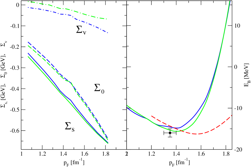
Figure 13: Left panel: The non-vanishing components of the self-energy $\Sigma_{S}$, $\Sigma_{0}$ and $\Sigma_{V}$ as a function of the Fermi-momentum within the Dirac-Brueckner (heavy lines) and the relativistic $T$-matrix (light lines) approximations. Right panel: The binding energy per particle of isospin symmetrical nuclear matter within the Dirac-Brueckner and $T$-matrix theories [102]. The dashed line shows binding energy in a non-relativistic Brueckner theory where the three-body forces are neglected. The empirical saturation point is shown with error bars.

The chemical potential appearing in the Fermi-functions is adjusted to reproduce the density of the system. The solutions of the self-consistent, finite-temperature relativistic $T$-matrix theory allow one to compute the energy density as

$$E=\int\frac{d^{3}p}{(2\pi)^{3}}\left[\langle\bar{u}^{\star}(\bm{p})|{\bm{\gamma}}\cdot\bm{p}+m+\frac{1}{2}\Sigma(\bm{p})|u^{\star}(\bm{p})\rangle\right]f_{F}(\varepsilon_{p}),$$ (124)

and the thermodynamic quantities introduced in Eqs. (42) and (44). The binding energy at zero-temperature [$f_{F}(\varepsilon_{p})\equiv\theta(p_{F}-p)$] is obtained from Eq. (124)

$$E_{B}(p_{F})=\rho^{-1}E(p_{F})-m_{N}.$$ (125)

While we have kept only the positive energy states in our discussion, an unambiguous treatment of the nucleon self-energy in matter requires keeping the negative energy states as well [98, 105, 106]. An example of such an ambiguity is the pion exchange part of the Lagrangian which can be described by a pseudo-scalar or a pseudo-vector coupling. Both couplings produce the same free space matrix elements for the on-shell nucleons when the coupling constants $f_{PV}$ and $g_{PV}$ are related as $f_{PV}/g_{PS}=m_{\pi}/2m$, where $m_{\pi}$ is the pion mass. If only the positive energy states are kept, a recipe to overcome this problem is to divide the $T$-matrix into the Born term plus a correlation term [107, 108]. The ansatz (123) is applied only to the correlation term, since the structure of the Born term is dictated by the interaction $V$, which is fixed.

Another often used approximation is the neglect of the momentum dependence of the self-energies, which are approximated by their value at the Fermi-momentum $p_{F}$. The form of Pauli-operator in Eq. (121) which keeps only the particle-particle propagation in the intermediate state is the counterpart of the non-relativistic Bruckner theory (as it relies on the ideas of the hole-line expansion) [100, 101]. Including the hole-hole propagation leads to the relativistic counterpart of the original $T$-matrix theory [102].

Fig. 13, left panel, shows various components of the nucleon self-energy from a simplest type calculation which ignores the momentum dependence of the self-energies, the negative energy sea and works at zero temperature [102]. The contribution of $\Sigma_{0}$ component is negligible in the case where the negative energy contributions are neglected and the nucleon-nucleon amplitude is expanded according to the ansatz (123). The components $\Sigma_{S}$ and $\Sigma_{0}$ are large on the nuclear scale, but of the same order of magnitude, so that their contributions mutually cancel. The binding energy of isospin symmetrical matter with the Bruckner and $T$-matrix approaches is shown in Fig 13, right panel. The additional density dependence of the Dirac spinors is an important ingredient of the relativistic $T$-matrix theories which leads to a new saturation mechanism. Compared to the non-relativistic theory the saturation density is correctly reproduced by the relativistic theories. The role of the three-body forces within the relativistic theories, in particular the role played by the $\Delta$ isobar, has not been addressed in the literature.

2.5 Isospin asymmetric matter

The proton fraction $Y_{p}$ in neutron star interiors is constrained by the condition of equilibrium with respect to the weak processes. The disparity between the neutron and proton numbers (breaking the $SU(2)$ symmetry in matter) motivates the study of the nuclear matter under isospin asymmetry, which conventionally is described by the asymmetry (or neutron excess) parameter $\alpha=(\rho_{n}-\rho_{p})/(\rho_{n}+\rho_{p})$, where $\rho_{n}$ and $\rho_{p}$ are the number densities of neutrons and protons, or alternatively by the proton fraction $Y_{p}=(1-\alpha)/2.$ The isospin asymmetry is accommodated in the $T$-matrix and related theories by working with two-point functions (self-energies, $T$-matrices etc.) which are $2\times 2$ matrices in the isospin space. The fundamental quantity characterizing the asymmetric nuclear matter is the symmetry energy, $E_{S}$ (i. e. the energy cost of converting a proton into a neutron).

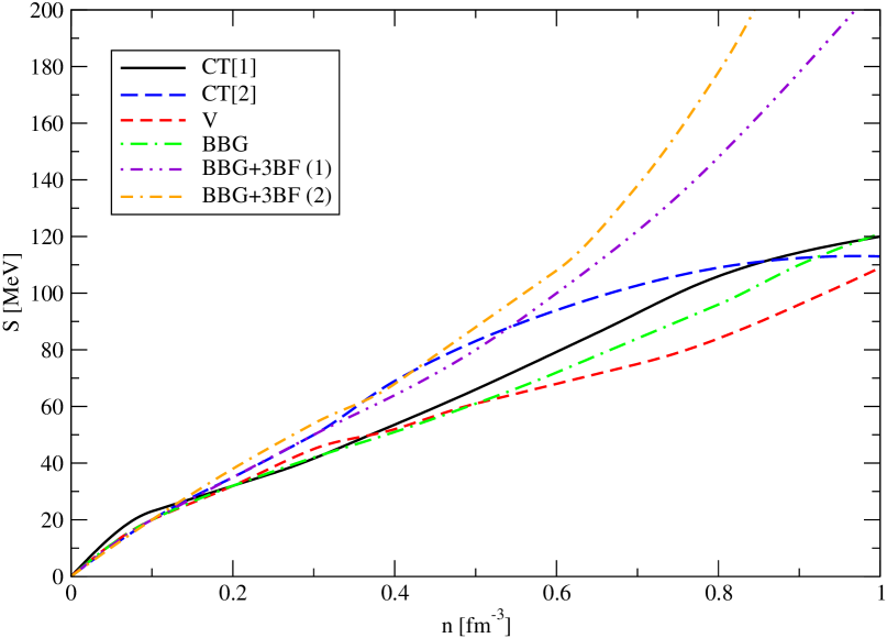
Figure 14: Dependence of symmetry energy of nuclear matter on density. CT[1] and CT[2] refer to the results of refs. [112] and [113] obtained within the covariant $T$-matrix theory. V refers to the variational result of ref. [114] which includes a three-body force; BBG refers to the results based on the BBG theory with two-body forces [115]; BBG(1) includes in addition a microscopically derived three-body force [116, 117, 118]; BBG(2) is the same as BBG(1) but with a phenomenological three-body force [119, 120].

For small values of $\alpha$ the symmetry energy can be expanded in series

$$E_{S}=S_{2}\alpha^{2}+S_{4}\alpha^{4}+O(\alpha^{6}),$$ (126)

where $S_{2}$ is the coefficient in the symmetry energy term of the Bethe-Weizsäcker formula. At zero temperature the contribution from the kinetic energy to $E_{S}$ can be evaluated explicitly in the theories where the matter effects are included in interaction energy alone

$$E_{K}(\rho,\alpha)-E_{K}(\rho,0)=\frac{E_{K}(\rho,0)}{2}\Bigl{\{}\left[(1-\alpha)^{5/3}+(1+\alpha)^{5/3}\right]-1\Bigr{\}}\simeq\frac{5}{9}E_{K}(\rho,0)\alpha^{2}+O(\alpha^{4});$$ (127)

the coefficient of $\alpha^{2}$ identifies the contribution of the kinetic energy to $S_{2}$. The interaction energy contribution is clearly model dependent, in particular it depends on the many-body theory and the nuclear interaction adopted. The importance of studying the symmetry energy arises from the importance of neutron $\beta$-decay reactions in high density matter, whose density threshold depends on the proton concentration (see Subsec 3.1). Some constraints on the symmetry energy can be obtained around the saturation density $\rho_{0}$. An expansion of $S_{2}$ with respect to small deviations from $\rho_{0}$ gives

$$S_{2}(n)=S_{2}(\rho_{0})+\frac{P_{0}}{\rho_{0}^{2}}(\rho-\rho_{0})+O[(\rho-\rho_{0})^{2}].$$ (128)

The first derivative of $S_{2}$ determines the change in the pressure at the saturation point due to the asymmetry of the system. Upon using the expansion (126) one finds [111]

$$P(\rho)=\rho^{2}\frac{\partial E(\rho,\alpha)}{\partial\rho}\simeq P_{0}.$$ (129)

The symmetry energy as a function of density is shown in Fig. 14 for several models which are based on the relativistic Dirac-Bruckner approach [112, 113], variational approach [114] and BBG approach [115]; the latter two approaches include the three-body forces.

The values of the symmetry energy and its derivative at the saturation density vary in a narrow range: $S_{2}(\rho_{0})\simeq 29\pm 2$ MeV and $P_{0}=3\pm 1$ MeV fm³. The predictions of various models of the high density behavour of the symmetry energy differ substantially. The relativistic, variational and BBG theories (the latter without three-body force) vary within $10\%$ of an “average” value. The BBG theories supplemented by either microscopic [116, 117, 118] or phenomenological [119, 120] three-body forces predict symmetry energy that is by a factor of two larger than predictions of other models. However, the discrepancies in the magnitude of the symmetry energy at asymptotically large densities are not essential, since other degrees of freedom such as hyperons, mesonic condensates, or other states of matter are likely to occupy the stable ground state.

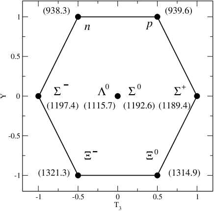
Figure 15: The $SU(3)$ baryon octet. The axis are the isospin $T_{3}$ and the hypercharge $Y$. Baryon masses are given in brackets.

2.6 Hyperons

At densities around the saturation density the only baryonic degrees of freedom are protons and neutrons, which form an iso-duplet whose approximate free-space $SU(2)$ symmetry is largely broken in matter. At larger densities the number of stable baryons increases. These include the isospin 3/2 nucleon resonances $\Delta^{\pm}$, $\Delta^{0}$ and the strangeness carrying baryons (hyperons). The hyperonic states can be classified according to the irreducible representation of the $SU(3)$ group. The two diagonal generators of the group are linear combinations of the isospin $T_{3}$ and hypercharge $Y$, which is equal to the sum of the baryonic number and strangeness, $Y=B+S$. The charges of baryons are determined by the Gell-Mann–Nishijima formula $Q=Y/2+T_{3}$. Fig. 15 shows the octet of the baryons whose strangeness carrying members can appear in neutron star matter. If we neglect the interactions between the hyperons and nucleons, the threshold for hyperons to become stable is determined by comparison of the hyperon mass to the largest available energy scale - the neutron Fermi energy [121]. The $\Sigma^{-}$ hyperons can appear in matter through the weak hyperonic (inverse) beta-decay reactions $e^{-}+n\to\Sigma^{-}+\nu_{e}$ and hadronic weak decay $n+\pi^{-}\to\Sigma^{-}$. The energy balance in the first reaction implies $2\mu_{n}\simeq M_{\Sigma^{-}}=1197$ MeV, where $\mu_{n}$ is the chemical potentials of neutrons (we used the fact that the chemical potential of neutrons and electrons are almost equal in matter under $\beta$ equilibrium, see subsection 2.7). The r. h. side of the second reaction is $O(\mu_{n})$, therefore it is negligible compared to the first reaction. Similar arguments apply to other hyperons which are stabilized either through the hyperonic $\beta$ decays or hadronic weak decays. For example for the lightest hyperon $\Lambda^{0}$ one finds

$$\left.\begin{array}[]{cc}p+e^{-}\to\Lambda^{0}+\nu_{e},\quad p+\pi^{-}\to\Lambda^{0},&O(\mu_{p})\\ n+\pi^{0}\to\Lambda^{0}&O(\mu_{n})\end{array}\right\}=M_{\Lambda}=1116\,\,{\rm MeV}$$ (132)

The reactions in the first line being $O(\mu_{p})$, where $\mu_{p}\ll\mu_{n}$ is the proton chemical potential, can be neglected and $\Lambda^{0}$ appear primarily through the weak hadronic process in the second line. Since the r. h. side of this reaction is $O(\mu_{n})$ and the mass difference $M_{\Sigma^{-}}-M_{\Lambda}<\mu_{n}$ at relevant densities, $\Sigma^{-}$ hyperons appear first.

Interacting hypernuclear matter was initially studied within variational approaches by Pandharipande [131] and Bethe and Johnson [132]. With the advent of the powerful phenomenology of relativistic mean-field models these were extended to the hyperonic sector [133, 134, 135, 136]. The extension of the $T$-matrix and related theories to include hyperons requires the interactions between the hyperons and nucleons ($YN$) and hyperons and hyperons ($YY$) [122, 123, 124, 125]. The experimental information about the interaction involving hyperons is rather scarce. The $YN$ potentials are fitted to the $\Lambda N$ and $\Sigma N$ scattering data. The information on $YY$ interactions is limited to the ground state of double-$\Lambda$ hypernuclei [126]. Additional constraints come from the $SU(3)$ symmetry arguments. The main difference between the $YN$ and the ordinary $NN$ interactions is that the direct $YN$ interaction does not contain the one-pion-exchange (hereafter OPE) part of the $NN$ interaction, therefore the short range part of the nuclear force is not hidden under the dominant OPE interaction. The $\Lambda$ hyperon couples to the neutral pion due to $\Lambda-\Sigma^{0}$ mixing.

The extension of the $T$-matrix theory to include the hyperonic degrees of freedom requires a treatment of the coupled-channel problem. The possible interaction channels in the isospin basis are given in Table 2.

Table 2: The interaction channels within the isospin basis, for combinations of the total strangeness $S$ and total isospin $I$.

	$I=0$	$I={\textstyle\frac{1}{2}}$	$I=1$	$I={\textstyle\frac{3}{2}}$	$I=2$
$S=0$	$N\!N$		$N\!N$
$S=-1$		$(\Lambda N,\Sigma N)$		$\Sigma N$
$S=-2$	$(\Lambda\Lambda,\Xi N,\Sigma\Sigma)$		$(\Xi N,\Sigma\Lambda,\Sigma\Sigma)$		$\Sigma\Sigma$
$S=-3$		$(\Xi\Lambda,\Xi\Sigma)$		$\Xi\Sigma$
$S=-4$	$\Xi\Xi$		$\Xi\Xi$

In the strangeness $S=0,-4$ sectors there is a single channel. In the $S=-1$ sector the channels $\Lambda N,\Sigma N$ are coupled and the $T$-matrix equation reads

$$\left(\begin{array}[]{cc}T_{\Lambda N;\Lambda N}&T_{\Lambda N;\Sigma N}\\ T_{\Sigma N;\Lambda N}&T_{\Sigma N;\Sigma N}\end{array}\right) = \left(\begin{array}[]{cc}V_{\Lambda N;\Lambda N}&V_{\Lambda N;\Sigma N}\\ V_{\Sigma N;\Lambda N}&V_{\Sigma N;\Sigma N}\end{array}\right)$$ (142)

$$+\left(\begin{array}[]{cc}V_{\Lambda N;\Lambda N}&V_{\Lambda N;\Sigma N}\\ V_{\Sigma N;\Lambda N}&V_{\Sigma N;\Sigma N}\end{array}\right)\left(\begin{array}[]{cc}G_{\Lambda N}T_{\Lambda N;\Lambda N}&G_{\Lambda N}T_{\Lambda N;\Sigma N}\\ G_{\Sigma N}T_{\Sigma N;\Lambda N}&G_{\Sigma N}T_{\Sigma N;\Sigma N}\end{array}\right),$$

where the intermediate state propagator, which generalizes the single species result (33) to a multi-component system, is

$$G_{2BB^{\prime}}(\bm{p};P) = \int\!\!\frac{d^{4}P^{\prime}}{(2\pi)^{4}}\int\!\!\frac{d\omega}{(2\pi)}A_{B}(p_{+})A_{B^{\prime}}(p_{-})\left[1-f_{B}(p_{+})-f_{B^{\prime}}(p_{-})\right]\frac{\delta(\bm{P}-\bm{P}^{\prime})}{\Omega-\Omega^{\prime}\pm i\eta},$$ (143)

where $B$ stands for any baryon of the $SU(3)$ octet. The spectral functions in Eq. (143) are related to the self-energies

$$\left(\begin{array}[]{cc}\Sigma^{R}_{\Lambda N}&\Sigma^{R}_{\Sigma N}\\ \Sigma^{R}_{\Sigma N}&\Sigma^{R}_{\Sigma N}\end{array}\right)(p) = \sum_{p^{\prime}}\left(\begin{array}[]{cc}T^{R}_{\Lambda N;\Lambda N}&T^{R}_{\Lambda N;\Sigma N}\\ T^{R}_{\Sigma N;\Lambda N}&T^{R}_{\Sigma N;\Sigma N}\end{array}\right)(p+p^{\prime})\left(\begin{array}[]{cc}G^{<}_{\Lambda N}&G^{<}_{\Lambda N}\\ G^{<}_{\Sigma N}&G^{<}_{\Sigma N}\end{array}\right)(p^{\prime})$$ (155)

$$+\sum_{p^{\prime}}2g(\omega+\omega^{\prime})\left(\begin{array}[]{cc}T^{R}_{\Lambda N;\Lambda N}&T^{R}_{\Lambda N;\Sigma N}\\ T^{R}_{\Sigma N;\Lambda N}&T^{R}_{\Sigma N;\Sigma N}\end{array}\right)(p+p^{\prime}){\rm Im}\left(\begin{array}[]{cc}G^{R}_{\Lambda N}&G^{R}_{\Lambda N}\\ G^{R}_{\Sigma N}&G^{R}_{\Sigma N}\end{array}\right)(p^{\prime}).$$

Equations (142) and (155) are the generalization of the equations of (32) and (41) to the case of coupled $\Lambda N,\Sigma N$ channels. The example above is sufficiently general to illustrate the treatment of other coupled channels shown in Table 2. The Brueckner-Bethe-Goldstone theory for hyperonic matter is recovered from the above equations by (i) taking the quasiparticle and zero temperature limits and (ii) dropping the hole-hole propagation from the intermediate state propagators.

The BBG calculations of hypernuclear matter were carried out over several decades in parallel to the development of the theory for ordinary nuclear matter with a special attention to the problem of binding of $\Lambda$ particle in nuclear matter (see e.g. [127, 128, 129, 130]). Recent work on Bruckner theory for hypernuclear matter shifted the interest towards understanding the $\beta$-equilibrated matter in neutron stars [137, 138, 139, 140] (see Subsec. 2.9 below).

2.7 Charge neutrality and weak equilibrium

Neutron stars evolve towards equilibrium with respect to the weak interactions on long time scales. However, in many cases, the time-scales of interest are much shorter than these equilibration time-scale and we can assume, to a good approximation, that the NS interiors are in approximate weak equilibrium between hadrons and leptons. If the temperatures in the interiors of NS are below several MeV, which corresponds to time scales of the order of months or less after star’s formation, the neutrinos propagate through the star without interactions. Their chemical potentials can be set to zero. In a matter composed of neutrons ($n$), protons $(p)$ and electrons $(e)$ the weak equilibrium is established by the $\beta$-decay and electron capture reactions

$$n\to p+e^{-}+\bar{\nu}_{e},\quad\quad p+e^{-}\to n+\nu_{e}.$$ (156)

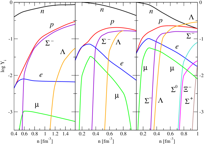
Figure 16: Matter composition in $\beta$-equilibrated hypernuclear matter. Left panel: Noninteracting matter [121]; Central panel: Interacting mixture according to the BBG theory [140]; Right panel: Interacting mixture within a relativistic mean-field theory [133].

The equilibrium condition requires that the chemical potentials obey the equality $\mu_{e}=\mu_{n}-\mu_{p}.$ Given the energy density of asymmetric nuclear matter $\varepsilon$ the chemical potentials can be expressed as

$$\mu_{n/p}=\frac{\partial\varepsilon}{\partial n_{n/p}}=\frac{\partial\varepsilon}{\partial n}+\frac{1\mp\alpha}{n}\frac{\partial\varepsilon}{\partial\alpha},\quad\delta\mu=\frac{2}{n}\frac{\partial\varepsilon}{\partial\alpha},$$ (157)

where $\delta\mu=\mu_{n}-\mu_{p}=\mu_{e}$. The charge neutrality requires that the number densities $n_{p}=n_{e}$; treating electrons as a non interacting and massless $n_{e}=\mu_{e}^{3}/3\pi^{2}$, which in turn implies that

$$Y_{p}=Y_{e}=\frac{8}{3\pi^{2}n}\left(\frac{\partial\varepsilon}{\partial n}\right)^{3}=\frac{8}{3\pi^{2}n}S_{2}^{3}\left(\frac{1}{2}-Y_{p}\right)^{3}\quad(\mu_{e}\geq m_{\mu}),$$ (158)

where in the last step the expansion (126) has been used. Eq. (158) allows one to compute the proton fraction at a given density if the symmetry coefficient $S_{2}$ is known. When the electron chemical potential exceeds the muon rest mass $m_{\mu}=105.7$ MeV the electrons decay into muons via the reaction

$$e^{-}\to\mu^{-}+\bar{\nu}_{\mu}+\bar{\nu}_{e}.$$ (159)

Equilibrium with respect to this process and its inverse requires $\mu_{e}=\mu_{\mu}$, where $\mu_{\mu}$ is the chemical potential of muons. The proton fraction in this case is given by the parametric equation

$$Y_{p}=\frac{1}{3\pi^{2}n}\left[(\delta\mu^{2}-m_{\mu}^{2})^{3/2}+\delta\mu^{3}\right].$$ (160)

The conditions for $\beta$-equilibrium and charge neutrality are readily generalized to the case of arbitrary numbers of baryons and leptons; the key observation is that there are two conserved charges available - the total baryonic charge, which is related to the conservation of the baryonic density and the total electrical charge, which is related to the charge neutrality of matter. The thermodynamic potential of matter is a functional of the baryon $n(Y_{i})$ and lepton $n(Y_{j})$ densities, where $i$ and $j$ enumerate the baryon and lepton species respectively:

$$\Omega(Y_{i},Y_{j})=E-\mu_{B}\left[n_{B}-\sum_{i}B_{i}Y_{i}n\right]-\mu_{L}n\left[\sum_{i}Q_{i}Y_{i}+\sum_{j}Q_{j}Y_{j}\right],$$ (161)

where $B_{i}$ and $Q_{i}$ are the baryon and electric charges and $\mu_{B}$ and $\mu_{L}$ are the associated Lagrange multipliers, $n_{B}$ is the baryon density. The equilibrium conditions require

$$\frac{\partial\Omega}{\partial Y_{i}}=0,\quad\frac{\partial\Omega}{\partial Y_{j}}=0.$$ (162)

The baryon and lepton chemical potentials are obtained as

$$\mu_{i}=\frac{\partial E}{\partial Y_{i}}=-\mu_{B}B_{i}+\mu_{L}Q_{i},\quad\quad\mu_{j}=\frac{\partial E}{\partial Y_{j}}=\mu_{L}Q_{j}.$$ (163)

If the neutron and electron chemical potentials are chosen as independent parameters, Eqs. (163) identify $\mu_{B}=-\mu_{n}$ and $\mu_{e}=-\mu_{L}$ and the chemical potentials of arbitrary baryonic species are written as $\mu_{i}=B_{i}\mu_{n}-Q_{i}\mu_{e}$. For example for a mixture consisting of $n$, $p$, $\Sigma^{\pm}$ and $\Lambda^{0}$ baryons the equilibrium conditions give

$$\mu_{\Sigma^{-}}=\mu_{n}+\mu_{e},\quad\mu_{\Lambda}=\mu_{n},\quad\mu_{\Sigma^{+}}=\mu_{n}-\mu_{e}=\mu_{p},\quad\mu_{\mu}=\mu_{e},$$ (164)

$$Y_{p}+Y_{\Sigma^{+}}-(Y_{e}+Y_{\mu}+Y_{\Sigma^{-}})=0.$$ (165)

Fig. 16 shows the abundances of various species in a baryon-lepton mixture within the non-interacting hyperonic matter theory [121], BBG theory [140] and the relativistic mean-field theory [133]. The interacting models agree qualitatively at low densities, however at larger densities the relativistic theory allows for the $\Sigma^{0,+}$ hyperons and the cascade $\Xi^{-}$.

2.8 Meson condensation

Bose-Einstein condensation (BEC) of mesons has an important impact on the properties of hadronic matter in NS. First, it softens the equation of state and, second, it leads to an enhanced neutrino emission. Contrary to the ordinary Bose-Einstein condensation, where above the critical temperature one deals with a normal Bose gas, the pion condensation is associated with an unstable mode in nuclear matter which has the quantum numbers of pions (ref. [141] and references therein). The threshold of pion condensation is derived by considering the pion retarded propagator in nuclear medium

$$D_{\pi}(\omega,\bm{q})=\left[\omega^{2}-\bm{q}^{2}-m_{\pi}^{2}-\Pi(\omega,\bm{q})\right]^{-1},$$ (166)

where the pion self-energy, which is represented by the polarization tensor of nuclear matter $\Pi(\omega,\bm{q})$, sums the particle-hole ($ph$) and $\Delta$-resonance – hole ($\Delta h$) states to all orders. [The equations determining the pion propagator and the self-energy are identical to Eqs. (103) and (104) with the vector coupling replaced by the pseudo-vector coupling.] The resummation of these channels in nuclear matter is a complex problem in general [142, 143], but can be performed analytically if one approximates the driving term in the $ph$ and $\Delta h$ series by Landau parameters

$$\Gamma_{ph}=f+g~{}\bm{\sigma}_{1}\cdot\bm{\sigma}_{2}+(f^{\prime}+g^{\prime}~{}\bm{\sigma}_{1}\cdot\bm{\sigma}_{2})(\bm{\tau}_{1}\cdot\bm{\tau}_{2}),$$ (167)

where $\bm{\sigma}$ and $\bm{\tau}$ are the vectors of Pauli matrices in spin and isospin spaces. In analogy to (167) one may define the interaction in the $\Delta h$ channel as $\Gamma_{\Delta h}=g^{\prime}_{N\Delta}(\bm{\sigma}_{1}\cdot{\bf S}_{2})(\bm{\tau}_{1}\cdot{\bf T}_{2})$ and $\Gamma_{\Delta\Delta}=g^{\prime}_{\Delta\Delta}({\bm{S}}_{1}\cdot{\bm{S}}_{2})({\bm{T}}_{1}\cdot{\bm{T}}_{2}),$ where ${\bm{S}}$ and ${\bm{T}}$ are the spin and isospin operators for the $\Delta$ resonance. The net polarization tensor is the sum of nucleon and $\Delta$ contributions, $\Pi=(\omega^{2}-\bm{q}^{2})\tilde{\chi}_{N}+\bm{q}^{2}f\tilde{\chi}_{\Delta}$, where $f=\left[(m_{N}+m_{\Delta})^{2}-(\omega^{2}-\bm{q}^{2})\right]/4m_{\Delta}^{2}$, with $m_{N}$ and $m_{\Delta}$ being the nucleon and $\Delta$-resonance mass. The “susceptibilities” which include the effects of short-range correlations are given in terms of one-loop Lindhard functions $\chi_{N}$ and $\chi_{\Delta}$ as [144]

$$\tilde{\chi}_{N}=[1+(g^{\prime}_{\Delta\Delta}-g^{\prime}_{N\Delta})\chi_{\Delta}]{\cal D}^{-1},\quad\tilde{\chi}_{N}=[1+(g^{\prime}_{NN}-g^{\prime}_{N\Delta})\chi_{\Delta}]{\cal D}^{-1},$$ (168)

where ${\cal D}=1+g^{\prime}_{NN}\chi_{N}+g^{\prime}_{\Delta\Delta}\chi_{\Delta}+(g^{\prime}_{NN}g^{\prime}_{\Delta\Delta}+g_{N\Delta}^{{}^{\prime}2})\chi_{N}\chi_{\Delta}$. Due to the isospin symmetry of nuclear matter the polarization tensors of neutral and charged pions are equivalent. Their spectral function can be written as

$$B_{\pi}(\omega,\bm{q})=\frac{-2{\rm Im}\Pi^{R}(\omega,\bm{q})}{[\omega^{2}-\bm{q}^{2}-m_{\pi}^{2}-{\rm Re}\Pi^{R}(\omega,\bm{q})]^{2}+[{\rm Im}\Pi^{R}(\omega,\bm{q})]^{2}}.$$ (169)

The pion condensation in symmetric nuclear matter is characterized by the condition $B(0,\bm{q}_{c})\to\infty$ at ${\rm Im}\Pi^{R}(0,\bm{q}_{c})\to 0$. In the presence of $\pi$ condensate the uniform nuclear matter acquires a periodic nucleonic spin wave structure with wavenumber $\bm{q}_{c}$. These qualitative features remain intact for neutral pion condensation in neutron matter. Charged pion condensation in neutron matter is characterized by additional instabilities. Apart from the collective modes mentioned above, a mode appears which carries the quantum numbers of $\pi^{+}$ above some critical density $\rho_{+}$, which depends on the details of the repulsive interaction in the $S=1$ and $T=1$ channel. In terms of nucleon excitations it represents a bound state of a proton and a neutron hole. At higher densities the sum of the poles of the $\pi^{+}$ and $\pi^{-}$ propagators [c. f. Eq. (166)] vanishes, which signals the instability of matter towards formation of $\pi^{-}\pi^{+}$ meson pairs.

Whether the pion condensation occurs in compact stars is an open issue. The answer depends crucially on the values of the $g^{\prime}$ parameters; the currently accepted range of $g^{\prime}_{NN}\in 0.6-0.8$ and the universality ansatz, which sets all the $g^{\prime}$ parameters equal to $g_{NN}^{\prime}$, precludes pion condensation in finite nuclei and in compact stars within the density range where the nucleonic and mesonic components retain their identity. Recent analysis of Gamow-Teller resonance in the ⁹⁰Zr(p,n)⁹⁰Nb reaction [145] suggests the following values of parameters: $g^{\prime}_{NN}=0.59$ and $g^{\prime}_{N\Delta}=0.18+0.05g^{\prime}_{\Delta\Delta}$, with $g^{\prime}_{\Delta\Delta}$ being undetermined. With this new information the critical density of pion condensation turns out to be lower than that with the universality ansatz [146]. An independent evidence for low-density neutral pion condensation was obtained in variational calculations of ref. [114].

The mechanism by which kaons may from a Bose condensate in neutron star matter was developed by Kaplan and Nelson [91]. Since the anti-kaon interactions in nuclear matter are attractive, their effective mass could be substantially lower than their mass in the vacuum. Thus, instead of neutralizing the positive charge by the negative charge of energetic electrons, this can be done by stabilizing $K^{-}$ in matter. Most of the effects of $K^{-}$ condensation on the properties of compact stars are similar to those discussed for pion condensation. These include a substantial softening of the equation of state which reduces the maximum mass of a compact star to $1.5M_{\odot}$. This reduction may have important implications for the low-mass black hole population in our Galaxy [147].

2.9 Stellar models

The equilibrium configurations of compact stars are described by the Einstein equations of General Theory of Relativity (GTR)

$$R_{ik}-\frac{1}{2}Rg_{ik}=\frac{8\pi k}{c^{4}}T_{ik}\quad i,k=0,1,2,3$$ (170)

where $R_{ik}$ is the Ricci tensor, $R$ - the scalar curvature, $g_{ik}$ - the metric tensor, $T_{ik}$ - the energy-momentum tensor and $k$ - the Newton’s constant; the cosmological constant is omitted from the Einstein’s equations. The gravitational field created by a spherically symmetric mass distribution is itself spherically symmetric. For such fields the components of the metric tensor are functions of the radial coordinate $r$ and time $t$. The metric can be written

$$ds^{2}=e^{\nu}c^{2}dt^{2}-e^{\lambda}dr^{2}-r^{2}(d\theta^{2}+{\rm sin~{}}^{2}\theta d\phi^{2}).$$ (171)

The energy and momentum tensor can be expressed through the mass density $\rho$ and pressure $P$ as

$$T_{ik}=(\rho+c^{-2}P)u_{i}u_{k}-Pg_{ik},$$ (172)

where $u_{i}$ is the matter four-velocity. For a static mass distribution $T_{0}^{0}=\rho c^{2}$ and $T_{1}^{1}=T_{2}^{2}=T_{3}^{3}=-P$. In the static (time-independent) limit and for spherically symmetric gravity Eq. (170) reduces to

$$e^{-\lambda}\left(\frac{\lambda^{\prime}}{r}-\frac{1}{r^{2}}\right)+\frac{1}{r^{2}} = \frac{8\pi k}{c^{2}}\rho$$ (173)

$$e^{-\lambda}\left(\frac{\nu^{\prime}}{r}+\frac{1}{r^{2}}\right)-\frac{1}{r^{2}} = \frac{8\pi k}{c^{4}}P$$ (174)

$$\frac{1}{2}e^{-\lambda}\left(\nu^{\prime\prime}+\frac{\nu^{{}^{\prime}2}}{2}+\frac{\nu^{\prime}-\lambda^{\prime}}{r}-\frac{\nu^{\prime}\lambda^{\prime}}{2}\right) = \frac{8\pi k}{c^{4}}P,$$ (175)

where primes denote radial derivatives. The last equation can be replaced by the equation for hydrodynamic equilibrium

$$P^{\prime}+\frac{1}{2}(P+c^{2}\rho)\nu^{\prime}=0,$$ (176)

which is nothing else than the explicit form of the covariant hydrodynamic equations $T^{n}_{m;n}=0.$ Eqs. (173), (174), and (176) should be supplemented with the equation of state $P(\rho)$ and boundary conditions $P(0)$, $\nu(0)$ and $\lambda(0)$. The inner solution within the configuration should be matched with the external Schwarzschild solution

$$e^{\nu}=e^{-\lambda}=1-\frac{2kM}{c^{2}r},$$ (177)

where $M$ is the mass of the configuration. The quantity $R_{S}={2kM}/{c^{2}}$ is the Schwarzschild radius; the importance of general relativity is determined by the ratio $R_{S}/R$ where $R$ is a characteristic length (e.g. the star radius).

It is evident that at the center of the configuration $\lambda(0)=0$, $\lambda^{\prime}(0)=\nu^{\prime}(0)=0$ to avoid singularities as $r\to 0$. The problem of finding the internal solutions of stellar configurations is simplified upon introducing a new variable via the relation $e^{-\lambda}=1-{2km(r)}/{c^{2}r}$. One finds [148]

$$\frac{dm(r)}{dr} = 4\pi\rho r^{2},$$ (178)

$$\frac{dP}{dr} = -\frac{k(P+c^{2}\rho)}{[c^{2}r-2km(r)]r}\left[m(r)+\frac{4\pi}{c^{2}}Pr^{3}\right].$$ (179)

Thus we have two equations for three variable $p$, $\rho$, and $m$. The system of equations is closed by specifying the equation of state $P(\rho)$. We implicitly assumed that the pressure is independent of temperature, as is the case for a system at zero temperature. However in those cases where the temperature is important, the complete set of equations includes apart from the equation of state also two new differential equations which describe the energy balance and thermal transport equations (see Chapt. 4.2).

To gain insight in the equations of hydrostatic equilibrium (178) and (179) consider a self-gravitating star with constant density $\rho_{0}$. Integrating the first equation gives $m(r)=4\pi\rho_{0}r^{3}/3.$ The integration of the second equation gives

$$r=R_{0}\left[1-\left(\frac{3P+c^{2}\rho_{0}}{P+c^{2}\rho_{0}}\frac{P_{0}+c^{2}\rho_{0}}{3P_{0}+c^{2}\rho_{0}}\right)^{2}\right]^{1/2},\quad R_{0}=\left(\frac{3c^{2}}{8\pi k\rho_{0}}\right)^{1/2}.$$ (180)

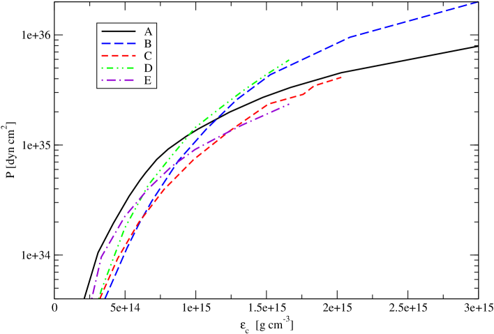
Figure 17: Pressure vs central energy density for representative equations of state (EoS). Model A (solid line) - relativistic mean field model, features hyperons and pion condensate [133]. Model B (dashed line) - non-relativistic variational EoS based on AV14 potential supplemented by UVII three-body force [149]. Model C (short dashed line) - relativistic model based on covariant $T$-matrix [112]. Model D (dashed double-dotted) - non-relativistic EoS based on the BBG theory, includes a three-body force. Model E (dashed dotted) - same as model D, but includes interacting hyperons [140].

Substituting $P=0$ one finds the radius $R$ of the configuration. The metric within the sphere is written as

$$e^{-\lambda}=1-\frac{r^{2}}{R_{0}^{2}},\quad e^{\nu}=\left(1-\frac{2kM}{c^{2}R}\right)\left(\frac{c^{2}\rho_{0}}{c^{2}\rho_{0}+P(r)}\right)^{2},\quad r\leq R.$$ (181)

These solutions match the Schwarzschild solution (177) at the surface of the configuration. For the constant density $\rho_{0}=2.85\times 10^{14}$ g cm^-3 and maximal pressure $P=5\times 10^{33}$ erg cm^-3 one finds the maximal radius and the mass of the configuration: $R=6.4$ km, $M=0.16~{}M_{\odot}$. In the case of an incompressible fluid $P(r)/c^{2}\rho_{0}=1/3$ and one finds $R=17.74$ km, $M=3.3~{}M_{\odot}$. The numbers above give approximate lower and upper limits on the mass and radius of a compact object. For a more realistic estimate we now turn to the many-body equations of state of hadronic matter.

EoS	method	composition	forces
A	RMF	$npeH\pi$	contact 2B
B	variational	$npe$	realistic 2B + 3B
C	DBHF	$npe$	realistic 2B
D	BBG	$npe$	realistic 2B + 3B
E	BBG	$npeH$	realistic 2B + 3B

Table 3: Summary of EoS A-E introduced in the text; $H$ refers to hyperons, $\pi$ – pion condensate, $2B$ and $3B$ – two and three-body forces, RMF – relativistic mean field. The remaining abbreviation are introduced in the text.

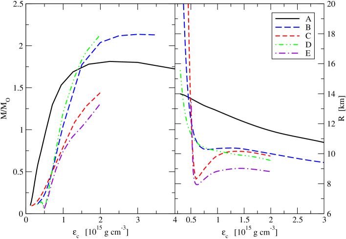
Figure 18: Left panel: Dependence of the gravitational mass (in units of solar mass $M_{\odot}$) on the central energy density for configurations constructed from EoS A-E specified in the text. Right panel: Dependence of the star’s radius on its central density for EoS A-E.

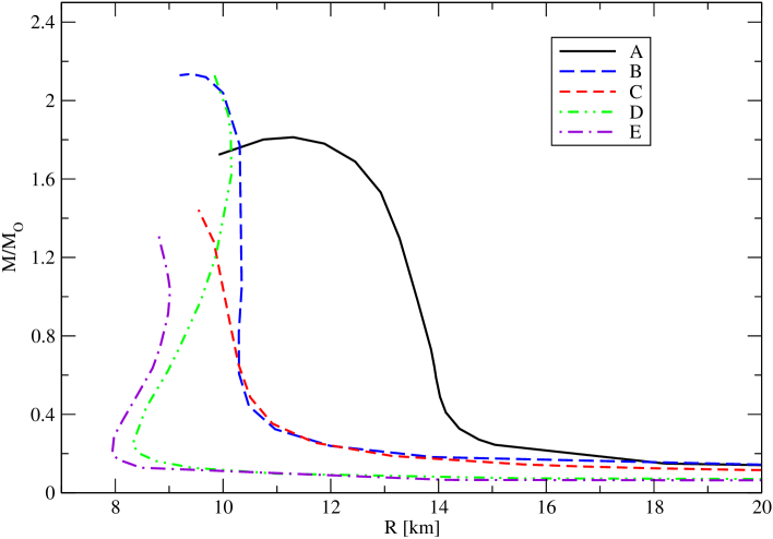
Figure 19: Dependence of configuration masses on their radii for EoS A-E specified in the text.

For illustrative purposes we have chosen several equations of states which are either based on the theories discussed in previous sections or are alternatives listed in Subsec. 2.10; their properties are summarized in Table 3. Dependence of pressure on central density for models labeled A-E are shown in Fig. 17. Model A is a relativistic mean field model which allows for hyperons and onset of pion condensation [133]. Model B is a non-relativistic variational model based on the Argonne AV14 two-body potential which is supplemented by the Urbana UVII three-body force [149]. Model C is a covariant model based on the Dirac-Bruckner (covariant $T$-matrix) theory [112]. Finally, models D and E are based on the BBG theory which employs two-body and three body forces [140]. Model E includes hyperons along with the nucleonic component, whose interactions are taken into account within the BBG theory.

Equations of state are commonly characterized by their stiffness, which is expressed through the adiabatic index $\gamma={\rm log}P/{\rm log}\rho$ (the larger the adiabatic the stiffer the equation of state). The non-relativistic models B and D which include only nucleonic component interacting with two- and three-body forces are the stiffest equations of state at large densities. The relativistic mean field model A is stiff at low densities where the hyperons are still not present but becomes softer at higher densities as the result of hyperonization of matter and pion condensation. As a general trend new degrees of freedom soften the equation of state since the new constituents of matter share the stress due to the pressure with other constituents. Such a softening is apparent from a comparison of non-relativistic models D and E which differ by the presence of hyperons in the latter model. Note that the models are shown in their published density range. They were supplemented by the equations of state for low-density matter from refs. [150] and [151] to construct sequences of stellar models.

The masses and radii for sequences of configurations with different central energy densities $\varepsilon_{c}$ are shown in Fig. 18 for equations of state (hereafter EoS) A to E. The configurations were computed with the RNS code written by Stergioulas [152]. As a common trend one finds that the stiffer is the EoS at the central density of a configuration, the larger is its mass. Each configuration features a maximal mass, but because of the limited density range across which our models are defined this mass is apparent only for models A, B and D . Mass measurements of compact stars obtained from the timing of binary pulsars are broadly consistent with a canonical mass of 1.4 $M_{\odot}$. Pulsars that have undergone long periods of accretion have larger masses. The most massive measured pulsar to date PSR J0751+1807 is a millisecond pulsar in a 6hr binary system with a helium white dwarf secondary. The mass of the pulsar is measured through the orbital decay which is interpreted as due to emission of gravity waves. Combined with measurements of the Shapiro delay, this implies a pulsar mass $2.1\pm 0.2$ $M_{\odot}$ [153]. While models A-D feature stars with canonical masses of 1.4 $M_{\odot}$ (an exception is the model E), the latter observation places a severe limit on the EoS of nuclear matter and excludes all the models except B and D. Recent observations of binary pulsars that have undergone extended periods of accretion without losing their stability indicate that the EoS of compact stars ought to be rather stiff. All except the lightest members of the sequences shown in Fig. 19 are characterized by small radii which are confined within the range of 8-11 km, their value being almost independent of the central energy density (see Fig. 18). This leads to degeneracy in the mass-radius relationship in Fig. 19: for models B, D and E there exist configurations with different masses but same radii.

EoS	$\varepsilon_{c}$	$M$	$R$	$\Omega_{K}$	$P_{K}$	$T/W$	$cJ/kM_{\odot}^{2}$	$I$
	[1015 g/cm3]	$M_{\odot}$	[km]	[$10^{4}$ s-1]	[$10^{-3}$ s]			$[10^{45}$ g cm${}^{2}]$
A	4.00	1.98	13.1	1.05	0.60	0.088	2.32	1.94
B	2.00	2.50	12.9	1.20	0.52	0.145	4.53	3.29
C	2.00	1.77	12.9	1.03	0.61	0.118	2.08	1.77
D	1.60	2.49	13.5	1.14	0.55	0.181	4.67	3.62
E	1.60	1.47	12.8	0.97	0.64	0.200	1.55	1.41

Table 4: Parameters of compact stars rotating at their Keplerian frequency constructed from EoS A-E specified in the text. The models listed are the largest mass (stable) configuration for the EoS A and B and the largest central density configuration for EoS C-D. The entries are the central energy density, the gravitational mass, the equatorial radius, the Keplerian rotation frequency and period $P_{K}=2\pi/\Omega_{K}$, the ratio of the kinetic (rotational) to the potential (gravitational) energy, the angular momentum $J$, and the moment of inertia $I$.

Apart from the stationary global observable like the mass and radius, stellar configurations are characterized by the dynamical quantities such as the moment of inertia $I$, rotational angular momentum $J$ and limiting rotation frequency $\Omega_{K}$, know as the Kepler frequency. The rotation of the star modifies the metric and thus the rotation frequency in the local inertial frame, which we denote by $\omega_{L}$. Slowly rotating stars admit perturbative approach, where the small parameter is the ratio of the rotational kinetic energy to the gravitational binding energy [154, 155, 156, 157, 158, 159]. The angular velocity of a slowly rotating star obeys the following equation

$$(r^{4}j\omega_{L}^{\prime})^{\prime}+4r^{3}j^{\prime}\omega_{L}=0,\quad\quad j=e^{-(\nu+\lambda)/2}.$$ (182)

The external solution of Eq. (182) is given by

$$\omega_{L}(r)=\Omega-\frac{2kJ}{c^{2}r^{3}}$$ (183)

where $\Omega$ is the rotation frequency. The internal solution can be obtained through integration of Eq. (182) with the boundary conditions $\omega_{L}^{\prime}=0$, when $r=0$ and $j(r)=1$ when $r=R$. The moment of inertia for slowly rotating objects can be written as

$$I=\frac{J}{\Omega}=\frac{8\pi}{3}\int_{0}^{R}dr~{}r^{4}e^{(\lambda-\nu)/2}\left(\rho+\frac{P}{c^{2}}\right)\frac{\omega_{L}}{\Omega},$$ (184)

where the volume integration assumes approximate spherical symmetry. The Keplerian frequency $\Omega_{K}$ is defined as the frequency at which the centrifugal force on a test particle at the equator equals the gravitational binding force. For rotational frequencies $\Omega>\Omega_{K}$ mass shedding from the equator leads to instability of the configuration. Table 4 lists the parameters of the general relativistic configurations rotating at the Kepler frequency. The values of the central density correspond either to the maximum mass stable (non-rotating) configuration (models A, B) or the largest central density available for a given EoS (models C-E). N. B. The central densities of these configurations exceed the nuclear saturation density by factors of the order of 10. It is likely that the baryonic and mesonic degrees of freedom are not appropriate at such large densities; nevertheless the EoS of quark matter can not differ dramatically from those listed above, and the conclusions drawn from the limiting frequencies should hold, at least qualitatively. The fastest millisecond pulsar measured to date is IGR J00291+5934 with rotation period $P=1.7$ ms. According to Table 4 and the studies of limiting frequencies of rotating superdense stars based on alternative EoS (ref. [12], Chapter 16), stars that are gravitationally bound can not rotate faster than half a millisecond. The situation is different if a configuration is self-bound due to strong interactions, as is the case for the strange stars. Thus, if an object is observed in the future with rotation periods smaller than half a millisecond it must be an exotic object, e.g. a compact star made up of strange matter (ref. [12], Chapter 18).

2.10 A guide to alternative methods

Here we complement the discussion of the nuclear many-body problem above by a brief summary of some of the alternative methods that are used in the studies of the nuclear many-body problem.

Qunatum Monte Carlo (QMC) methods have been used extensively to study the properties of infinite nuclear matter, neutron matter and light nuclei with various versions of the Argonne two-body and the Urbana three-body interactions (ref. [160] and references therein). Recent developments include calculations of the ground state energy of nuclear and neutron matter using the Argonne AV18 and Urbana UIX potentials [114], Green’s functions Monte-Carlo (GFMC) calculations of light nuclei [161], and QMC calculations of neutron matter [162, 163, 164]. These calculations are variational in nature (i. e. provide an upper bound on the energy of the system) and are based on a non-relativistic description of nucleonic matter in terms of the Schrödinger equation.

Chiral Perturbation theory seeks to establish a connection between non-perturbative QCD and low-energy phenomenology of nuclear systems. This top to bottom (with regard to the energy scales) approach is anchored in the symmetries of the QCD Lagrangian (notably the approximate chiral symmetry of strong interactions) and in the QCD sum rules. In the nuclear and neutron matter problems the chiral perturbation theory offers a method of treating the long-range pion-nucleon dynamics explicitly, the short-range correlations being incorporated in contact terms [165, 166, 167, 168]. As mentioned in Subsec. 2.8, chiral Lagranians are useful in deriving the properties of the kaon condensate in dense matter. Furthermore, chiral Lagrangians have been used to derive free-space nucleon-nucleon interactions that are input in many-body and few-body calculations (ref. [169] and references therein).

Relativistic density functional theories are based on the ideas of the mean-field theory of nucleons and mesons. These models incorporate a limited number of phenomenological constants, that are fitted to the properties of bulk nuclear matter and finite nuclei, and provide a powerful tool to study many aspects of nuclear phenomenology at an elementary (Hartree or Hartree-Fock) level [170]. Some recent models incorporate the chiral symmetry in the Lagrangian of the theory [171, 172, 173].

Lattice field theory methods have gained attention in recent years. The nuclear and neutron matter problems were studied in close analogy to the numerical simulations of the Hubbard model in condensed matter systems [174, 175, 176]. Lattice methods were also applied to dilute, spin 1/2 non-relativistic fermions [177]. A lattice realization of the scalar $\phi^{6}$ field theory was applied to study $\alpha$ clusters in nuclear matter [178].

During the past decade the Effective field theory methods were developed for nuclear systems and applied to the few-body nuclear physics; see refs. [182, 183, 184] and references therein. Some aspects of the many-body problem are discusses within this method in refs. [185, 186].

Coupled cluster method is one of the most powerful and universally applicable techniques in quantum many-body theory, that is well suited for treating non-perturbative problems. Its application to the nuclear many-body problem and finite nuclei has a long history (see ref. [179] and references therein). Recent developments include the quantum chemistry inspired coupled cluster calculations of ground and excited states of nuclei [180, 181].

3 Neutrino interactions in dense matter

The temperature of a NS born in a supernova explosion is of the order of several tens of MeV. During the first seconds neutrinos are trapped inside the star (i.e. the neutrino mean free path $\lambda_{\nu}\ll R$, where $R$ is the star radius). The energy that is lost in neutrinos is radiated from the surface of the neutrino-sphere - the surface where the optical depth for neutrinos drops to zero. Once the star cools down to temperatures of the order of several MeV, the matter becomes transparent to neutrinos ($\lambda_{\nu}\gg R$). The subsequent thermal evolution of NS is controlled by neutrino radiation from its interiors for the following $10^{3}$-$10^{4}$ years. This long term evolution of NS is independent of the cooling history during the first several hours when the interior cools down to temperatures of the order of 0.1 MeV. The thermal history of NS does strongly depend on the neutrino emission rates from dense matter during the neutrino radiation epoch $t\leq 10^{4}-10^{5}$ years. The neutrino emission rates in turn depend crucially on matter composition, elementary particle content, and condensed matter properties, such as superfluidity and superconductivity. Thus the studies of thermal evolution of neutron stars offer a unique tool to test the physics of neutron star interiors. The measurements of the surface temperatures of young NS by $X$-ray satellites have the potential of constraining the properties of dense matter. The late-time $t\geq 10^{5}$ thermal evolution of NS is dominated by cooling via the photoemission from the surface and heating due to conversion of rotational and magnetic energy into heat. This chapter reviews the neutrino radiation processes that are relevant for the neutrino radiation era.

3.1 Classification of weak processes

We start with a classification of the weak reactions and concentrate first on the nucleonic matter. It is useful to classify the processes by the number of baryons in the initial (or final) state. The simplest neutrino emission process that involves single baryon in the initial (final) state are

$$n\to p+e+\bar{\nu},\quad p+e\to n+\nu,$$ (185)

$$n\to n+\nu+\bar{\nu}\hskip 142.26378pt({\rm forbidden}).$$ (186)

The first reaction is the charge current $\beta$-decay (and its inverse). It is known in astrophysics as the Urca processes [187]. The Urca reaction is kinematically allowed in matter under $\beta$-equilibrium if the proton fraction is sufficiently large [188, 189]. The threshold for the Urca process arises from the kinematical requirement of simultaneous conservation of momentum and energy in the reaction; a simple estimate for cold matter in $\beta$-equilibrium shows that the proton fraction $Y_{p}\geq 11-14\%$ for the Urca process to work [189, 190].

The second process - the neutral current neutrino pair bremsstrahlung is forbidden by the energy and momentum conservation. This statement is true if $n$ refers to (quasi)particles whose spectral function is a delta function [cf. Eq. (45)]. If one chooses to work with excitations that are characterized by finite widths, the reaction (186) is allowed [191]. The point is that the finite width incorporates multi-particle processes that we are going to include explicitly in the next to leading order of expansion. The process with two baryons in the initial (and final) states are the modified Urca and its inverse [192, 193]

$$n+n\to n+p+e+\bar{\nu},\quad p+n\to p+p+e+\bar{\nu},$$ (187)

$$n+p+e\to n+n+\nu,\quad p+p+e\to p+n+\nu.$$ (188)

and the modified bremsstrahlung processes

$$N+N\to N+N+\nu+\bar{\nu},\quad N\in n,p.$$ (189)

The modified processes are characterized by a spectator baryon that guarantees the energy and momentum conservation in the reaction. We can continue adding further spectator baryons on both sides of the reactions above, however the power radiated by higher order reactions drops dramatically for two reasons. First, if we consider the three-body processes, which are next in the hierarchy, the probability of scattering of three quasiparticles is suppressed compared to the two-body counterpart (Pauli principle). Second, adding an extra fermion in the initial and final state introduces a small factor $T/E_{F}\ll 1$ for each fermion, where $E_{F}$ is the Fermi energy. Thus, going one step higher in the hierarchy suppresses the reaction rate by a small parameter $(T/E_{F})^{2}$. The relevant quantity for numerical simulations of neutron star cooling is the neutrino emissivity, which is defined as the power of energy radiated per unit volume. The emissivities of the processes above are $\varepsilon_{\beta}\sim 10^{27}\times T_{9}^{6}$ for the reaction (185), $\varepsilon_{mod.~{}\beta}\sim 10^{21}\times T_{9}^{8}$ for the reactions (187) and (188), and $\varepsilon_{\nu\bar{\nu}}\sim 10^{19}\times T_{9}^{8}$ for the reactions (189); here $T_{9}$ is the temperature in units $10^{9}$ K.

The general arguments above apply to the reactions in the hypernuclear matter under $\beta$-equilibrium (Subsection 2.6). The charge current processes on hyperons (hyperon Urca processes) are

$$\Sigma^{-}\to n+e+\bar{\nu},\quad\quad\left(\begin{array}[]{c}\Lambda^{0}\\ \Sigma^{0}\end{array}\right)\to\left(\begin{array}[]{c}p\\ \Sigma^{+}\end{array}\right)+e+\bar{\nu},\quad\quad\left(\begin{array}[]{c}\Sigma^{-}\\ \Xi^{-}\end{array}\right)\to\left(\begin{array}[]{c}\Lambda^{0}\\ \Sigma^{0}\\ \Xi^{0}\end{array}\right)+e+\bar{\nu}$$ (190)

and the reactions inverse to these. Note that some of the reaction involve violation of strangeness conservation by weak interactions with a change of strangeness by amount $\Delta S=1$. The neutrino emissivity of the hyperon Urca process has the same parametric dependence on the density of states and temperature as the nucleonic Urca process, however it is smaller than the nucleonic Urca process because the weak matrix elements are suppressed by factors of 0.01 - 0.6. Another important difference is that the threshold for the $\Lambda^{0}\to pe\bar{\nu}$ reaction, corresponding to the $\Lambda^{0}$ hyperon fraction $Y_{\Lambda}\simeq 0.0013$, is much smaller than the threshold for the process (185) [194]. The remainder reactions have similar thresholds as the ordinary Urca and, being less effective, contribute a fraction of the total emissivity. The pair bremsstrahlung processes (186) on hyperons need to conserve the strangeness and are forbidden at the one-body level. The modified Urca processes involving hyperons can be written as [195]

$$B_{1}+B_{2}\to B_{3}+B_{2}+e+\bar{\nu},$$ (191)

with the baryons $B_{i}$ $(i=1,2,3)$ chosen consistent with charge conservation; the strangeness is either conserved or changed by amount $\Delta S=1$. The inverse of (191) yields the same result as the direct reaction. The modified bremsstrahlung process can be written as [195]

$$B_{1}+B_{2}\to B_{3}+B_{4}+\nu+\bar{\nu},$$ (192)

where the weak interaction vertex, written symbolically as $B\to B+\nu+\bar{\nu}$, involves arbitrary octet baryons. (Note that contrary to ref. [195], current work finds non-vanishing matrix elements for the $\Lambda\to\Lambda+\nu+\bar{\nu}$ transition within the $SU(6)$ quark model for the baryon octet [196]). The estimates of the reactions (191) and (192) which are based on the one-pion-exchange (OPE) potential show that the emissivities of hyperonic processes are small compared to their nucleonic counterparts, contributing at most 2/3 of the total nucleonic emissivity. The OPE interaction adequately represents only the long-range part of the interaction. The short range repulsive components of the nuclear force reduces the rate of neutrino emission by modified processes by factors 4-5; since the reduction applies to the entire baryon octet the relative ratio of the nucleonic to hyperonic emissivities should not be affected. The exchange of strangeness carrying mesons, such as the $K$-meson, opens new channels for hyperonic modified processes and this will enhance the contribution of hyperons to the cooling rate.

We mentioned above that the reaction (186) is forbidden for quasiparticles with $\delta$-function type spectral functions (45) by the energy and momentum conservation. This constraint is lifted in the case where the baryons pair [197, 198, 199]. The binding energy of Cooper pairs makes it energetically possible to create $\nu\bar{\nu}$ pairs in the inelastic processes of pair creation and annihilation:

$$B(\Delta)\to B(\Delta)+\nu+\bar{\nu},$$ (193)

where $B(\Delta)$ is a quasiparticle excitation of the superfluid state. The rate of the Cooper pair breaking and formation (CPBF) processes is of the order of ($10^{19}-10^{21})\times T_{9}^{7}$ depending on the baryon pairing patterns [197, 198, 199]. At extreme low temperature these processes are suppressed exponentially as ${\rm exp}(-\Delta(0)/T)$, where $\Delta(0)$ is the zero-temperature pairing gap.

The neutral current one-body process (193) induced by the superfluidity have their charge current counterparts [200]. While the former vanish when the temperature approaches the critical temperature of superfluid phase transition, the emissivity of the latter process approaches the value of the corresponding Urca process. Put another way, the suppression of the Urca processes in the superfluid state is not restricted to the reduction of the phase space; the pair breaking can take place for these processes as well. In the extreme low temperature limit the Urca processes are suppressed exponentially as ${\rm exp}(-\Delta_{\rm max}(0)/T)$, where $\Delta_{\rm max}(0)$ is the largest gap for fermions involved in the reaction. The modified processes are suppressed by factors ${\rm exp}\{-[\Delta_{B}(0)+\Delta_{B^{\prime}}(0)]/T\}$ where $B$ and $B^{\prime}$ label the pair of the initial or final baryons. As in the case of the Urca process the largest gaps enter the suppression factor.

If pions or kaons form a Bose-Einstein condensate (BEC) the meson decay reactions contribute via the reactions [201]

$$n+\langle\pi^{-}\rangle\to n+e^{-}+\bar{\nu}_{e},$$ (194)

$$n+\langle K^{-}\rangle\to n+e^{-}+\bar{\nu}_{e}.$$ (195)

The emissivities of these reactions are large compared to those of the baryonic processes above; for pions $\varepsilon_{\pi}\sim 10^{26}T_{9}^{6}$ and for kaons $\varepsilon_{K}\sim 10^{25}T_{9}^{6}$; thus, a distinctive property of the models that feature a meson condensate is the rapid cooling. Note the kinematical differences in these reactions, since pions condense at finite momentum and in the $P$-wave, while kaons form a zero momentum condensate in the $S$-wave.

3.2 Transport equations for neutrinos

This section introduces the real-time formalism for neutrino transport [202]. We shall treat neutrinos as massless particles, since on the energy scales relevant for neutron star physics the masses of neutrinos are small. For massless neutrinos it is irrelevant whether neutrinos are Dirac or Majorana particles and their free particle Lagrangians are identical. The interaction Lagrangian for the charge current is

$${\cal L}_{W}=\frac{g_{W}}{\sqrt{2}}\sum_{a}\left(L^{-}_{a\mu}W^{-\mu}+L^{+}_{a\mu}W^{+\mu}\right),\quad L^{-}_{a\mu}=\bar{\psi}_{La}^{\nu}\gamma_{\mu}\psi_{La}^{l},\quad L^{+}_{\mu a}=\bar{\psi}_{La}^{l}\gamma_{\mu}\psi_{La}^{\nu},$$ (196)

where $g_{W}$ is charge current coupling constant, $W^{\pm}$ are the gauge vector boson fields, $L^{\pm}_{a\mu}$ is the lepton current written in terms of left-handed chiral spinors of neutrino $\psi_{aL}^{\nu}$ and lepton $\psi_{aL}^{l}$, $a$ is the flavor index. The interaction Lagrangian for the charge neutral interaction is

$${\cal L}_{Z}=\frac{g_{Z}}{{2}}\sum_{a}\left(J_{a\mu}Z^{\mu}+J^{f}_{a\mu}Z^{\mu}\right),\quad J_{a\mu}=\bar{\psi}_{La}^{\nu}\gamma_{\mu}\psi_{La}^{\nu},\quad J^{f}_{\mu a}=\bar{\psi}_{a}^{f}\gamma_{\mu}(c_{v}-c_{A}\gamma^{5})\psi_{a}^{f},$$ (197)

where $g_{Z}=g_{W}/{\rm cos~{}}\theta_{W}$, where $\theta_{W}=28.7^{o}$, ${\rm sin~{}}^{2}\theta_{W}=0.23$. These coupling constants are related to the Fermi coupling constant by the relation $G_{F}=(1/\sqrt{2})(g_{W}/2M_{W})^{2}=1.166\times 10^{-5}$ GeV^-2, where $M_{W}\simeq 82$ GeV is the $W$-boson mass (the $Z$-boson mass $M_{Z}=M_{W}/{\rm cos~{}}\theta_{W}$).

The theory of neutrino radiation can be conveniently formulated in terms of the real-time quantum neutrino transport, as discussed in Section 2. The neutrino Greens functions are written in the matrix form

$$i{\bm{S}}(1,2)=i\left(\begin{array}[]{cc}S^{c}(1,2)&S^{<}(1,2)\\ S^{>}(1,2)&S^{a}(1,2)\end{array}\right)=\left(\begin{array}[]{cc}\left<T\psi(1)\bar{\psi}(2)\right>&-\left<\bar{\psi}(2)\psi(1)\right>\\ \left<\psi(1)\bar{\psi}(2)\right>&\left<\tilde{T}\psi(1)\bar{\psi}(2)\right>\end{array}\right),$$ (198)

where $\psi(1)$ are the neutrino field operators, $\bar{\psi}=\gamma^{0}\psi^{*}$, $T$ is the chronological time ordering operator, and $\tilde{T}$ is the anti-chronological time ordering operator; the indexes $1,2,\dots$ denote the space-time arguments. The neutrino matrix propagator obeys the Dyson equation

$${\bm{S}}(1,2) = {\bm{S}}_{0}(1,2)+{\bm{S}}_{0}(1,3){\bm{\Omega}}(3,2){\bm{S}}(2,1),$$ (199)

where ${\bm{S}}_{0}(1,2)$ is the free neutrino propagator and ${\bm{S}}_{0}^{-1}(1,2){\bm{S}}_{0}(1,2)=\sigma_{z}\delta(1-2)$, $\sigma_{z}$ is the third component of the (vector) Pauli matrix, ${\bm{\Omega}}$ is the neutrino proper self-energy and we assume integration (summation) over the repeated variables. The self-energy ${\bm{\Omega}}$ is a $2\times 2$ matrix with elements defined on the contour.

The set of the four Green’s functions above can be supplemented by the retarded and advanced Green’s functions which are defined, in analogy to (10) and (11), as

$$iS^{R}(1,2)=\theta(t_{1}-t_{2})\langle\left\{\psi(1),\overline{\psi}(2)\right\}\rangle,\quad iS^{A}(1,2)=-\theta(t_{2}-t_{1})\langle\left\{\psi(1),\overline{\psi}(2)\right\}\rangle,$$ (200)

where $\{\,,\,\}$ stands for an anti-commutator. The retarded and advanced Green’s functions obey integral equations in the quasiclassical limit. By applying the Langreth-Wilkins rules (15) and (16) to the Dyson equation (199) we find the transport equation for the off-diagonal elements of the matrix Green’s function

$$\left[\not\!\partial_{3}-\mathop{\rm Re}\,\Omega^{R}(1,3),S^{>,<}(3,2)\right]-\left[\mathop{\rm Re}\,S^{R}(1,3),\Omega^{>,<}(3,2)\right]$$

$$\hskip 85.35826pt=\frac{1}{2}\left\{S^{>,<}(1,3),\Omega^{>,<}(3,2)\right\}+\frac{1}{2}\left\{\Omega^{>,<}(1,3),S^{>,<}(3,2)\right\},$$ (201)

where $[\,,\,]$ stands for commutator. In arriving at Eq. (201) we assumed the existence of the Lehmann representation for the neutrino propagators; as a result we find $\mathop{\rm Re}~{}S^{R}=\mathop{\rm Re}~{}S^{A}\equiv\mathop{\rm Re}~{}S$ and $\mathop{\rm Re}~{}\Omega^{R}=\mathop{\rm Re}~{}\Omega^{A}\equiv\mathop{\rm Re}~{}\Omega$.

The neutrino dynamics can be treated semiclassically, by separating the slowly varying center-of-mass coordinates from the rapidly varying relative coordinates. Carrying out a Fourier transform with respect to the relative coordinates and keeping the first-order gradients in the slow variable we arrive at a quasiclassical neutrino transport equation

$$i\left\{\mathop{\rm Re}S^{-1}(q,x),S^{>,<}(q,x)\right\}_{P.B.}+i\left\{\mathop{\rm Re}\,S(q,x),\Omega^{>,<}(q,x)\right\}_{P.B.}$$

$$\hskip 85.35826pt=S^{>,<}(q,x)\Omega^{>,<}(q,x)+\Omega^{>,<}(q,x)S^{>,<}(q,x),$$ (202)

where $q\equiv(\bm{q},q_{0})$ and $x$ are the neutrino four momentum and the center-of-mass space-time coordinate, respectively, $\{\dots\}_{P.B.}$ is the four-dimensional Poisson bracket [cf. Eq. (27)]. To eliminate the second Poisson bracket on the l. h. side of Eq. (202) we carry out a decomposition analogous to (23) with respect to the small neutrino damping: $S^{>,<}(q,x)=S_{0}^{>,<}(q,x)+S_{1}^{>,<}(q,x)$, where $S_{0}^{>,<}(q,x)$ is the leading (quasi-particle) and $S_{1}^{>,<}(q,x)$ is the next-to-leading order term. The quasiparticle part of the transport equation is then written as  [202]

$$i\left\{\mathop{\rm Re}S^{-1}(q,x),S_{0}^{>,<}(q,x)\right\}_{P.B.}=S^{>,<}(q,x)\Omega^{>,<}(q,x)+\Omega^{>,<}(q,x)S^{>,<}(q,x)$$ (203)

and describes the evolution of the distribution function (Wigner function) of on-shell excitations. The l. h. side of Eq. (203) corresponds to the drift term of the Boltzmann equation, while the r. h. side corresponds to the collision integral, where the self-energies $\Omega^{>,<}(q,x)$ are interpreted as the collision rates. The advantage of this form of the (generalized) collision integral is that it admits systematic approximations in terms of the Feynman perturbation theory. The remainder part of the transport equation

$$i\left\{\mathop{\rm Re}S^{-1}(q,x),S_{1}^{>,<}(q,x)\right\}_{P.B.}+i\left\{\mathop{\rm Re}\,S(q,x),\Omega^{>,<}(q,x)\right\}_{P.B.}=0,$$ (204)

relates the off-mass-shell part of the neutrino propagator to the self-energies in a form of a local functional which depends on the local (anti-)neutrino particle distribution function and their coupling to matter.

3.2.1 On-shell neutrino approximation

The on-mass-shell neutrino propagator is related to the single-time distribution functions (Wigner functions) of neutrinos and anti-neutrinos, $f_{\nu}(q,x)$ and $f_{\bar{\nu}}(q,x)$, via the ansatz

$$S_{0}^{<}(q,x) = \frac{i\pi\!\not\!q}{\omega_{\nu}(\bm{q})}\Big{[}\delta\left(q_{0}-\omega_{\nu}(\bm{q})\right)f_{\nu}(q,x)-\delta\left(q_{0}+\omega_{\nu}(\bm{q})\right)\left(1-f_{\bar{\nu}}(-q,x)\right)\Big{]},$$ (205)

where $\omega_{\nu}(\bm{q})=|q|$ is the on-mass-shell neutrino/anti-neutrino energy. Note that the ansatz includes simultaneously the neutrino particle states and anti-neutrino hole states, which propagate in, say, positive time direction. Similarly, the on-shell propagator

$$S_{0}^{>}(q,x) = -\frac{i\pi\!\not\!q}{\omega_{\nu}(\bm{q})}\Big{[}\delta\left(q_{0}-\omega_{\nu}(\bm{q})\right)\left(1-f_{\nu}(q,x)\right)-\delta\left(q_{0}+\omega_{\nu}(\bm{q})\right)f_{\bar{\nu}}(-q,x)\Big{]},$$ (206)

corresponds to the states propagating in the reversed time direction and, hence, includes the anti-neutrino particle states and neutrino hole states.

To recover the Boltzmann drift term, we take the trace on both sides of the transport equation (202) and integrate over the (anti-)neutrino energy $q_{0}$. The single time Boltzmann equation (hereafter BE) for neutrinos is obtained after integrating over the positive energy range:

$$\left[\partial_{t}+\vec{\partial}_{q}\,\omega_{\nu}(\bm{q})\vec{\partial}_{x}\right]f_{\nu}(\bm{q},x)=\int_{0}^{\infty}\frac{dq_{0}}{2\pi}{\rm Tr}\left[\Omega^{<}(q,x)S_{0}^{>}(q,x)-\Omega^{>}(q,x)S_{0}^{<}(q,x)\right];$$ (207)

a similar equation follows for the anti-neutrinos if one integrates in Eq. (202) over the range $[-\infty,0]$.

The different energy integration limits select from the r. h. side of the transport equations the processes leading to modifications of the distribution functions of (anti-)neutrinos. The separation of the transport equation into neutrino and anti-neutrino parts is arbitrary. It is motivated by the observation that the fundamental quantities of neutrino radiative transport, as the energy densities or neutrino fluxes, can be obtained by taking the appropriate moments of BEs and these quantities are not symmetric with respect to the neutrino/anti-neutrino populations in general.

3.2.2 Collision integrals

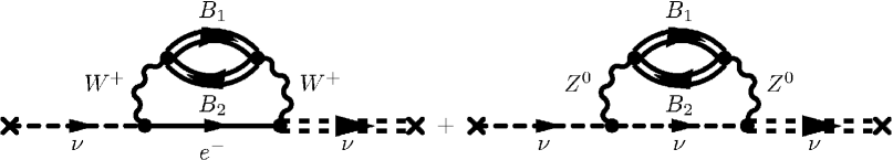
Figure 20: The neutrino self-energies for charge and neutral current processes. The dashed and double-dashed curves correspond to the free and full neutrino propagators (reverting the time-direction one finds the propagators for anti-neutrinos). The solid line is the electron propagator. The loop is the baryon polarization tensor involving baryons $B_{1}$ and $B_{2}$. The wavy lines correspond to the $W^{+}$ and $Z^{0}$ boson propagators. The incoming and outgoing $\nu$ propagators are shown for clarity and are not included in the self-energy.

The diagrams contributing to the neutrino emission rates can be arranged in a perturbation expansion with respect to the weak interaction. The lowest order in the weak interaction Feynman diagrams which contribute to scattering, emission, and absorption processes are shown in the Fig. 20. The corresponding transport self-energies are read-off from the diagram

$$-i\Omega^{>,<}(q_{1},x) = \int\frac{d^{4}q}{(2\pi)^{4}}\frac{d^{4}q_{2}}{(2\pi)^{4}}(2\pi)^{4}\delta^{4}(q_{1}-q_{2}-q)i\Gamma_{L\,q}^{\mu}\,iS_{0}^{<}(q_{2},x)i\Gamma_{L\,q}^{\dagger\,\lambda}i\Pi^{>,<}_{\mu\lambda}(q,x),$$ (208)

where $\Pi^{>,<}_{\mu\lambda}(q)$ are the off-diagonal elements of the matrix of the baryon polarization tensor, $\Gamma_{L\,q}^{\mu}$ is the weak interaction vertex. The contact interaction can be used for the energy-momentum transfers much smaller than the vector boson mass, $q\ll M_{Z},M_{W}$, in which case the gauge boson propagators are approximated as

$$iD_{Z,W}=\frac{g_{\mu\nu}-q_{\mu}q_{\nu}/M_{Z,W}^{2}}{q^{2}-M_{Z,W}^{2}}\simeq-\frac{g_{\mu\nu}}{M_{Z,W}^{2}},$$ (209)

where $g_{\mu\nu}$ is the metric tensor. Let us first concentrate on the BE for neutrinos. Define the loss and gain terms of the collision integral as:

$$I_{\nu}^{>,<}(\bm{q},x)=\int_{0}^{\infty}\frac{dq_{0}}{2\pi}{\rm Tr}\left[\Omega^{>,<}(q,x)S_{0}^{>,<}(q,x)\right].$$ (210)

Substituting the self-energies and the propagators in the collision integrals we find for, e.g., the gain part:

$$I_{\nu}^{\rm<}(\bm{q}_{1},x) = -i\int_{0}^{\infty}\frac{dq_{10}}{2\pi}{\rm Tr}\Biggl{\{}\int_{-\infty}^{\infty}\frac{d^{4}q}{(2\pi)^{4}}\frac{d^{4}q_{2}}{(2\pi)^{4}}(2\pi)^{4}\delta^{4}(q_{1}-q_{2}-q)\Gamma^{\mu}_{L}\frac{\pi\!\not\!q_{2}}{\omega_{\nu}(\bm{q}_{2})}\Big{[}\delta\left(q_{02}-\omega_{\nu}(\bm{q}_{2})\right)f_{\nu}(q_{2},x)$$

$$- \delta\left(q_{02}+\omega_{\nu}(\bm{q}_{2})\right)\left(1-f_{\bar{\nu}}(-q_{2},x)\right)\Big{]}\Gamma^{\dagger\,\lambda}_{L}\frac{\pi\!\not\!q_{1}}{\omega_{\nu}(\bm{q}_{1})}\delta\left(q_{10}-\omega_{\nu}(\bm{q}_{1})\right)\left(1-f_{\nu}(q_{1},x)\right)\Pi_{\mu\lambda}^{>}(q,x)\Biggr{\}}.$$

The loss term is obtained by replacing in Eq. (3.2.2) the neutrino Wigner functions by the neutrino-hole functions $f_{\nu}(q,x)\to(1-f_{\nu}(q,x))$ and the anti-neutrino-hole Wigner functions by the anti-neutrino functions $\left(1-f_{\bar{\nu}}(-q,x)\right)\to f_{\bar{\nu}}(q,x)$. The terms proportional $(1-f_{\nu})f_{\nu}$ and $(1-f_{\nu})(1-f_{\bar{\nu}})$ in the gain part of the collision integral, $I_{\nu}^{<}(\bm{q})$, correspond to the neutrino scattering-in and emission contributions, respectively. The terms proportional $f_{\nu}(1-f_{\nu})$ and $f_{\nu}f_{\bar{\nu}}$ in the loss part of the collision integral, $I_{\nu}^{>}(\bm{q})$, are the neutrino scattering-out and absorption contributions.

The loss and gain collision integrals for the anti-neutrinos can be defined in a manner, similar to the case of neutrinos, with the energy integration spanning the negative energy range

$$I_{\bar{\nu}}^{>,<}(\bm{q},x)=\int^{0}_{-\infty}\frac{dq_{0}}{2\pi}{\rm Tr}\left[\Omega^{>,<}(q,x)S_{0}^{>,<}(q,x)\right].$$ (212)

Using the above expressions for the self-energy and the propagators, we find, e.g., for the gain term:

$$I_{\bar{\nu}}^{<}(\bm{q}_{1},x) = i\int^{0}_{-\infty}\frac{dq_{10}}{2\pi}{\rm Tr}\Biggl{\{}\int_{-\infty}^{\infty}\frac{d^{4}q}{(2\pi)^{4}}\frac{d^{4}q_{2}}{(2\pi)^{4}}(2\pi)^{4}\delta^{4}(q_{1}-q_{2}-q)\Gamma^{\mu}_{L}\frac{\pi\!\not\!q_{2}}{\omega_{\nu}(\bm{q}_{2})}\Big{[}\delta\left(q_{02}-\omega_{\nu}(\bm{q}_{2})\right)f_{\nu}(q_{2},x)$$ (213)

$$- \delta\left(q_{02}+\omega_{\nu}(\bm{q}_{2})\right)\left(1-f_{\bar{\nu}}(-q_{2},x)\right)\Big{]}\,\Gamma^{\dagger\lambda}_{L}\frac{\pi\!\not\!q_{1}}{\omega_{\nu}(\bm{q}_{1})}\delta\left(q_{10}+\omega_{\nu}(\bm{q}_{1})\right)f_{\bar{\nu}}(-q_{1},x)\Pi^{>}_{\mu\lambda}(q,x)\Biggr{\}}.$$

The loss term is obtained by making replacements in Eq. (213) analogous to those applied to Eq. (3.2.2). The terms proportional $f_{\nu}f_{\bar{\nu}}$ and $f_{\bar{\nu}}(1-f_{\bar{\nu}})$ in the gain part of the collision integral, $I_{\bar{\nu}}^{<}(\bm{q})$, then correspond to the neutrino absorption and scattering-out contributions. The terms proportional $(1-f_{\bar{\nu}})(1-f_{\nu})$ and $(1-f_{\bar{\nu}})f_{\bar{\nu}}$ in the loss part of the collision integral, $I_{\bar{\nu}}^{>}(\bm{q})$, are the neutrino emission and scattering-in contributions, respectively. Note that, when the neutrinos are in thermal equilibrium with the baryons, the collision integrals for the scattering-in/scattering-out and for the absorption/emission cancel. Under the conditions of detailed balance the (anti-)neutrino distribution function reduces to the Fermi-Dirac form.

3.2.3 Neutral current processes (bremsstrahlung)

The neutrino-pair emissivity (the power of the energy radiated per volume unit) is obtained by multiplying the left-hand-sides of the neutrino and anti-neutrino by their energies, respectively, summing the BEs, and integrating over a phase space element:

$$\epsilon_{\nu\bar{\nu}} = \frac{d}{dt}\int\!\frac{d^{3}q}{(2\pi)^{3}}\left[f_{\nu}(\bm{q})+f_{\bar{\nu}}(\bm{q})\right]\omega_{\nu}(\bm{q})=\int\!\frac{d^{3}q}{(2\pi)^{3}}\left[I_{\nu}^{<,{\rm em}}(\bm{q})-I_{\bar{\nu}}^{>,{\rm em}}(\bm{q})\right]\omega_{\nu}(\bm{q}),$$ (214)

where in the collision integrals we kept only the terms which correspond to the processes with the neutrino and anti-neutrino in the final state (bremsstrahlung)

$$\int\!\frac{d^{3}q_{1}}{(2\pi)^{3}}I_{\nu}^{>,<,{\rm em}}(\bm{q}_{1})\omega_{\nu}(\bm{q}_{1})=i\int\!\frac{d^{3}q_{1}}{(2\pi)^{3}2\omega_{\nu}(\bm{q}_{1})}\frac{d^{3}q_{2}}{(2\pi)^{3}2\omega_{\nu}(\bm{q}_{2})}\frac{d^{4}q}{(2\pi)^{4}}(2\pi)^{4}\delta^{3}(\bm{q}_{1}+\bm{q}_{2}-\bm{q})$$

$$\hskip 28.45274pt\delta(\omega_{\nu}(\bm{q}_{1})+\omega_{\nu}(\bm{q}_{2})-q_{0})\omega_{\nu}(\bm{q}_{1})\left[1-f_{\nu}(\omega_{\nu}(\bm{q}_{1}))\right]\left[1-f_{\bar{\nu}}(\omega_{\nu}(\bm{q}_{2}))\right]\Lambda^{\mu\lambda}(q_{1},q_{2})\Pi_{\mu\lambda}^{>,<}(q,x),$$ (215)

and $\Lambda^{\mu\lambda}={\rm Tr}\left[\gamma^{\mu}(1-\gamma^{5})\!\not\!q_{1}\gamma^{\nu}(1-\gamma^{5})\!\not\!q_{2}\right]$. The collision integrals for neutrinos and anti-neutrinos can be combined if one uses the identities $\Pi_{\mu\lambda}^{<}(q)=\Pi_{\lambda\mu}^{>}(-q)=2ig_{B}(q_{0}){\mathop{\rm Im}}\,\Pi_{\mu\lambda}^{R}(q)$; here $g_{B}(q_{0})$ is the Bose distribution function and $\Pi^{R}_{\mu\lambda}(q)$ is the retarded component of the polarization tensor. With these modifications the neutrino-pair bremsstrahlung emissivity becomes [191, 198, 202]

$$\epsilon_{\nu\bar{\nu}} = -2\left(\frac{G}{2\sqrt{2}}\right)^{2}\sum_{f}\int\!\frac{d^{3}q_{2}}{(2\pi)^{3}2\omega_{\nu}(\bm{q}_{2})}\int\!\frac{d^{3}q_{1}}{(2\pi)^{3}2\omega_{\nu}(\bm{q}_{1})}\int\!\frac{d^{4}q}{(2\pi)^{4}}$$ (216)

$$\hskip 28.45274pt(2\pi)^{4}\delta^{3}(\bm{q}_{1}+\bm{q}_{2}-\bm{q})\delta(\omega_{\nu}(\bm{q}_{1})+\omega_{\nu}(\bm{q}_{2})-q_{0})\,\left[\omega_{\nu}(\bm{q}_{1})+\omega_{\nu}(\bm{q}_{2})\right]$$

$$\hskip 56.9055ptg_{B}(q_{0})\left[1-f_{\nu}(\omega_{\nu}(\bm{q}_{1}))\right]\left[1-f_{\bar{\nu}}(\omega_{\nu}(\bm{q}_{2}))\right]\Lambda^{\mu\lambda}(q_{1},q_{2}){\mathop{\rm Im}}\,\Pi_{\mu\lambda}^{R}(q).$$

The symbol $\mathop{\rm Im}$ refers to the imaginary part of the polarization tensor’s resolvent and the $f$-sum is over the three neutrino flavors. We note that Eq. (216) is applicable for arbitrary deviation from equilibrium. Therefore Eq. (216) is applicable beyond the boundaries of the linear response theory or the $S$-matrix theory which explicitly resort to the equilibrium properties of the system as a reference point.

3.2.4 Charged current processes ($\beta$-decay)

In the case of charge current processes there is a single neutrino or anti-neutrino in the initial and final states. It is sufficient to compute, say, the direct $\beta$-decay and multiply the result by a factor 2 to account for the inverse process. The anti-neutrino emissivity is obtained from the counterpart of Eq. (207) for anti-neutrinos [200]:

$$\epsilon_{\bar{\nu}} = \frac{d}{dt}\int\!\frac{d^{3}q}{(2\pi)^{3}}f_{\bar{\nu}}(\bm{q})\omega_{\nu}(\bm{q}).$$ (217)

In full analogy to the charge neutral current interactions we obtain

$$\epsilon_{\bar{\nu}} = -2\left(\frac{\tilde{G}}{\sqrt{2}}\right)^{2}\int\!\frac{d^{3}q_{1}}{(2\pi)^{3}2\omega_{e}(\bm{q}_{1})}\int\!\frac{d^{3}q_{2}}{(2\pi)^{3}2\omega_{\nu}(\bm{q}_{2})}\int\!d^{4}q\,\delta(\bm{q}_{1}+\bm{q}_{2}-\bm{q})$$ (218)

$$\delta(\omega_{e}+\omega_{\nu}-q_{0})\,\omega_{\nu}(\bm{q}_{2})g_{B}(q_{0})\left[1-f_{\bar{\nu}}(\omega_{e})\right]\left[1-f_{e}(\bar{\nu})\right]\Lambda^{\mu\lambda}(q_{1},q_{2})\mathop{\rm Im}\,\Pi^{R}_{\mu\lambda}(q),$$

where $\omega_{e}$ is the electron energy, $\tilde{G}=G_{F}{\rm cos~{}}\theta_{C}$, and $\theta_{C}$ is the Cabibbo angle (${\rm cos~{}}\theta_{C}=0.973$). Note that in cold matter (temperatures $T\leq 5$ MeV) neutrinos propagate without interactions and to a good approximation $f_{\nu},~{}f_{\bar{\nu}}\ll 1$. The properties of matter to which neutrinos couple are encoded in the polarization tensors according to Eqs. (216) and (218).

3.3 Polarization tensors of hadronic matter

The neutrino emission rates depend on the response of hadronic matter to the weak probes in the time-like domain. The polarization tensors appearing in Eqs. (216) and (218) can be viewed as self-energies of $W^{+}$ and $Z^{0}$ bosons. The neutrino self-energies in Fig. 20 are then re-interpreted as the Fock contributions due to the exchange of renormalized gauge bosons. The picture adopted in Subsec. 3.2.2 interprets the same diagrams as second order in weak interaction Born self-energies of neutrinos. Both interpretations are equivalent of course.

The classification of the reactions by the number of baryons participating in the reaction (Subsec. 3.1) translates into expansion of the polarization tensor in particle-hole loops. The one-body processes (185) and (186) are described by the one-loop polarization tensor, the two-baryon processes, e.g. Eqs. (187) and (189) are described by the two-loop polarization tensor, etc. This is the case if one works with well-defined quasiparticles described by the $\delta$-function spectral functions. For general forms of spectral functions with finite width the situation is more complex: the loop expansion in the particle-hole channel can still be carried out, however the width of the spectral function should not contain resummation in this channel to avoid double counting.

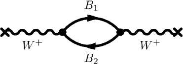
Figure 21: The one-loop polarization tensor for charged current process. The wavy lines correspond to the $W^{+}$ propagators, the solid line to the baryonic propagators.

3.3.1 One-loop processes

The one-loop polarization tensor is shown in Fig. 21; the corresponding analytical expression is

$$i\Pi_{\mu\nu}^{<}(q)=\int\frac{d^{4}p}{(2\pi)^{4}}\frac{d^{4}p^{\prime}}{(2\pi)^{4}}{\rm Tr}\left[\Gamma_{\mu}G^{<}(p)\Gamma_{\nu}G^{>}(p^{\prime})\right](2\pi)^{4}\delta^{4}(q+p^{\prime}-p)=T_{\mu\nu}{\cal L}(q),$$ (219)

where the charged current weak interaction vertices are $\Gamma_{\mu}=\tilde{G}_{F}\gamma_{\mu}(1-g_{A}\gamma^{5})$ with $g_{A}=1.26$ being the axial coupling constant, the tensor $T_{\mu\nu}=-\tilde{G}^{2}g_{x}^{2}$ where $g_{X}=1$ for $\mu=\nu=0$ and $g_{X}=g_{A}$ for $\mu=\nu=1,2,3$; the loop integral can be computed analytically in the quasiparticle limit

$${\cal L}(\bm{q},\omega) = \frac{m^{*}_{B}m^{*}_{B^{\prime}}}{2\pi\beta|q|}{\rm ln}\Bigg{|}\frac{1+{\rm exp}\left[-\beta\left(\xi-\mu_{B}\right)\right]}{1+{\rm exp}\left[-\beta\left(\xi-\mu_{B}\right)-\beta\omega\right]}\Bigg{|}\equiv\frac{m^{*}_{B}m^{*}_{B^{\prime}}}{2\pi\beta|q|}L(\omega,q),$$ (220)

where $m^{*}_{B}$ is the effective mass of a quasiparticle of baryon type $B$, $\xi=\tilde{p}^{2}/2m-\mu_{B}$ and $\tilde{p}=(m^{*}_{B}/q)(\omega-\mu_{B}+\mu_{B^{\prime}}-q^{2}/2m^{*}_{B})$, where we assume that $m^{*}_{B}\simeq m^{*}_{B^{\prime}}$. This result can be substituted in Eq. (218) to obtain, for example, the emissivity of the Urca process $n\to p+e+\bar{\nu}$ [200]

$$\epsilon_{\bar{\nu}} = \epsilon_{0}\int_{-\infty}^{\infty}dy~{}g(y)~{}L(y,p_{Fe})\int_{0}^{\infty}dzz^{3}f_{e}(z-y),\quad\epsilon_{0}=(1+3g_{A}^{2})\frac{3\tilde{G}^{2}m_{n}^{*}m_{p}^{*}p_{Fe}}{2\pi^{5}\beta^{6}},$$ (221)

where $p_{Fe}$ and $f_{e}$ are the Fermi-momentum and distribution function of electrons and $y=\beta\omega$. In the zero temperature limit $L(y,p_{Fe})=y\theta(-\beta\xi)$, the integrals in Eq. (221) can be performed analytically and one recovers the zero-temperature result of Lattimer et al. [189]. The zero temperature $\theta$-function can be rewritten as $\theta(p_{Fe}+p_{Fp}-p_{Fn})$ [189] which tells us that the “triangle inequality” $p_{Fe}+p_{Fp}\geq p_{Fn}$ must be obeyed by the Fermi-momenta of the particles for the Urca process to operate.

The emissivity of the Urca processes (221) scales as $\tilde{G}^{2}$, since the process is second order in the weak interactions; its linear dependence on the effective masses of participating baryons arises through their density of states $\nu\sim m^{*}p_{F}/\pi^{2}$, where $p_{F}$ stands for the Fermi momentum; the density of states of massless electrons contributes the factor $p_{Fe}^{2}$ and a factor $1/p_{Fe}$ arises from the momentum conservation condition. The temperature dependence can be understood from the dimensional analysis of the reaction rate and arises as follows [190]: each degenerate fermion being confined to a narrow band $\sim T$ around the Fermi surface contributes a factor $T$, the final state anti-neutrino contributes a factor $T^{3}$; an additional factor $T$ is due to the fact that we are interested in the energy rate and a compensating factor of $1/T$ arises due to the energy conservation constraint.

Eq. (221) can be adapted to describe the Urca processes (191) which involve hyperons [194]. Among these the process $\Lambda^{0}\to p+e^{-}+\bar{\nu}$ is potentially important. The corresponding triangle inequality follows from the theta function $\theta(p_{Fe}+p_{Fp}-p_{F\Lambda})$. Since typically $p_{Fe}\sim p_{Fp}\ll p_{Fn}$ a small fraction of $\Lambda$’s is sufficient for the reaction to operate. Although it is less effective than the nucleonic Urca process, since it involves a change of strangeness and its matrix element is proportional to ${\rm sin~{}}^{2}\theta_{C}$, it is still as efficient as other exotic cooling channels e.g. the pion decay (194) or kaon decay (195).

For identical baryons the one-body bremsstrahlung process (186) vanishes, as can be seen from Eq. (220) in the limit of equal chemical potentials (note that in the non-relativistic kinematics spurious terms remain, which vanish exactly if the proper relativistic kinematics is used). However there are cases where the one-loop bremsstrahlung is possible because the baryons are embedded in a mean-field; an example are the CPBF processes which arise due to the pairing mean field (see subsection 3.5). Yet another possibility arises when the baryons are coupled to external gauge fields. Canonical neutron stars support magnetic fields, of the order of $10^{12}-10^{13}$ G. A separate class of neutron stars, know as magnetars, are believed to support fields that are much larger, of the order of $B\sim 10^{15}-10^{17}$ G [203]. The interaction of the baryon magnetic moment with the applied field induces a splitting in the energy of spin-up and spin-down baryons of the order of $\mu^{(B)}B$, where $B$ is the magnetic induction, $\mu^{(B)}$ is the fermion magnetic moment. For neutrons $\mu^{(n)}=g_{n}\mu_{N}$, where the gyromagnetic ratio $g_{n}=-1.913$; for protons $\mu^{(p)}=g_{p}\mu_{N}$, $g_{p}=2.793$, where $\mu_{N}=e\hbar/2m_{p}=3.152\times 10^{-18}$ G^-1 MeV is the nuclear magneton. Thus, we can expect non-vanishing neutrino bremsstrahlung as a result of the Pauli spin-paramagnetic splitting whenever the $2\mu^{(B)}B\sim T$ [204]. For neutrons the Pauli paramagnetism is the only effect that affects the quasiparticle spectrum, which is written as (to the leading order in $B^{2}/m_{N}$)

$$\varepsilon_{n}(s)=(m_{n}^{2}+p^{2}-2sm_{n}\mu^{(n)}B)^{1/2},$$ (222)

where the spin projections on the magnetic axis are $s=\pm 1$. The quasiparticle spectrum of charged particles includes in addition to the Zeeman splitting the Landau quantization of orbits in the plane transverse to the direction of the applied field

$$\varepsilon_{pN}(s)=[m^{2}+p^{2}_{z}+(2N+1-sg_{p})eB]^{1/2},$$ (223)

where $N$ labels the Landau levels. The emissivity due to the $n\to n+\nu+\bar{\nu}$ process is obtained as [204]

$$\epsilon_{\nu\overline{\nu}}=\frac{G_{F}^{2}c^{2}_{A}m_{N}^{2}}{2(2\pi)^{5}}T^{7}\int_{0}^{\infty}dy\frac{y^{4}}{e^{y}-1}\int_{0}^{y}dx\Bigg{(}\ln\frac{e^{-\beta E_{-}}+1}{e^{-\beta E_{-}-y}+1}-\ln\frac{e^{-\beta E_{+}}+1}{e^{-\beta E_{+}-y}+1}\Bigg{)},$$ (224)

where $E_{\pm}=(m_{N}^{2}+p^{2}_{\pm}-sg_{n}eB)^{1/2}$ and $p_{\pm}$ are the upper and lower bounds on the momenta imposed by the integration over the angle between the particle momentum and the momentum transfer in the process.

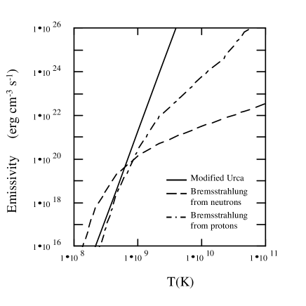
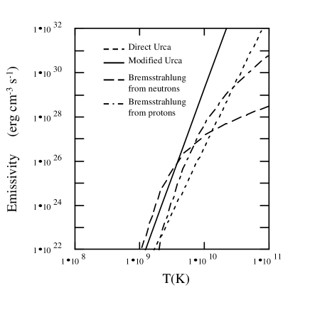
Figure 22: The emissivities of various processes vs the temperature for fields $B=10^{16}$ (left panel) and $B=10^{17}$ G (right panel).

The emissivity involves only axial currents because the process requires a spin-flip whereby a quasiparticle is transfered from one Fermi surface (of the spin-up population) to the other surface (spin-down population). The dependence on the effective masses arises from the phase space integration which introduces a density of states per particle. The analysis of the temperature dependence is similar to the case of the Urca process, with the only difference that the transfered momentum is of the order of $T$ (rather than $p_{Fe}$) therefore an additional factor $T$ appears. Note that this bremsstrahlung process vanishes in the zero field limit. Several authors considered the Urca process in strong magnetic fields, where the effects of Landau quantization change the qualitative picture by removing the “triangle inequality” constraint [204, 205, 206].

The temperature region where the one-body neutrino-pair bremsstrahlung is important increases with increasing magnetic field (see Fig. 22). The pair bremsstrahlung from neutrons is efficient whenever $|\mu_{n}|B\sim T$, since then the energy involved in the spin-flip is of the same order of magnitude as the thermal smearing of the Fermi surface. The temperature at which neutrino-pair bremsstrahlung from neutrons becomes comparable to the competing processes roughly coincides with this condition. For lower temperatures the emissivity drops exponentially, because the energy transfer becomes larger than the thermal smearing. Neutrino-pair bremsstrahlung from protons is important when $\mu_{p}B\sim T$. The emissivity due to the protons increases faster than the emissivity due to the neutrons with the temperature, since the smearing of the proton transverse momenta provides an additional relaxation on the kinematical constrains. According to Fig. 22 the emissivity of the modified Urca process is larger than that of neutrino-pair bremsstrahlung from neutrons and protons at high temperatures, mainly due to the different temperature dependencies of these processes ($\propto T^{7}$ for the one-body bremsstrahlung as compared to $\propto T^{8}$ for the modified Urca). However, for temperatures that are smaller than $\mu_{p}B\sim T$ the emissivity drops just as for neutrons - exponentially. In the case of a superstrong magnetic field $B\geq 10^{17}$ G the large uncertainty in the transverse momenta of the protons and electrons allows the direct Urca process to occur, and its emissivity dominates the emissivity of any other process.

3.3.2 Two-loop processes

The nuclear interaction enters the quasiparticle loop expansion at the second order. To compute the emissivity we need a model of nuclear scattering in background medium. The form of the nuclear interaction depends, of course, on the nuclear matter model one works with. Below we will give a specific example of the computation of the neutral current bremsstrahlung process $n+n\to n+n+\nu+\bar{\nu}$ [202]. The effective particle-hole interaction can be represented by pion-exchange at long distances and contact Fermi-liquid interaction at short distances [207]

$$V_{[ph]}(k)=\left(\frac{f_{\pi}}{m_{\pi}}\right)^{2}\left(\bm{\sigma}_{1}\cdot\bm{k}\right)D^{c}(\bm{k})\left(\bm{\sigma}_{2}\cdot\bm{k}\right)+f_{0}+f_{1}(\bm{\sigma}_{1}\cdot\bm{\sigma}_{2}),$$ (225)

where $f_{\pi}$ is the pion decay constant, $m_{\pi}$ is the pion mass, $D^{c}(\bm{k})$ is the on-shell causal pion propagator, $f_{0}$ and $f_{1}$ are the coupling parameters of the Fermi-liquid theory, $\bm{\sigma}$ is the vector of the Pauli matrices. The form of the $ph$ interaction is suitable when the scales in the problem can be separated with respect to the Compton length of the pion $\lambda_{\pi}=m_{\pi}^{-1}=1.4$ fm. If the system is characterized by scales $L\gg\lambda_{\pi}$ (e.g. is sufficiently dilute) the only relevant dynamical degree of freedom is pion and the rest of the nuclear interaction can be approximated by constants. To obtain values of neutrino emissivities that are consistent with those computed from the nuclear $T$-matrix the $\rho$ meson exchange needs to be included explicitly in Eq. (225).

The topologically non-equivalent two-loop diagrams of our theory are shown in Fig. 23.

Figure 23: The two-loop polarization tensor. The wavy lines correspond to the $W^{+}$ propagators, the solid lines to the baryonic propagators, the dashed lines to nuclear interactions.

The analytical expression, corresponding to the first (from left to right) diagram in Fig. 23, is

$$i\Pi^{<,\,a}_{\mu\nu}(q) = \int\!\!\prod_{i=1}^{4}\left[\frac{d^{4}p_{i}}{(2\pi)^{4}}\right]\frac{dk}{(2\pi)^{4}}(2\pi)^{8}\delta(q+p_{4}-k-p_{3})\delta(k+p_{2}-p_{1}){\rm Tr}\left[V(k)G^{<}(p_{1})V(k)G^{>}(p_{2})\right]$$ (226)

$${\rm Tr}\Bigl{[}\Gamma_{\mu}G^{c}(q+p_{4})V(k)D^{c}(k)G^{<}(p_{3})V(k)D^{a}(k)G^{a}(q+p_{4})\Gamma_{\nu}G^{>}(p_{4})\Bigr{]},$$

where $V(k)$ is the strong interaction vertex, which can be read-off from Eq. (225). The contribution of this diagram is readily recognized as a propagator dressing in the $ph$ channel by a self-energy which involves an excitation of particle-hole collective mode. The second diagram in Fig. 23 corresponds to a vertex correction in the $ph$ channel by an effective interaction, which incorporates an intermediate the particle-hole collective mode excitation. The third diagram in Fig. 23 may be interpreted as a particle-hole fluctuation. These diagrams for model interaction (225) show the following features: (i) the vector current contributions from the first and second diagrams mutually cancel; (ii) the third diagram does not contribute because the axial-vector contribution involves traces over odd number of $\sigma$-matrices and the vector-current contribution is canceled by an equal and of opposite sign contribution from the diagram which is generated from the third diagram by flipping one of the loops upside-down; (iii) all contributions due to the Fermi-liquid interaction cancel after summing the first two diagrams. Note that the exchange diagrams are generated from the direct ones by means of interchanging the outgoing propagators in a strong vertex.

The causal propagator in Eq. (226) have the following general equilibrium form

$$G^{c}(p)=\frac{\omega-(\varepsilon_{p}-\mu)}{\left[\omega-(\varepsilon_{p}-\mu)\right]^{2}+\gamma^{2}(p)/4}-\frac{i\gamma(p)/2}{\left[\omega-(\varepsilon_{p}-\mu)\right]^{2}+\gamma^{2}(p)/4}{\rm tanh}\left(\frac{\beta\omega}{2}\right),$$ (227)

where ${\rm tanh}\left({\omega}/{2}\right)\equiv[1-2f_{F}(\omega)]$ and $\epsilon_{p}=p^{2}/2m+\mathop{\rm Re}\Sigma(p)$. The arguments of the causal propagators in the diagrams in Fig. 23 contain the external four momentum $q$ and the propagation between the strong and weak vertex it describes is off the mass-shell. The off-shell dependence of the propagator can be simplified by expanding with respect to small parameter $v\ll 1$ which is the characteristic velocity of a baryon (the velocity of light $c=1$ and we use non-relativistic kinematics)

$$(\omega+\varepsilon_{p})-\varepsilon_{\vec{p}+\vec{q}}\simeq\omega-\bm{p}\cdot\bm{q}/m-q\frac{\partial}{\partial p}~{}\mathop{\rm Re}\Sigma(p)-\epsilon_{q}\simeq\omega,$$ (228)

to the leading order. For off-shell energies not far from the Fermi energy the quasiparticle damping is an even function of the frequency $\gamma(-\omega)=\gamma(\omega)$ (this observation is exact in the phenomenological Fermi-liquid theory and is confirmed by microscopic calculations). Then

$$G^{c}(\pm\omega,\bm{p}) = \pm\frac{\omega}{\omega^{2}+\gamma(\omega,\bm{p})^{2}/4}\mp i\frac{\gamma(\omega,\bm{p})/2}{\omega^{2}+\gamma(\omega,\bm{p})^{2}/4}~{}{\rm tanh}\left(\frac{\beta\omega}{2}\right).$$ (229)

Note that the acausal propagator is obtained from the above through complex conjugation $[G^{c}(p)]^{*}=-G^{a}(p)$. We conclude that the propagator (229) is odd under the exchange of the sign of $\omega$, a property which is important for the vector current conservation. We now write down the neutrino emissivity for the $n+n\to n+n+\nu+\bar{\nu}$ process which is the sum of diagrams in Fig. 23

$$\epsilon_{\nu\bar{\nu}} = \frac{32}{5(2\pi)^{9}}G_{F}^{2}g_{A}^{2}\left(\frac{f_{\pi}}{m_{\pi}}\right)^{4}\,\left(\frac{m^{*}}{m}\right)^{4}\,p_{F}\,I\,T^{8}=5.5\times 10^{19}\,I_{3}\,T_{9}^{8}~{}({\rm erg~{}cm^{-3}~{}s^{-1}})$$ (230)

where $T_{9}$ is the temperature in units of $10^{9}$ K, $I_{3}$ is the integral $I$ in units $10^{3}$ defined as

$$I = \int_{0}^{\infty}dy\,y^{6}|G^{c}(y)|^{2}{\cal Q}(y)\int^{\infty}_{0}dxx^{4}|D^{c}(x)|^{2}\int_{-\infty}^{\infty}dz~{}g(z)~{}g(y-z){L}(z,x){L}(y-z,x).$$ (231)

The temperature dependence in Eq. (230) can be understood by comparing the modified processes to their one-body counterparts discussed above. The additional fermion appearing in the initial and final state introduces an additional factor $(T/E_{F})^{2}$. Since this argument applies equally well to the modified Urca process, we conclude that its emissivity scales with temperature as $T^{8}$. The scaling of emissivity with the effective mass arises due to its dependence on the density of states of the initial and final baryons. Each strong interaction vertex introduces a power of the pion-nucleon coupling, therefore $\epsilon_{\nu\bar{\nu}}\propto f_{\pi}^{4}$ (see Fig. 23). The simplest approximation to the pion propagator in Eq. (231) is to neglect the pion self-energy and approximate it as $D^{c}(k)=[\bm{k}^{2}+m_{\pi}^{2}]^{-1}.$ The free-space approximation should be valid in the vicinity of the nuclear saturation density and below. The softening of the one-pion exchange (a precursor of the pion-condensation) increases the neutrino emissivity by large factors, see for details ref. [201]. The Pauli blocking of the final state neutrino at finite temperatures is taken into account by the function ${\cal Q}(y)$; In the dilute (anti-)neutrino limit $\beta\mu_{\nu_{f}}\ll 1$ (where $\mu_{\nu_{f}}$ is the chemical potential of neutrinos of flavor $f$) ${\cal Q}(y)=1$. This is the case below the temperatures where the neutrinos are trapped. In the low-temperature limit ${\cal L}(z)=z$ and the $z$-integration decouples from the $x$-integration. Letting $\gamma(\omega)\to 0$ (quasiparticle limit) one finds that $G^{c}(\omega)=\omega^{-2}$. Then, the $z$ integration can be carried out analytically upon dropping the wave-function renormalization contribution:

$$\int_{-\infty}^{\infty}\!\!dz~{}g(z)\,g(y-z)~{}z~{}(y-z)=\frac{y~{}(y^{2}+4\pi^{2})}{6~{}(e^{y}-1)}.$$ (232)

After these manipulations Eq. (230) reduces to the quasiparticle result of ref. [207]. It should be noted here that the OPE approximation to the nucleon-nucleon amplitude is not justified in dense matter from the numerical point of view, and one should include other mesons to take into account for the intermediate range attraction and short-range repulsion. In particular the inclusion of the $\rho$ meson repulsion modifies the meson propagator to [208] $D^{c}(k)=[\bm{k}^{2}+m_{\pi}^{2}]^{-1}-C_{\rho}[\bm{k}^{2}+m_{\rho}^{2}]^{-1},$ where $C_{\rho}=1.67$ and $m_{\rho}\simeq 600$ MeV. Such a correction substantially improves upon the OPE result and a quantitative agreement is achieved between the $\pi\rho$-exchange model and full $T$-matrix calculations [209] or low-momentum interactions [210].

3.3.3 Landau-Pomeranchuck-Migdal effect

In this subsection we explore the effect of the finite width in the causal propagator (229) which describes the off-shell propagation between the weak and strong vertices. The off-shell propagations is characterized by a length (or time) scale known as the formation length (time) first introduced in the context of bremsstrahlung of charge particles passing through matter by Ter-Mikaelian [211, 212]. In our context the gauge boson energy is soft $\omega\ll E_{F}$ and can be associated with the formation length

$$l_{f}=\frac{\hbar}{\omega}v_{F}=\tau_{f}v_{F},$$ (233)

where $v_{F}$ is the baryon Fermi-velocity. The formation length is the distance that a particle covers during the emission of the gauge boson; if $v_{F}$ is large and $\omega$ small, $l_{f}$ can be very long. This observation was the basis for the suppression calculation by Landau and Pomeranchuk [213] and Migdal [214] in the context of high-energy electrons radiating photons.

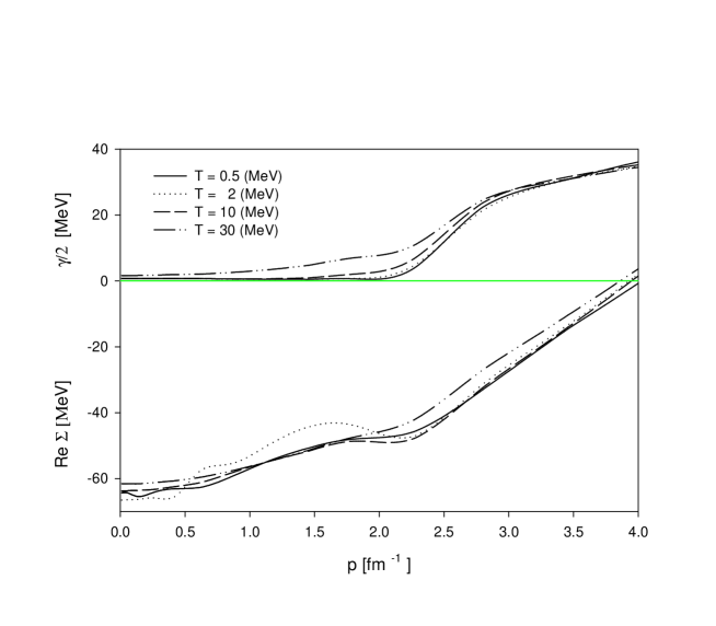
Figure 24: The on mass-shell damping $\gamma$ (upper panel) and the real part of the self-energy (lower panel) as a function of the particle momentum for neutron matter at density $\rho_{0}=0.16$ fm^-3.

There is another scale in the problem - the mean-free-path of a quasiparticle,

$$l_{mfp}=\tau_{mfp}v_{F}=(n\sigma)^{-1}\left(\frac{E_{F}}{T}\right)^{2}v_{F},$$ (234)

where $\sigma\sim 40$ mb is the baryon-baryon cross-section (mb $=10^{-26}$ cm²), $n$ is the baryon number density. In the limit $l_{mfp}\gg l_{f}$ the radiation is from a well defined source - the environment has no influence on the radiation. In the opposite limit $l_{mfp}\ll l_{f}$, the baryon-baryon interaction need to be included in the renormalized propagators, which are now the fundamental degrees of freedom to treat the radiation process. In the case where $l_{mfp}\sim l_{f}$ the radiation is suppressed since the baryon-baryon collisions interfere (destructively) with the emission process.

In our context the Landau-Pomeranchuk-Migdal (LPM) effect is described by the finite width of the quasiparticles in Eq. (229). The finite width not only suppresses the radiation, but also regularizes the infrared divergence of the radiation cross-section; in the case of the neutrino-bremsstrahlung processes this divergences is absent even in the zero width limit because of high powers of $\omega$ appearing in the numerator of the emissivity.

The width of the quasiparticle propagators can be parameterized in terms of the reciprocal of the quasiparticle life time in the Fermi-liquid theory:

$$\gamma=aT^{2}\left[1+\left(\frac{\omega}{2\pi T}\right)^{2}\right],$$ (235)

where $a$ is a density dependent phenomenological parameter. Fig. 24 illustrates the real part of the self-energy and the damping in neutron matter computed within the finite temperature version of the BBG theory. In this version of the theory the $K$ matrix is complex valued [202].

The emergent neutrino spectrum can be characterized by the spectral function

$$S(y) = |G^{c}(y)|^{2}{\cal Q}(y)\int^{1}_{0}dxx^{4}|D^{c}(x)|^{2}\int_{-\infty}^{\infty}dz~{}g(z)~{}g(y-z){L}(z,x){L}(y-z,x).$$ (236)

The dependence of the integral on the (dimensionless) neutrino frequency $y=\beta\omega$ at $T=20$ MeV and the saturation density $\rho_{0}$ is shown in Fig. 25 for three cases: the limit of vanishing width (dashed line), including the leading order in $\gamma$ contribution in the width [i. e. the first term in Eq. (229)] (dashed-dotted line) and the full non-perturbative result (solid line). The energy carried by neutrinos is of order of $\omega\sim 6T$ in all three cases since the average energy carried by each neutrino (non-interacting relativistic massless particle) is $3T$. The finite width of propagators leads to a suppression of the bremsstrahlung rate. Keeping the full non-perturbative expression for the causal propagators enhances the value of the integral with respect to the leading order perturbative result. The LPM effect sets in when $\omega\sim\gamma$. As neutrinos are produced thermally, the onset temperature of the LPM effect is of the order of $\gamma$. Equation (235) shows that the value of the parameter $a$ controls the onset temperature which turns out to be of the order of 5 MeV.

Figure 25: The neutrino spectral function (236) at the temperature $T=20$ MeV and density $\rho_{0}=0.16$ fm^-3. The dashed curve is the zero width limit, the dashed-dotted curve includes only the leading order in $\gamma$ contribution from the causal propagator, the solid curve is the full non-perturbative result.

An alternative to the two-loop calculation outlined above is the computation based on a one-loop polarization tensor with fully off-shell propagators, as suggested in the case of photoemission in ref. [215] and neutrino emission in ref. [191]. However, dressed propagators need to be supplemented with dress vertex functions that satisfy the Ward identities in self-consistent manner; the problem of dressed vertices is discussed in ref. [216]. Multi-pair excitations processes, that are relevant to the description of the LPM effect within the Landau-Fermi liquid theory are discussed in Refs. [217, 218].

3.3.4 Soft-neutrino approximation

The soft neutrino approximation arises in the models that are based on either the free-space or medium modified $T$-matrix theories [219, 220, 221]. We have seen that the typical energy carried by neutrinos is of the order of several MeV, which is small on the nuclear energy scales of tens of MeV. The neutrino bremsstrahlung process is therefore called “soft”. Note that this is not the case for the Urca processes, where the electron energy is of the same order of magnitude as the neutron energy. In the case of the bremsstrahlung one can apply the ideas underlying the Low theorem for the photon bremsstrahlung which states that the bremsstrahlung amplitude to the leading $O(\chi^{-1})$ and next-to-leading $O(1)$ order in the expansion with respect to $\chi=\omega/E_{f}$, where $\omega$ and $E_{F}$ are the characteristic energies of neutrinos and baryons, is determined by the non-radiative cross-section. The weak matrix element is written as

$${\cal M}_{\mu}^{a}=T(p_{1}\,p_{2}^{\prime};p_{1}-q,p_{2})G(p_{1}-q)\Gamma_{\mu}+\gamma_{\mu}G(p_{1}^{\prime}+q)T^{\prime}(p_{1}^{\prime}+q,p_{2}^{\prime};p_{1},p_{2})+(1\leftrightarrow 2),$$ (237)

where $T$ is the scattering $T$-matrix, $G(p)=m\Lambda^{+}/(p\cdot q)$ is the free-space Green’s function with the positive energy projector defined as $\Lambda^{+}(p)=(\!\not\!p+m)/(2m)$, $\Gamma_{\mu}=(G_{F}/\sqrt{2})\gamma_{\nu}(c_{V}-c_{A})(\tau_{a}/2)$ is the weak interaction vertex and $\tau^{a}$ is the isospin operator. Next, expand the $T$-matrices in (237) around their on-shell matrix $T_{0}$

$$T_{1}=T_{0}-q\cdot\partial_{p_{1}}T_{0}+\dots\quad T_{1}^{\prime}=T_{0}-q\cdot\partial_{p_{1}^{\prime}}T_{0}+\dots$$ (238)

The expansion of Eq. (237) can be divided into the external and internal contributions, depending whether the neutrino is emitted from the external leg of the $T$-matrix or from the internal interaction line (see Fig. 26). For the vector current the external term can be computed explicitly while the form of the internal term is fixed from the requirement of the vector current conservation $q^{\mu}{\cal M}_{\mu}^{V,a}=0$. For the axial vector case one needs to take into account the concept of partially conserved axial currents (PCAC) which leads to the condition [219]

$$q^{\mu}{\cal M}_{\mu}^{A,a}=\frac{f_{\pi}}{2}\frac{m_{\pi}^{2}}{q^{2}+m_{\pi}^{2}}{\cal M}_{\pi}^{a},$$ (239)

where ${\cal M}_{\pi}^{a}$ is the pion emission matrix element.

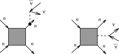
Figure 26: Illustration of the external (left graph) and internal (right graph) contributions to the neutrino bremsstrahlung. The shaded block corresponds to the $T$-matrix, the dashed line to the weak interaction, the arrows to the participating particles.

To the leading order in the expansion with respect to the small parameter $\chi$, i. e. $O(\chi^{-1})$ the vector and axial vector matrix elements read

$${\cal M}_{\mu}^{V,a} = \frac{G_{F}c_{V}}{2\sqrt{2}}\left(-T_{0}\frac{p_{1\mu}}{p_{1}\cdot q}\tau^{a}+\tau^{a}\frac{p^{\prime}_{1\mu}}{p_{1}^{\prime}\cdot q}T_{0}\right)+\{1\leftrightarrow 2\},$$ (240)

$${\cal M}_{\mu}^{A,a} = \frac{mG_{F}c_{V}}{\sqrt{2}}\left(-T_{0}\frac{\Lambda^{+}(p_{1})}{p_{1}\cdot q}\gamma_{\mu}\gamma_{5}\tau^{a}+\gamma_{\mu}\gamma_{5}\tau^{a}\frac{\Lambda^{+}(p^{\prime}_{1})}{p_{1}^{\prime}\cdot q}T_{0}\right)+\{1\leftrightarrow 2\}.$$ (241)

It can be verified that the vector current is conserved. For matrix elements with the nucleons on the mass shell, the most general nonrelativistic charge-independent nucleon-nucleon amplitude contains central, spin-spin, tensor, spin-orbit, and quadratic spin-orbit terms. For fixed isospin it can be written

$$T=T_{C}+T_{S}\bm{\sigma}_{1}\cdot\bm{\sigma}_{2}+T_{T}S_{12}+T_{SO}{\bm{L}}\cdot{\bm{S}}+T_{Q}Q_{12}$$ (242)

where the tensor and quadratic spin-orbit operators are defined as $S_{12}=3{\bm{\sigma}_{1}\cdot\bm{r}}{\bm{\sigma}_{2}\cdot\bm{r}}-\bm{\sigma}_{1}\cdot\bm{\sigma}_{2}$ and $Q_{12}=({\bm{\sigma}_{1}\cdot\bm{L}}{\bm{\sigma}_{2}\cdot\bm{L}}+{\bm{\sigma}_{2}\cdot\bm{L}}{\bm{\sigma}_{1}\cdot\bm{L}})/2$.

Consider the process $n+n\to n+n+\nu+\bar{\nu}$. In the non-relativistic limit $p\cdot q=\bm{p}\cdot\bm{q}-m\omega\simeq m\omega$ to leading order in $v_{F}/c$ and the vector current contribution (240) vanishes. The contribution from the axial-vector current is given by the commutator

$${\cal M}_{0}^{A}=0,\quad{\bm{M}}^{A}=\frac{G_{F}}{2\sqrt{2}}\frac{g_{A}}{\omega}[T^{nn},{\bm{S}}],$$ (243)

where ${\bm{S}}=(\bm{\sigma}_{1}+\bm{\sigma}_{2})/2$, ${\bm{M}}^{A}$ is the spatial component of the vector ${\cal M}^{A}_{\mu}$, $T^{nn}$ is the neutron-neutron scattering $T$-matrix and the axial coupling constant $g_{A}=1.26$. The commutator (243) is non-zero only for the tensor, spin-orbit and quadratic spin-orbit terms in the expansion (242), therefore only spin-triplet nucleon-nucleon partial waves contribute. The dominant tensor force is much stronger in the $np$ system and despite the fact that the proton fraction is small the process $n+p\to n+p+\nu+\bar{\nu}$ can gain significance. The vector and axial-vector matrix elements of this process in the non-relativistic and soft-neutrino approximations are

$${\cal M}^{V}_{0}=-\frac{\bm{q}}{\omega}\cdot{\bm{M}}^{V},\quad{\bm{M}}^{V}=-\frac{G_{F}}{2\sqrt{2}}\frac{c_{V}^{n}-c_{V}^{p}}{\omega}\frac{\bm{k}}{m}T^{np},$$ (244)

$${\cal M}^{A}_{0}=0,\quad{\bm{M}}^{A}=\frac{G_{F}}{\sqrt{2}}\frac{g_{A}}{\omega}[T^{np},{\bm{S}}^{-}],$$ (245)

where $\bm{k}=\bm{p}-\bm{p}^{\prime}$, ${\bm{S}}^{-}=(\bm{\sigma}_{1}-\bm{\sigma}_{2})/2$, $c_{V}^{n}=-1$, $c_{V}^{p}=1-4{\rm Sin}^{2}\theta_{W}$. The soft neutrino approximation is not valid for the modified Urca process (187) as the energy transfer in the reaction could be large, of the order of the neutron Fermi-energy. The neutrino emissivities evaluated with the matrix elements quoted above (which thus include the full $T$-matrix) are reduced by factor 4-5 compared to the results obtained with the one-pion-exchange amplitudes [219, 220, 221, 209], but are of the same magnitude if the OPE is supplemented by repulsive $\rho$-meson exchange.

3.4 Graviton emission in Kaluza-Klein theories

We have seen that the charged current two-loop process - the modified Urca reaction - is dominant among these type of reactions. There is a distinct physical situation where only the charge-neutral current processes contribute - the case of gravitational bremsstrahlung [221, 222]. This process arises within the models where the standard model fields live on a four-dimensional manifold, while gravity is allowed to propagate in ($n+4$) dimensions, where $n$ is the number of extra dimensions. Such schemes provide a natural explanation of the hierarchy problem in particle physics; the gravity appears to be much weaker that the remaining three fundamental forces because it is diluted by its extension in extra dimensions. This picture fits into the traditional Kaluza-Klein (KK) theories which contain the usual four dimensional space-time manifold plus additional compact dimensions which form an unobservable, small manifold (which until recently was believed to be Planck size $\sim M_{P}^{-1}$, where $M_{P}=1.2\times 10^{19}$ GeV). Recent models of extra dimensional gravity propose that there are $n$ extra compact dimensions, all of which are about the same size $R$ and $R$ is much larger than the Planck scale, possibly as large as a millimeter [223, 224]. The size $R$ of the extra dimensions is given in terms of the Planck mass $M_{P}$ and an effective mass $M$, which is taken of the order of 1 TeV, as

$$R^{n}\sim\frac{M_{P}^{2}}{M^{n+2}}.$$ (246)

At scales of the order of $R$ the Newtonian gravity is expected to fail. If $n=1$ then for $M\sim 1$ TeV one finds $R\sim 10^{10}$ km, which implies that there must be deviations from Newtonian gravity over solar system distances. However, if $n=2$ then $R\leq 1$ mm. Since gravity has not been tested at distances smaller than millimeter, large extra dimensions are consistent with present experimental knowledge. An interesting consequence of this theory is that a $4+n$ dimensional graviton can propagate in extra dimensional space, while the standard model particles are confined to the four dimensional space.

The size of the extra dimensions can be constrained if there is an evidence of missing energy in astrophysical processes such as supernova explosions. Since the models of supernovae based on the standard physics explain the duration and energy of the neutrino pulse observed from SN1987A, any mechanism that drains sufficient energy from the core of the supernova will destroy the agreement. The bremsstrahlung of gravitons in the nucleon-nucleon collision was suggested as such a mechanism [223]. The interaction between gravitons and dilatons and the standard model particles is described by the Lagrangian density

$${\cal L}=-\frac{\kappa}{2}\sum_{\vec{j}}\left[h^{\mu\nu,\bm{j}}T_{\mu\nu}+\left(\frac{2}{3(2+n)}\right)^{1/2}\phi^{\bm{j}}T_{\mu}^{\nu}\right],$$ (247)

where $h^{\mu\nu,\bm{j}}$ and $\phi^{\bm{j}}$ are the graviton and dilaton fields, $\bm{j}$ is an $n$-dimensional vector representing the momentum of the mode in the extra dimensions. The differential rate at which the KK particles escape into extra dimensions can be related to the on-shell $T$-matrix in neutron matter and is given by the expression [221]

$$\frac{d\epsilon_{KK}}{d\omega}=\frac{8G_{N}}{5\pi}\frac{k}{\omega}\left(\frac{4\overline{p^{2}}}{m_{N}}\right)^{2}{\rm sin~{}}^{2}\theta_{cm}|T|^{2}\left\{\begin{array}[]{cc}{2}\left(1-\gamma_{\bm{j}}\right)^{2}/[9(2+n)]\\ {19}/{18}+{11}\gamma_{\bm{j}}^{2}/9+2\gamma_{\bm{j}}^{4}/9\end{array}\right.,$$ (248)

where the upper line corresponds to extra-dimensional gravitons, the lower line to dilatons, $\gamma_{\bm{j}}\equiv m_{\bm{j}}^{2}/{\omega^{2}}$ and $m_{\bm{j}}=\bm{j}^{2}/R^{2}$ is the effective mass of KK particles on the four dimensional brane; here $G_{N}$ is Newton’s constant, $\overline{p^{2}}=p^{{}^{\prime}2}+p^{2}$ and ${\rm cos~{}}\theta_{cm}=\hat{p}\cdot\hat{p}^{\prime}$, where $\bm{p}$ and $\bm{p}^{\prime}$ are the momenta of colliding neutrons, $k$ and $\omega$ are the momentum and energy of radiated particles. The gravitational emissivity is obtained upon taking the phase-space integrals over the rates (248) and summation over the momenta $\bm{j}$. The bounds obtained with the one-pion-exchange approximation and the full $T$-matrix (and an analog of the soft neutrino approximation) are

$$R<\left\{\begin{array}[]{ll}7\times 10^{-4}{\rm mm}\quad(n=2),&9\times 10^{-7}{\rm mm}\quad(n=3),\\ 3\times 10^{-4}{\rm mm}\quad(n=2),&4\times 10^{-7}{\rm mm}\quad(n=3),\end{array}\right.$$ (249)

where the upper and lower lines differ mainly in the treatment of the nuclear interaction: the upper line corresponds to the free space interaction between nucleon in terms of a $T$-matrix [221], the lower line to the one-pion-exchange [222] interaction. These bounds provide one of the most important constraints on the size of extra dimensions, assuming that our current understanding of the supernova mechanism and energetics is correct.

3.5 The role of pairing correlations in neutrino radiation rates

Pairing correlations play a twofold role in the thermal evolution of neutron stars. At asymptotically low temperatures they suppress the neutrino emission processes exponentially, because the number of excitations vanishes as exp$(-\Delta/T)$, where $\Delta$ is the gap in the quasiparticle spectrum. At moderate temperatures $T\leq T_{c}$ the pairing field lifts the constraints on the one-body (quasiparticle) bremsstrahlung (186) and opens a new channel of neutrino radiation [197, 198]. The corresponding charge-neutral current diagrams are shown in Fig. 27. These diagrams are associated with the following polarization tensor

$$i\Pi_{V/A}^{<}(q)=-2g_{B}(q_{0})\mathop{\rm Im}\Pi_{V/A}(q)=\sum_{\sigma}\int\frac{d^{4}p}{(2\pi)^{4}}\left[G^{<}(p+q)G^{>}(p)\mp F^{<}(p+q)F^{>\dagger}(p)\right],$$ (250)

where $G(p)$ and $F(p)$ are the normal and anomalous propagators, defined in Subsec. 2.2.2, the $\sigma$-summation is over the spins.

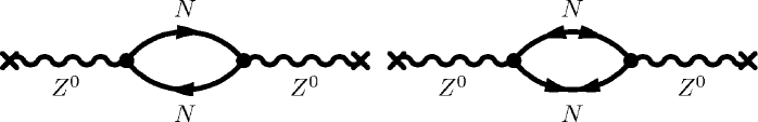
Figure 27: The one-loop contribution to the polarization tensor in the superfluid matter; solid lines refer to the baryon propagators, wavy lines to the (amputated) $Z^{0}$ propagator.

The superfluid in a neutron star can be considered as a two-component system, which, for a fixed density and temperature, consists of paired quasiparticles in the condensate and elementary excitations above the condensate. Their quasi-equilibrium densities are controlled by Cooper pair formation and pair breaking processes. The rate of these reactions are non-exponential in the vicinity of $T_{c}$, however, they are suppressed at asymptotically low temperatures exponentially, because of an exponential decrease of excitations above the condensate. These processes can proceed with the emission of neutrino pairs via the reactions $\{NN\}\rightarrow N+N+\nu+\bar{\nu}$ and $N+N\rightarrow\{NN\}+\nu+\bar{\nu}$, where $\{NN\}$ denotes the Cooper pair, $N$ an excitation. Neutrinos of all three flavors can be emitted in such a process. The corresponding emissivities are  [225]

$$\epsilon_{\nu\bar{\nu}}=\frac{12}{15\pi^{5}}G_{F}^{2}C_{N}p_{FN}m_{N}^{*}T^{7}\left(\frac{\Delta_{N}}{T}\right)^{7}I\left(\frac{\Delta_{N}}{T}\right)\theta(T_{cN}-T),\quad N\in(n,p)$$ (251)

where $C_{n}=\xi_{1}\gamma_{n}^{2}+\xi_{2}g_{A}^{2}\gamma^{2}_{n,\sigma}$ and $C_{p}=\xi_{0}\gamma_{p}^{2}+\xi_{3}$. Here $\xi_{1}=1$, $\xi_{2}=0$ if neutrons are paired in the ${}^{1}S_{0}$ state and $\xi_{1}=2/3$ $\xi_{2}=4/3$ if they are paired in the ${}^{3}P_{2}$ state. Because of their relative low density protons pair in the ${}^{1}S_{0}$ channel and there is only a vector current contribution from protons; the factor $\xi_{3}\sim 1$ takes into account the electromagnetic correlations in the weak vertex. The functions $\gamma_{n/p}$ and $\gamma_{n/p,\sigma}$ take into account the correlations due to the strong force in the vector and axial vector vertices respectively. The temperature dependence of the emissivity $\epsilon_{\nu\bar{\nu}}\propto T^{7}$ is familiar from the analysis of the reaction $n\to n+\nu+\bar{\nu}$ in magnetic fields [Eq. (224)] and is characteristic for the one-body bremsstrahlung process. The remaining parameters in Eq. (251) enter through the density of state of a single fermion. The integral in Eq. (251) is defined as

$$I(x)=\int^{\infty}_{0}\frac{(\mbox{cosh}~{}y)^{5}dy}{[\mbox{exp}(x~{}\mbox{cosh}~{}y)+1]^{2}}\simeq\sqrt{\frac{\pi}{4x}}e^{-2x}.$$ (252)

It can be seen that in the limit $\Delta/T\gg 1$, the rates of the CPBF process are exponentially suppressed, as it is the case for the competing two-nucleon processes. However, because of mild phase space restrictions (phase space volume of a single nucleon) these processes considerably contribute to the total neutrino emissivity at moderate temperatures $T\leq T_{c}$. The magnitude of the CPBF processes is $\epsilon_{\nu\bar{\nu}}\sim 10^{21}\times T_{9}^{7}$.

We now turn to the charged current weak decay Urca process $n\to p+e+\bar{\nu}$ in the superfluid matter and concentrate on the one-loop approximation [200]. This process is described by the first diagram in Fig. (27) with the $Z^{0}$ replaced by $W^{+}$ and $NN=n,p$. The second diagram does not contribute at one-loop.  The vector and axial-vector one-loop polarization tensors have the form

$$i\Pi_{V/A}^{<}(q)=\sum_{\sigma}\int\frac{d^{4}p}{(2\pi)^{4}}G^{<}(p+q)G^{>}(p),$$ (253)

i.e. are identical for the vector and axial vector vertices; explicit evaluation of this expression leads to

$$i\Pi_{V/A}^{<}(q) = \sum_{\sigma}\int\frac{d^{3}p}{(2\pi)^{3}}\Biggl{\{}\left(\frac{u_{p}^{2}u_{k}^{2}}{\omega+\varepsilon_{p}-\varepsilon_{k}+i\delta}-\frac{v_{p}^{2}v_{k}^{2}}{\omega-\varepsilon_{p}+\varepsilon_{k}+i\delta}\right)\left[f(\varepsilon_{p})-f(\varepsilon_{k})\right]$$ (254)

$$+u_{p}^{2}v_{k}^{2}\left(\frac{1}{\omega-\varepsilon_{p}-\varepsilon_{k}+i\delta}-\frac{1}{\omega+\varepsilon_{p}+\varepsilon_{k}+i\delta}\right)\left[f(-\varepsilon_{p})-f(\varepsilon_{k})\right]\Biggr{\}},$$

where $u_{p}^{2}=(1/2)\left(1+\xi_{p}/\varepsilon_{p}\right)$, $u_{p}^{2}+v_{p}^{2}=1$ with $\varepsilon_{p}=\sqrt{\xi_{p}^{2}+\Delta^{2}_{p}}$ and $\xi_{p}$ being the proton single particle spectra in the superfluid and unpaired states; the quantities with the index $k$ refer to the same functions for neutrons. Inspection of the denominators of four terms contributing in Eq. (254) shows that the first two terms correspond to excitations of a particle-hole pair while the last two to excitation of particle-particle and hole-hole pairs. The last term does not contribute to the neutrino radiation rate $(\omega>0)$. We identify the first two terms as scattering ($SC$) terms, while the third term as pair-braking ($PB$) term. For unpaired neutrons and protons $u_{p,k}=1$ and $v_{p,k}=0$, only the first term survives and one recovers the polarization tensor of non-superconducting matter. Upon evaluating the phase space integrals, the neutrino emissivity is written as

$$\epsilon_{\bar{\nu}}=\epsilon_{0}J,\quad J=-\frac{1}{6}\int_{-\infty}^{\infty}\!dy~{}g_{B}(y)\left[I^{SC}+I^{PB}\right]\int_{0}^{\infty}dzz^{3}f_{e}(z-y).,$$

where $\epsilon_{0}$ is defined in Eq. (221). This result differs from its normal state counterpart by the sum of the integrals $I^{SC}+I^{PB}$ which reduces to the logarithm in Eq. (221) for $T\geq T_{c}$.

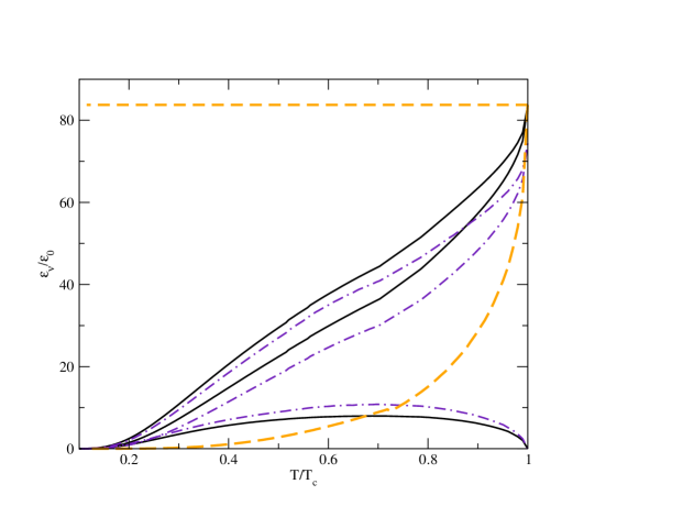
Figure 28: The neutrino emissivity in units of $\epsilon_{0}$ versus temperature (solid lines $\Delta_{n}(0)=\Delta_{p}(0)=0.5$ MeV, dashed-dotted lines $\Delta_{n}(0)=0.5,$ $\Delta_{p}(0)=2$ MeV). The scattering, pair-breaking contributions and their sum are shown by dashed and dashed-dotted and solid lines. The upper short-dashed line is the extrapolation of the rate for unpaired matter to low temperatures, the lower one corresponds to the exponential suppression as discussed in the text.

These integrals are defined as

$$\left(\begin{array}[]{c}I^{SC}\\ I^{PB}\end{array}\right)=\int_{-\infty}^{\infty}dx~{}\left(\begin{array}[]{c}u_{p}^{2}u_{k}^{2}\\ u_{k}^{2}v_{p}^{2}\\ \end{array}\right)\Xi^{SC/PB}\left[f(\pm\sqrt{x^{2}+w_{p}^{2}})-f(\sqrt{x^{2}+w_{p}^{2}}+y)\right]\theta(1-|x_{0}^{\pm}|),$$ (255)

where $x=\beta\xi_{p}$, $w_{i}=\beta\Delta_{i}$ ($i\in n,p$), $y=\beta\omega$ and $\Xi^{SC/PB}=(\omega\pm\varepsilon_{p})/\sqrt{|(\omega\pm\varepsilon_{p})^{2}-\Delta_{n}^{2}|}$; the explicit form of the functions $x^{\pm}_{0}$ is given in ref. [200]. Fig. 28 shows the temperature dependence of the direct Urca neutrino emissivity in the range $0.1\leq T/T_{c}\leq 1$. An important feature seen in this figure is the nearly linear dependence of the emissivity on the temperature in the range $0.1\leq T/T_{c}\leq 1$; the commonly assumed exponential decay - a factor exp($-\Delta/T$) with $\Delta={\rm max}(\Delta_{n},\Delta_{p})$ - underestimates the emissivity. (Similar conclusion concerning the suppression of the direct Urca process by pair correlations were reached in ref. [226] which treated the scattering contribution to the emissivity). The contribution of the pair-breaking processes becomes substantial in the low-temperature range $0.1\leq T/T_{c}\leq 0.4$ where it is about half of the scattering contribution at $T/T_{c}\sim 0.1$. For unequal values of pairing gaps (e.g. $\Delta_{p}=2$, $\Delta_{n}=0.5$ MeV) the emissivity of the scattering process is suppressed, since at a given temperature the phase space accessible to the excited states is reduced. The pair-breaking processes are almost unaffected since they are related to the scattering of particles in and out-of the condensate.

So far our discussion was confined to the case where the nucleons are paired in the ${}^{1}S_{0}$ channel. At high densities, as is well know, neutrons are paired in the ${}^{3}P_{2}$ channel. In this case the gap function is not isotropic in general and may have nodes on the Fermi-surface. The suppression of the phase space of the Urca process was studied in terms of suppression factors ${\cal R}=\epsilon_{\nu}/\epsilon_{0}$. In the case where the gap function has nodes at the Fermi-surface the suppression is a power law [15, 226]. Another possible implication of the $P$-wave superfluidity is the existence of Goldstone modes - collective excitations - which are due to breaking of the rotational invariance by the anisotropic $P$-wave condensate. These Goldstone boson or “angulons”($\alpha$) may couple to the weak neutral current [227]. The process $\alpha+\alpha\to\nu+\bar{\nu}$ leads to an emissivity which scales as $\epsilon_{ang}\propto 10^{17}T_{9}^{9}(0.15/v)^{3}$ erg cm^-3 s^-1 where $v$ is the angulon speed. The high power of temperature in the process is due to the thermal nature of angulons. At moderate temperature $T\leq T_{c}$ the CPBF processes are more efficient than the angulon annihilation; at extreme low temperatures and in the cases where CPBF processes are suppressed exponentially, the angulon annihilation processes may become important.

4 Cooling of neutron stars

The equation of state of dense hadronic matter and the neutrino emissivities discussed in the previous chapters are the key ingredients of cooling simulations of neutron stars. The results of such simulations are combined with the experimental measurements of surface temperatures of neutron stars to gain information on properties of compact stars. In this chapter we review these simulations and their comparison with observational surface temperatures.

Neutrino emissivities control the cooling rate of a neutron star during the first $10^{4}-10^{5}$ yr of their evolution. For later times the photon emission from the surface dominates and the heating in the interior can be a significant factor in maintaining the surface temperature above the observational limit. Depending on the dominant neutrino emission process in the neutrino emission era $t\leq 10^{5}$ yr the cooling proceeds according to the slow (standard) or the fast (nonstandard) scenario [15, 225].

The slow cooling scenario is based on neutrino cooling via the modified Urca and bremsstrahlung processes, modified appropriately to take into account the superfluidity of the star’s interior. The fast cooling scenarios invoke “exotic” cooling mechanism(s), such as the pion/kaon decay processes, the direct Urca process on nucleons or hyperons, as well as their counterparts in deconfined quark phase(s). We have seen that the phase-space arguments are the key to understanding the relative importance of different processes; those leading to fast cooling are characterized by a one body phase space and hence temperature dependences are $\sim T^{6}$ while those responsible for slow cooling originate from two-body processes and their emissivities scale with the temperature as $T^{8}$.

An inspection of the observational data on neutron star surface temperatures, which is commonly presented on a plot of photon-luminosity (or surface temperature) vs age (see Fig. 29 and 30 below) shows that the data cannot be described by a single cooling track; there must be an effective mechanism that regulates the cooling rate in a manner that some of the stars cool faster than others. In particular the Vela pulsar 0833-45 and the radio-silent compact star Geminga have temperatures that are far too low to be accommodated within a model based on slow cooling agents. It is reasonable to assume that the heavier stars cool via some fast mechanism, while the lighter stars cool slowly via the modified processes. The fast cooling agents are effective above a certain density threshold, which could be either the density of phase transitions to a novel state of matter or the density at which kinematical constraints are lifted, as is the case for the Urca process. Such an approach allows one to spread the cooling tracks within a range that can accommodate the currently available data. While such a strategy is a plausible ansatz one should keep in mind that neutron star cooling is a complex, multi-parameter problem and the processes which are actually responsible for fast (and to some extent slow) cooling of neutron stars are not known with certainty.

The thermal evolution is governed by the coupled system of equations for energy balance [228, 229, 230, 231, 232, 233],

$$\frac{\partial(Le^{\nu})}{\partial r} = 4\pi r^{2}e^{\Lambda}\left(-\epsilon_{\nu}e^{\nu}+he^{\nu}-c_{v}\frac{\partial(Te^{\nu}/2)}{\partial t}\right)\,,$$ (256)

and thermal energy transport,

$$\frac{\partial(Te^{\nu/2})}{\partial r} = -\frac{(Le^{\nu})e^{(\lambda-\nu)/2}}{4\pi r^{2}\kappa}\,,$$ (257)

where $L$ is the luminosity, $T$ the temperature. This system requires as a microphysical input the neutrino emissivity $\epsilon_{\nu}(\rho,T)$, the heating rate $h(\rho,T,\Omega,\dot{\Omega})$, with $\Omega$ and $\dot{\Omega}$ being the spin frequency and its derivative, the heat capacity $c_{\mathrm{v}}(\rho,T)$, and the thermal conductivity, $\kappa(\rho,T)$, where $\rho$ is the local density. The boundary conditions for Eqs. (256) and (257) are $L(r=0)=0$ and $T(r=r_{e})=T_{e}$, where $r_{e}$ and $T_{e}$ are radius and temperature of the envelope. The last condition matches the temperature of the star to that of the envelope, since to a good approximation the temperature gradients and heat transport within the envelope are independent of the cooling of the “thermal core” of the star which extends from densities $10^{10}$ g cm^-3 to its center. After the first $10^{2}-10^{3}$ years, the thermal core of the star is isothermal and the cooling of the star is described by Eq. (256) which can be written in terms of quantities which are integrals of the microscopic parameters over the volume of the isothermal core

$$C_{v}\frac{dT}{dt}=-L_{\nu}-L_{\gamma}+H,$$ (258)

where $L_{\nu}$ and $L_{\gamma}$ are the neutrino and photon luminosities, $H$ is the heating rate, and $C_{v}$ is the integrated specific heat of the core. The photon luminosity is given by the black-body radiation formula $L_{\gamma}=4\pi R^{2}\sigma T_{e}^{4}$, where $\sigma$ is the Stephan-Boltzmann constant, $R$ is the radius of the star, $T_{e}$ is the surface temperature. The neutrino cooling era is characterized by the condition $|L_{\nu}|\gg|L_{\gamma}|,|H|$. The specific heat of the star is mainly due to degenerate fermions and scales with the temperature as $C_{v}\sim T$. If there is a single dominant neutrino emission process with known temperature dependence Eq. (258) can be integrated; for typical slow processes (modified Urca, etc) $L_{\nu}\propto T^{8}$ and one obtains $t\propto T^{-6}$; for rapid cooling processes (e.g. direct Urca) $L_{\nu}\propto T^{6}$ and $t\propto T^{-4}$. The photon cooling era is characterized by the condition $|L_{\nu}|\ll|L_{\gamma}|,|H|$. If the heating processes are ignored, the photon luminosity balances the thermal inertia term on the r. h. side of Eq. (258). In more realistic cases the thermal inertia terms can be ignored and the photon luminosity is fully determined by the heating rate, which is a function of time.

4.1 Observational data

Only a small fraction of radio pulsars that are visible through their radio emission have measurable photon fluxes from their surfaces or magnetospheres. A representative sample of 27 pulsars that will be used below to illustrate the constraints on the cooling theories by the observational data is given in Table LABEL:tab:observation. The effective surface temperatures are specified together with their $2\sigma$ error range.

Pulsar	$P$	$\dot{P}$	$\log(\tau)$	$\log(K)$	$\log(T_{\rm eff}^{\infty})$	Category
	[ms]	[$10^{-15}{\rm\,ss}^{-1}$]	[yr]	[s]	[K]
0531+21	33.40	420.96	2.97†	-13.9	$6.18^{+0.19}_{-0.06}$	B
(Crab)
1509-58	150.23	1540.19	3.19	-12.6	$6.11\pm 0.10$	B
0540-69	50.37	479.06	3.22	-13.6	$6.77^{+0.03}_{-0.04}$	B
0002+62	241.81		$\sim 4$†	$\sim-13$	$6.20^{+0.07}_{-0.27}$	A,bb
0833-45	89.29	124.68	$4.3\pm 0.3$†	-14.0	$6.24\pm 0.03$	A,bb
(Vela)					$5.88\pm 0.09$	A,mH
1706-44	102.45	93.04	4.24	-14.0	$6.03^{+0.06}_{-0.08}$	B
1823-13	101.45	74.95	4.33	-14.1	$6.01\pm 0.02$	C
2334+61	495.24	191.91	4.61	-13.0	$5.92^{+0.15}_{-0.09}$	C
1916+14	1181	211.8	4.95	-12.6	$5.93$	D
1951+32	39.53	5.85	5.03	-15.7	$6.14^{+0.03}_{-0.05}$	B
0656+14	384.87	55.03	5.05	-13.7	$5.98\pm 0.05$	A,bb
					$5.72^{+0.06}_{-0.05}$	A,mH
0740-28	167	16.8	5.20	-14.6	$5.93$	D
1822-09	769	52.39	5.37	-13.4	$5.78$	D
0114+58	101	5.84	5.44	-15.2	$5.98\pm 0.03$	C
1259-63	47.76	2.27	5.52	-16.0	$5.88$	C
0630+18	237.09	10.97	5.53	-14.6	$5.76^{+0.04}_{-0.08}$	A,bb
(Geminga)					$5.42^{+0.12}_{-0.04}$	A,mH
1055-52	197.10	5.83	5.73	-14.9	$5.90^{+0.06}_{-0.12}$	A,bb
0355+54	156.38	4.39	5.75	-15.2	$5.98\pm 0.04$	C
0538+28	143.15	3.66	5.79	-15.3	$5.83$	C
1929+10	226.51	1.16	6.49	-15.6	$5.52$	B
1642-03	388	1.77	6.54	-15.2	$6.01\pm 0.03$	C
0950+08	253.06	0.23	7.24	-16.3	$4.93^{+0.07}_{-0.05}$	B
0031-07	943	0.40	7.56	-15.4	$5.57$	D
0751+18	3.47	$7.9\times 10^{-4}$	7.83	-20.6	$5.66$	C
0218+42	2.32	$8.0\times 10^{-5}$	8.66	-21.7	$5.78$	C
1957+20	1.60	$1.7\times 10^{-5}$	9.18	-22.6	$5.53$	C
0437-47	5.75	$3.8\times 10^{-5}$	9.20	-21.7	$5.94\pm 0.03$	B

Table 5: Sample of observed data. The entries are: rotation period $P$ and period derivative $\dot{P}$, spin-down age $\tau=P/2\dot{P}$, $K=P\dot{P}$ and effective (redshifted) surface temperature $T_{\rm eff}^{\infty}$; bb and mH refer to blackbody and magnetized hydrogen atmosphere fits; $\dagger$ refers to known true age rather than the spin-down age.

The ages of the pulsars listed in Table LABEL:tab:observation are their spin-down ages, $\tau=P/2\dot{P}$, except the PSRs 0531+21 (Crab), 0833-45 (Vela) and 0002+62, for which the age is know either through historical records (Crab pulsar) or the age of the supernova remnant they are embedded in. The spin-down age assumes that the star decelerates under the action of magnetic dipole radiation with a constant, time independent rate. If we write the star’s spin-down rate as

$$\dot{\Omega}(t)=K(t)\Omega^{n}(t),$$ (259)

where $\Omega$ is the spin frequency and $n$ is the breaking index, the assumption above translates to $K=$ const and $n=3$. The spin-down age approximates the true age of a pulsar within an accuracy of a factor of 3 or so. The sample of pulsars in Table LABEL:tab:observation is divided in four categories depending on a number of observational and fitting features. Four pulsars that belong to category D have not been detected in the soft $X$-ray range. The sensitivity of instruments sets an upper limit for the surface temperature. The data from ten pulsars of category C contain too few photons for spectral fits. The surface temperatures for these objects were obtained by using the totally detected photon flux. The spectra of eight pulsars of category B, which include the Crab pulsar 0531+21, can be fitted either (i) by a power-law spectrum or (ii) by a blackbody spectrum with high temperature and small effective area, much smaller than a neutron star surface. Presumably, their $X$-ray emission is dominated by magnetospheric emission. Therefore, the temperatures, determined from the spectral fits, are probably higher than the actual surface temperatures. Finally, there are five pulsars of category A, 0833-45 (Vela), 0656+14, 0002+62, 0630+18 (Geminga), and 1055-52, whose spectrum can be fitted by a two-component fit. The soft blackbody component is attributed to the surface emission, while the hard blackbody (or power-law) component is attributed to the magnetospheric emission. These pulsars are marked with error bars in Figs. 29 and 30.

4.2 Cooling simulations

Figure 29 shows the cooling of a family of neutron stars with masses in the range 1.0 to 1.9 $M_{\odot}$ featuring the same microphysical ingredients [230]. Baryonic matter is paired below the critical temperatures of the superfluid phase transition which are of the order of $10^{9}$ K; a phase transition to the pion condensed phase at the density $n_{c}=3n_{0}$ is assumed. The Cooper pair-breaking/formation processes (CPBF) are not included in the simulation. The initial phase of the cooling for $0\leq t\leq 10^{2}$ yr is independent of the assumed value of the temperature at $t=0$. At this stage, the star supports temperature gradients throughout the thermal core. The first kink in the cooling curves at $t\sim 10^{2}$ marks the point where the cooling wave, which propagates outwards from the center of the star, reaches the surface. During the entire subsequent evolution the thermal core is isothermal and the slope of the cooling curves within the era $10^{2}\leq t\leq 10^{5}$ yr is determined by the dominant neutrino emission mechanism(s).

Figure 29: Dependence of surface photon luminosity on the age [230]. The model includes pion condensation at high densities; the CPBF processes are switched off. The right panel includes pion mode softening effects in the modified Urca process [201] while the left panel is based on OPE result of ref. [207].

The second kink at $t\simeq 10^{5}$ yr marks the point where the transition from the neutrino dominated cooling to photon dominated cooling occurs. The change in the slope is due to the difference in the temperature dependence of the photon and neutrino cooling rates. The neutrino dominated cooling era is independent of the initial temperature assumed at the instance when the star become isothermal (unless this temperature is unrealistically low); in contrast, the initial conditions for the photon cooling dominated era strongly depends on the cooling pre-history of the star.

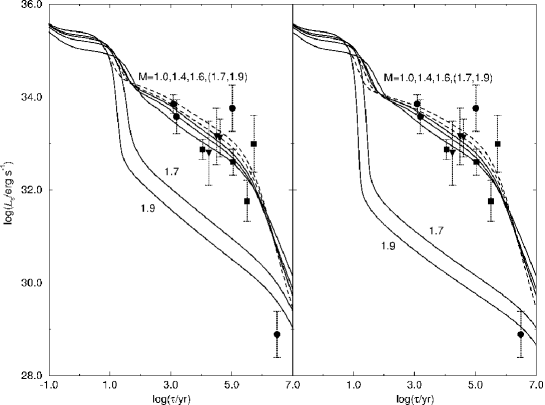
Figure 30: Dependence of surface photon luminosity on the age. The CPBF processes are included in all graphs. From left to right: the model includes pion condensation, the model includes in addition the Urca process; the model features neutron gap reduced by factor 6. [230, 231].

The late time asymptotics of cooling in the photon dominated era is mainly determined by the models of the non-isothermal envelope which relate the temperature of the isothermal core to the surface temperature; the core temperature drops across the envelope by roughly two orders of magnitude. The late time asymptotics of cooling is likely to be dominated by the heating in the interior of the star.

Let us now concentrate on the neutrino dominated cooling era. The qualitatively different behavior of stars with masses $M>1.6M_{\odot}$ and $M<1.6M_{\odot}$ arises from the fact that the former feature a pion condensate, since their central densities are larger than the threshold density for pion condensation. This segregation of the cooling tracks into high-temperature and low-temperature ones is common to the cooling theories with slow and fast cooling agents. An inspection of the observational data, shows that the neutrino dominated era cannot be fitted by a single track and a mechanism is needed to provide a smooth crossover from slow to rapid cooling. One possibility is the “threshold mechanism” in which some of the (low mass) stars have central densities below a threshold for a fast processes, and thus cool slow, while others, more massive, above this threshold and thus cool fast. Such mechanism is unsatisfactory, since one will need an extreme fine tuning of masses of neutron stars to accommodate the data (see e. g. Fig. 29). It should be noted that any phase transition (as, e.g., pion or kaon condensation) or kinematically constrained process (such as the direct Urca process) will have precursors, where the fluctuations below the transition density will transform the sharp transition into a smooth crossover. The effects of such a precursor for the case of pion condensation, the so called pion mode softening, and its effect on cooling is studied in refs. [230, 233].

A more interesting (and realistic) mechanism of the crossover from slow to fast cooling is offered by the CPBF processes. The variations in the cooling rates introduced by these processes arise due to the fact that the density profiles of pairing gaps for baryons map differently on the density profiles of light and massive stars. This effect is demonstrated in Fig. 30 where the models presented in Fig. 29 are supplemented by the CPBF processes. The leftmost panel shows the effect of including the CPBF process in the presence of pion condensate, while the next plot to the right shows the effect of adding the direct Urca process. While the segregation between the high and low mass objects remain, the cooling tracks of low mass objects are now spread in a certain range.

A wider range of surface temperatures can be covered upon suppressing (artificially) the neutron ${}^{3}P_{2}$ gaps by a factor of a few. In this case, the matter is unpaired at high-densities and the star cools as partially superfluid object. One may conclude that not only the magnitudes of the gaps are important, but also the density profiles over which they are spread [15, 16, 232, 233].

Cooling simulations that do not include the heating processes in the interiors of compact stars fail to account for the highest temperatures in the sample of $X$-ray emitting pulsars. It is very likely that the late time evolution of compact stars including the entire photon cooling era and partially the neutrino cooling era are significantly affected by the heating processes in the star’s interior. The heating processes can be roughly divided into three categories: (i) the heating due to the frictional motion of neutron and proton vortices in the superfluids; (ii) the heating that arises due to the local deviations of matter composition from $\beta$-equilibrium; (iii) the heating due to mechanical processes in the solid regions of the star (crust cracking, etc.). Describing these processes will require a detailed account of the physics of neutron star interiors on the mesoscopic scales and is beyond the scope of this article (see ref. [231] for details).

5 Concluding remarks

This review covered a number of topics that are relevant to the theory of compact stars, in particular the physics of hadronic matter with baryonic degrees of freedom and weak interaction processes involving hadrons. It should be clear from the presentation that despite the enormous progress achieved during the past decade, the theory is far from being completed and a large number of exciting topics remain to be studied in the future.

Compact stars continue to pose an enormous intellectual challenge to the physics and astrophysics communities. Rapid progress during the last four decades since the discovery of the first pulsar is an evidence of the vitality of this field. Current and planned observational programs continue the exploration of compact objects in the electromagnetic spectrum; studies of compact stars through gravity waves may become possible in the near future. All this provides an excellent basis for future theoretical studies of compact stars.

References

- [1] S. Chandrasekar, An Introduction to the Study of Stellar Structure, (University of Chicago Press, Chicago, 1939).
- [2] A. Hewish, J. S. Bell, J. D. H. Pilkington, P. F. Scott, and R. A. Collins, Nature 217 (1968) 709.
- [3] R. A. Hulse and J. H. Taylor, Astrophys. J. Lett. 195 (1975) L51.
- [4] J. Schwinger, J. Math. Phys. 2 (1961) 407.
- [5] L. Kadanoff and G. Baym, Quantum Statistical Mechanics, (Benjamin, New York, 1962).
- [6] L. V. Keldysh, Sov. Phys. JETP 20 (1965) 1018 [Zh. Eksp. Theor. Phys. 47 (1964) 1515].
- [7] A. A. Abrikosov, L. P. Gorkov, and I. E. Dzyaloshinski, Methods of Quantum Field Theory in Statistical Physics (Prienice-Hall, Englewood Cliffs, NJ, 1963) (Dover, New York, 1975).
- [8] S. L. Shapiro and S. A. Tuekolsky, Black Holes, White Dwarfs and Neutron Stars: The Physics of Compact Objects (John Willey & Sons, New York, 1983).
- [9] Ia. B. Zeldovich and I. D. Novikov, Stars and Relativity (Dover, New York, 1997).
- [10] G. S. Saakyan, Equilibrium Configurations of Degenerate Gaseous Masses (John Willey & Sons, New York, 1973).
- [11] N. K. Glendenning, Compact Stars: Nuclear Physics, Particle Physics, and General Relativity, 2nd ed. (Springer-Verlag, New York, 2000).
- [12] F. Weber, Pulsars as Astrophysical Laboratories for Nuclear and Particle Physics, (IOP Publishing, Bristol, 1999).
- [13] D. Blaschke, N. K. Glendenning, and A. Sedrakian, Physics of Neutron Star Interiors, Lecture Notes in Physics, vol. 578 (Springer-Verlag, New York, 2001).
- [14] F. Weber, Prog. Part. Nucl. Phys. 54 (2005) 193.
- [15] D. Page, U. Geppert, and F. Weber, Nucl. Phys. A., in press.
- [16] D. G. Yakovlev and C. J. Pethick, Ann. Rev. Astron. Astrophys. 42 (2004) 169.
- [17] M. Prakash, J. M. Lattimer, R. F. Sawyer, and R. R. Volkas, Ann. Rev. Nucl. Part. Sci. 51 (2001) 295.
- [18] D. Rischke, Prog. Part. Nucl. Phys. 52 (2004) 197.
- [19] M. Alford, Prog. Theor. Phys. Suppl. 153 (2004) 1.
- [20] K. Rajagopal and F. Wilczek, At the Frontier of Particle Physics, 3 (2001) 2061; hep-ph/0011333.
- [21] M. Baldo, Nuclear methods and the nuclear equation of state, Int. Rev. of Nucl. Phys. Vol. 8 (World Scintific, Singapore, 1999).
- [22] J. M. Lattimer and M. Prakash, Phys. Rept. 333 (2000) 121.
- [23] H. Heiselberg and M. Hjorth-Jensen, Phys. Rept. 328 (2000) 237.
- [24] P. C. Martin and J. Schwinger, Phys. Rev. 115 (1959) 1342.
- [25] D. C. Langreth and J. W. Wilkins, Phys. Rev. B 6 (1972) 3189.
- [26] W. Botermans and R. Malfliet, Phys. Rep. 198 (1990) 115.
- [27] R. Zimmermann and H. Stolz, Phys. Stat. Sol. (b) 131 (1985) 151.
- [28] M. Schmidt, G. Röpke and H. Schulz, Ann. Phys. (NY) 202 (1990) 57.
- [29] A. Sedrakian and G. Röpke, Ann. Phys. (NY) 266 (1998) 524.
- [30] V. Špička, P. Lipavský, and K. Morawetz, Phys. Rev. B 55 (1997) 5095.
- [31] V. Špička and P. Lipavský, Phys. Rev. B 52 (1995) 14615.
- [32] A. Ramos, A. Polls, and W. H. Dickhoff, Nucl. Phys. A 503 (1989) 1.
- [33] A. Ramos, W. H. Dickhoff, and A. Polls, Nucl. Phys. A 43 (1991) 2239.
- [34] M. Baldo, I. Bombaci, G. Giansiracusa, U. Lombardo C. Mahaux, and R. Sartor, Nucl. Phys. A 545 (1992) 741.
- [35] W. H. Dickhoff and H. Müther, Rep. Prog. Phys. 55 (1992) 1947.
- [36] A. Polls, A. Ramos, J Ventura, S. Amari, and W. H. Dickhoff, Phys. Rev. C 49 (1994) 3050.
- [37] H. Müther, A. Polls, A., and W. H. Dickhoff, Phys. Rev. C 51 (1995) 3040.
- [38] H. Müther, G. Knehr, and A. Polls, Phys. Rev. C 52 (1995) 2955.
- [39] A. Schnell, T. Alm, and G. Röpke, Phys. Lett. B 387 (1996) 443.
- [40] T. Alm, G. Röpke, A. Schnell, N. H. Kwong, and H. S. Köhler, Phys. Rev. C 53 (1996) 2181.
- [41] P. Bozek, Phys. Rev. C 59 (1999) 2619; ibid 65 (2002) 054306.
- [42] P. Bozek and P. Czerski, Phys. Rev. C 66 (2002) 027301.
- [43] Y. Dewulf, D. van Neck, and M. Waroquier, Phys. Lett. B 510 (2001) 89.
- [44] Y. Dewulf, W. H. Dickhoff, D. van Neck, E. R. Stoddard, and M. Waroquier, Phys. Rev. Lett. 90 (2004) 152501.
- [45] Kh. S. Hassaneen and H. Müther, Phys. Rev. C 70 (2004) 054308.
- [46] A. Rios, A. Polls, H. Muther, Phys. Rev. C 73 (2006) 024305.
- [47] N. M. Hugenholtz and L. Van Hove, Physica 23 (1958) 525.
- [48] T. Alm, B. L. Friman, G. Röpke, and H. Schulz, Nucl. Phys. A 551 (1993) 45.
- [49] A. Sedrakian, G. Röpke, and Th. Alm, Nucl. Phys. A 594 (1995) 355.
- [50] T. Alm, G. Röpke, A. Sedrakian and F. Weber, Nucl. Phys. A 604 (1996) 491.
- [51] A. Sedrakian, T. Alm, and U. Lombardo, Phys. Rev. C 55 (1997) R582.
- [52] A. Sedrakian and U. Lombardo, Phys. Rev. Lett. 84 (2000) 602.
- [53] A. Sedrakian, Phys. Rev. C 63 (2001) 025801.
- [54] U. Lombardo, P Nozières, P. Schuck, H.-J. Schulze, and A. Sedrakian, Phys. Rev. C 64 (2001) 064314.
- [55] A. I. Akhiezer, A. A. Isayev, S. V Peletminsky, and A. A. Yatsenko, Phys. Rev. C 63 (2001) 021304.
- [56] H. Müther and A. Sedrakian, Phys. Rev. Lett. 88 (2002) 252503.
- [57] A. A. Isayev, Phys. Rev. C 65 (2002) 031302.
- [58] H. Müther, and A. Sedrakian, Phys. Rev. C 67 (2003) 015802.
- [59] M. Alford, G. Good, S. Reddy, Phys. Rev. C 72 (2005) 055801.
- [60] U. Lombardo and H.-J. Schulze, Lecture Notes in Physics, vol. 578 pg. 30 (Springer, Berlin, 2001).
- [61] D. J. Dean and M. Hjorth-Jensen, Rev. Mod. Phys. 75 (2003) 607.
- [62] A. Sedrakian, D. Blaschke, G Röpke, and H. Schulz, Phys. Lett. B 338 (1994) 111.
- [63] H.-J. Schulze, A. Schnell, G. Röpke, and U. Lombardo, Phys. Rev. C 55 (1997) 0306.
- [64] A. Schnell, G. Röpke, U. Lombardo, and H.-J. Schulze, Phys. Rev. C 57 (1998) 806.
- [65] W. H. Dickhoff, C. C. Gearhart, E. P. Roth, A. Polls, and A. Ramos, Phys. Rev. C 60 (1999) 064319.
- [66] Bao-An Li, P. Danielewicz, and W. G. Lynch, Phys. Rev. C 71 (2005) 054603.
- [67] A. Sedrakian et al (2006) in preparation.
- [68] G. V. Skorniakov and K. A. Ter-Martirosian, Sov. Phys. JETP 4 (1957) 648.
- [69] L. D. Faddeev, Sov. Phys. JETP 12 (1961) 1014.
- [70] H. A. Bethe, Phys. Rev. 138 (1965) B804; ibid 158 (1967) 941.
- [71] P. Schuck, F. Villars, and P. Ring, Nucl. Phys. A 208 (1973) 302.
- [72] J. Dukelsky and P. Schuck, Nucl. Phys. A 512 (1990) 466 .
- [73] A. N. Kvinikhidze and B. Blankleider, Phys. Rev. C 72 (2005) 054001.
- [74] O. Alt, P. Grassberger and W. Sandhas, Nucl. Phys. B 2 (1967) 167.
- [75] M. Beyer, G. Röpke and A. Sedrakian, Phys. Lett. B 376 (1996) 7.
- [76] M. Beyer, W. Schadow, C. Kuhrts, and G. Röpke, Phys. Rev. C 60 (1999) 034004.
- [77] A. Sedrakian and J. W. Clark, Phys. Rev. C, in press, nucl-th/0511076.
- [78] G. E. Beth and E. Uhlenbeck, Physcia 3 (1936) 729; ibid. 4 (1937) 915.
- [79] K. A. Brueckner, Phys. Rev. 96 (1954) 588.
- [80] K. A. Brueckner and C. A. Levinson, Phys. Rev. 97 (1954) 1344.
- [81] K. A. Brueckner and J. L. Gammel, Phys. Rev. 109 (1954) 1023.
- [82] H. A. Bethe and J. Goldstone, Proc. R. Soc. London A 238 (1956) 551.
- [83] H. A. Bethe, B. H. Brandow and A. G. Petschek, Phys. Rev. 129 (1963) 225.
- [84] H. A. Bethe, Ann. Rev. Nucl. Part. Sci. 21 (1971) 93.
- [85] G. Brown, Rev. Mod. Phys. 43 (1971) 1.
- [86] B. D. Day, Rev. Mod. Phys. 39 (1967) 719.
- [87] B. D. Day, Phys. Rev. C 24 (1981) 1203.
- [88] H. Q. Song, M. Baldo, G. Giansiracusa, and U. Lombardo, Phys. Rev. Lett. 81 (1998) 1584.
- [89] M. Baldo, A. Fiasconaro, H. Q. Song, G. Giansiracusa, and U. Lombardo, Phys. Rev. C 65 (2001) 017303.
- [90] R. Sartor, Phys. Rev. C 68 (2003) 057301.
- [91] D. Kaplan and A. Nelson, Phys. Lett. B 175 (1986) 57.
- [92] J. D. Walecka, Theoretical Nuclear and Subnuclear Physics (Oxford University Press, Oxford, 1995).
- [93] B. D. Serot and J. D. Walecka, Adv. Nucl. Phys. 16 (1986) 1.
- [94] F. Gross, Phys. Rev. 186 (1969) 1448.
- [95] A. A. Logunov and A. N. Tavkhelidze, Nuovo Cim. 29 (1963) 380.
- [96] R. Blankenbecler and R. Sugar, Phys. Rev. 142 (1966) 1051.
- [97] R. H. Thompson, Phys. Rev. D 1 (1970) 110.
- [98] A. Amorim and J. A, Tjon, Phys. Rev. Lett. 68 (1992) 772.
- [99] M. R. Anastasio, L. S. Celenza, W. S. Pong, and C. M. Shakin, Phys. Rep. 100 (1983) 327.
- [100] C. J. Horowitz and D. B. Serot, Nucl. Phys. A 464 (1987) 613.
- [101] R. Machleidt, K. Holinde, and Ch. Elster, Phys. Rep. 149 (1987) 1.
- [102] F. de Jong and R. Malfliet, Phys. Rev. C 44 (1991) 998.
- [103] L. Engvik, M. Horth-Jensen, E. Osnes, G. Bao, and E. Ostgaard, Phys. Rev. Lett. 73 (1994) 2650.
- [104] H. Huber, F. Weber, and M. K. Weigel, Phys. Rev. C 50 (1994) 1287.
- [105] H. Huber, F. Weber, and M. K. Weigel, Phys. Rev. C 51 (1995) 1790.
- [106] F. de Jong and H. Lenske, Phys. Rev. C 58 (1998) 890.
- [107] T. Gross-Boelting, C. Fuchs, and Amand Faessler, Nucl. Phys. A 648 (1998) 105.
- [108] E. Schiller and H. Müther, Eur. Phys. J. A 11 (2001) 15.
- [109] D. Alonso and F. Sammarruca, Phys. Rev. C 67 (2003) 054301.
- [110] E. N. E. van Dalen, C. Fuchs, and Amand Faessler, Nucl. Phys. A 744 (2004) 227.
- [111] A. E. L. Dieperink, Y. Dewulf, D. van Neck, M. Waroquier, and V. Rodin, Phys. Rev. C 68 (2003) 064307.
- [112] H. Müther, M. Prakash, and T. L. Ainsworth, Phys. Lett. B 199 (1987) 469.
- [113] C.-H. Lee, T. T. S. Kuo, G. Q. Li, and G. E. Brown, Phys. Rev. C 57 (1998) 3488.
- [114] A. Akmal, V. R. Pandharipande, and D. G. Ravenhall, Phys. Rev. C 58 1804 (1998).
- [115] X. R. Zhou, G. F. Burgio, U. Lombardo, H.-J. Schulze, and W. Zuo, Phys. Rev. C 69 (2004) 018801.
- [116] S. A. Coon et al., Nucl. Phys. A 317 (1979) 242.
- [117] P. Grangé, A. Lejeune, M. Martzolff, and J.-F. Mathiot, Phys. Rev. C 40 (1989) 1040.
- [118] W. Zuo, A. Lejeune, U. Lombardo, and J.-F. Mathiot, Eur. Phys. J. A 14 (2002) 469; Nucl. Phys. A 706 (2002) 418.
- [119] B. S. Pudliner, V. R. Pandharipande, J. Carlson, and R. B. Wiringa, Phys. Rev. Lett. 74 (1995) 4396.
- [120] B. S. Pudliner, V. R. Pandharipande, J. Carlson, S. C. Pieper, and R. B. Wiringa, Phys. Rev. Lett. 62 (1997) 014001.
- [121] V. A. Ambartsumyan and G. S. Saakyan, Sov. Astron-AJ 4 (1960) 187 [Astron. Zhur. 37 (1960) 193.]
- [122] A. Reuber, K. Holinde, and J. Speth, Nucl. Phys. A 500 (1989) 485.
- [123] P. M. M. Maessen, Th. A. Rijken, and J. J. de Swart, Phys. Rev. C 40 (1989) 2226.
- [124] Th. A. Rijken, V. G. J. Stoks, and Y. Yamamoto, Phys. Rev. C 59 (1999) 21.
- [125] V. G. J. Stoks and Th. A. Rijken, Phys. Rev. C 59 (1999) 3009.
- [126] B. F. Gibson, I. R. Afnan, J. A. Carlson, and D. R. Lehman, Prog. Theor. Phys. Suppl. 117 (1994) 339.
- [127] A. R. Bodmer, D. M. Rote, and A. L. Mazza, Phys. Rev. C 2 (1972) 1623.
- [128] S. Nagata and H. Bando, Prog. Theor. Phys. 72 (1984) 113.
- [129] Y. Yamamoto, H. Bando, and J. Zofka, Prog. Theor. Phys. 80 (1988) 757.
- [130] Y. Yamamoto and H. Bando, Prog. Theor. Phys. 83 (1990) 254.
- [131] V. R. Pandharipande, Nucl. Phys. A 178 (1971) 123.
- [132] H. A. Bethe and M. B. Johnson, Nucl. Phys. 230 (1974) 1.
- [133] N. K. Glendenning, Astrophys. J. 293 (1985) 470.
- [134] F. Weber and M. Weigel, Nucl. Phys. A 493 549 (1989); ibid 495 (1989) 363c.
- [135] N. K. Glendenning, F. Weber, and S. A. Moszkowski, Phys. Rev. C 45 (1992) 844.
- [136] N. K. Glendenning and S. A. Moszkowski, Phys. Rev. Lett. 67 (1991) 2414.
- [137] M. Baldo, G. F. Burgio, and H.-J. Schulze, Phys. Rev. C 61 (2000) 055801l; ibid 58 (1998) 3688.
- [138] I. Vidana, A. Polls, A. Ramos, L. Engvik, and M. Hjorth-Jensen, Phys. Rev. C 62 (2000) 035801.
- [139] A. Rios, A. Polls, A. Ramos, and I. Vidana, Phys. Rev. C 72 (2005) 024316.
- [140] O. E. Nicotra, M. Baldo, G. F. Burgio, and H.-J. Schulze, nucl-th/0506066.
- [141] A. B. Migdal, E. E. Saperstein, M. A. Troitsky, and D. N. Voskresensky, Phys. Rep. 192 (1990) 179.
- [142] W. Dickhoff, J. Meyer-ter-Vehn, H. Müther, and A. Faessler, Nucl. Phys. A 368 (1981) 445.
- [143] W. Dickhoff, J. Meyer-ter-Vehn, H. Müther, and A. Faessler, Phys. Rev. C 23 (1981) 1154.
- [144] V. F. Dmitriev and T. Suzuki, Nucl. Phys. A 438 (1985) 697.
- [145] T. Wakasa et al, Phys. Rev. C 55 (1997) 2909.
- [146] T. Suzuki and H. Sakai, Phys. Lett. B 455 (1999) 25.
- [147] G. E. Brown and H. A. Bethe, Astrophys. J. 432 (1994) 659.
- [148] J. R. Oppenheimer and G. M. Volkoff, Phys. Rev. 55 (1939) 374.
- [149] R. B. Wiringa, V. Fiks, and A. Fabrocini, Phys. Rev. C 38 (1988) 1010.
- [150] J. Negele and D. Vautherin, Nucl. Phys. A 207 298 (1973).
- [151] G. Baym, C. Pethick, and P. Sutherland, Astrophys. J 170 (1971) 299.
- [152] N. Stergioulas and J. L. Friedman Astrophys. J 492 (1998) 301.
- [153] D. J. Nice, E. M. Splaver, I. H. Stairs, O. Löhmer, A. Jessiner, M. Kramer, and J. M. Cordes, Astrophys. J. 634 (2005) 1242.
- [154] J. B. Hartle and D. Sharp, Astrophys. J. 150 (1967) 1005.
- [155] J. B. Hartle, Astrophys. J. 150 (1967) 1005.
- [156] J. B. Hartle and K. S. Thorn, Astrophys. J. 153 (1968) 807.
- [157] D. M. Sedrakian and E. V. Chubarian, Astrofizika, 4 (1968) 239; ibid. 551.
- [158] D. M. Sedrakian, V. V. Papoian, and E. V. Chubarian, Mon. Not. RAS 149 (1970) 25.
- [159] F. Weber, N. K. Glendenning, and M. K. Weigel, Astrophys. J, 373 (1991) 579.
- [160] R. B. Wiringa, Rev. Mod. Phys. 65 (1993) 231.
- [161] R. B. Wiringa and S. C. Pieper, Phys. Rev. Lett. 89 (2002) 182501.
- [162] J. Carlson, J. Morales, Jr., V. R. Pandharipande, and D. G. Ravenhall, Phys. Rev. C 68 (2003) 025802.
- [163] F. Pederiva, A. Sarsa, K.E. Schmidt, and S. Fantoni, Nucl. Phys. A 742 (2004) 255.
- [164] A. Sarsa, S. Fantoni, K. E. Schmidt, and F. Pederiva, Phys. Rev. C 68 (2003) 024308.
- [165] M. Lutz, B. Friman, and Ch. Appel, Phys. Lett. B 474 (2000) 7.
- [166] N. Kaiser, S. Fritsch, and W. Weise, Nucl. Phys. A 697 (2002) 255.
- [167] S. Fritsch, N. Kaiser, and W. Weise, Phys. Lett. B 545 (2002) 73.
- [168] P. Finelli, N. Kaiser, D. Vretenar, and W. Weise nucl-th/0509040.
- [169] E. Epelbaum, nucl-th/0509032.
- [170] P. Ring, Lecture Notes in Physics, vol. 641 pg. 175, (Springer, Berlin, 2004).
- [171] R. J. Furnstahl, H.-B. Tang, and B. D. Serot, Phys. Rev. C 52 (1995) 1368.
- [172] R. J. Furnstahl, Lecture Notes in Physics, vol. 641 pg. 1, (Springer, Berlin, 2004).
- [173] B. Serot, ibid pg. 31.
- [174] H.-M. Müller, S. E. Koonin, R. Seki, and U. van Kolck, Phys. Rev. C 61 (2000) 044320.
- [175] D. Lee and T. Schaefer, Phys. Rev. C 72 (2005) 024006
- [176] D. Lee and T. Schaefer, nucl-th/0509017; nucl-th/0509018.
- [177] J.-W. Chen and D. B. Kaplan, Phys. Rev. Lett. 92 (2004) 257002.
- [178] A. Sedrakian, H. Müther, and P. Schuck, Nucl. Phys. A, in press.
- [179] H. Müther and A. Polls, Prog. Part. Nucl. Phys. 45 (2000) 243.
- [180] K. Kowalski, D. J. Dean, M. Hjorth-Jensen, T. Papenbrock, and P. Piecuch, Phys. Rev. Lett. 92 (2004) 132501.
- [181] D. J. Dean, et al, Nucl.Phys. A 752 (2005) 299.
- [182] S. R. Beane, P. F. Bedaque, W. C. Haxton, D. R. Phillips, M. J. Savage, nucl-th/0008064.
- [183] P. F. Bedaque and U. van Kolck, Ann. Rev. Nucl. Part. Sci. 52 (2002) 339.
- [184] D. B. Kaplan, nucl-th/0510023.
- [185] R. J. Furnstahl and H.-W. Hammer, Ann. Phys. 302 (2002) 206.
- [186] T. Schaefer, C.-W. Kao, and S. R. Cotanch, Nucl. Phys. A 762 (2005) 82.
- [187] G. Gamow and M. Schoenberg, Phys. Rev. 59 (1941) 539.
- [188] J. Boguta, Phys. Lett. B 106 (1981) 255.
- [189] J. M. Lattimer, C. J. Pethick, M. Prakash, and P. Haensel, Phys. Rev. Lett. 66 (1991) 2701.
- [190] C. J. Pethick, Rev. Mod. Phys. 64 (1992) 1133.
- [191] A. Sedrakian and A. Dieperink, Phys. Lett. B 463 (1999) 145.
- [192] H. Y. Chiu and E. E. Salpeter, Phys. Rev. Lett. 12 (1964) 413.
- [193] J. N. Bahcall and R. A. Wolf, Phys. Rev. Lett. 14 (1965) 343; Phys. Rev. 140 (1965) B1452.
- [194] M. Prakash, M. Prakash, J. M. Lattimer, and C. J. Pethick, Astrophys. J. 390 (1992) L77.
- [195] O. V. Maxwell, Astrophys. J. 316 (1987) 691.
- [196] T. Tatsumi, T. Takatsuka, and R. Tamagaki, Prog. Theor. Phys. 110 (2003) 179.
- [197] E. G. Flowers, M. Ruderman, and P. G. Sutherland, Astrophys. J. 205 (1976) 541.
- [198] D. N. Voskresensky and A. V. Senatorov, Sov. J. Nucl. Phys. 45 (1987) 411 [ Yad. Fiz. 45 (1987) 657].
- [199] D. G. Yakovlev, A. D. Kaminker, and K. P. Levenfish, Astron. Astrophys. 343 (1999) 650.
- [200] A. Sedrakian, Phys. Lett. B 607 (2005) 27.
- [201] D. N. Voskresensky and A. V. Senatorov, Sov. Phys. JETP 63 (1986) 885.
- [202] A. Sedrakian and A. E. L. Dieperink, Phys. Rev. D 62 (2000) 083002.
- [203] D. Lai, Rev. Mod. Phys. 73 (2001) 629.
- [204] E. N. E. van Dalen, A. E. L. Dieperink, A. Sedrakian, and R. G. E. Timmermans, Astron. Astrophys. 360 (2000) 549.
- [205] L. B. Leinson and A. Perez, JHEP 9 (1998) 20.
- [206] D. A. Baiko and D. G. Yakovlev, Astron. Atrophys. 342 (1999) 192.
- [207] B. L. Friman and O. V. Maxwell, Astrophys. J. 232 (1979) 541.
- [208] T. Ericson and J.-F. Mathiot, Phys. Lett. B 219 (1989) 507.
- [209] E. N. E. van Dalen, A. E. L. Dieperink, and J. A. Tjon, Phys. Rev. C 67 (2003) 065807.
- [210] A. Schwenk, P. Jaikumar, and C. Gale, Phys. Lett. B 584 (2004) 241.
- [211] M. L. Ter-Mikaelian, Zh. Exp. Teor. Fiz. 25 (1953) 289; ibid. 296.
- [212] S. Klein, Rev. Mod. Phys. 71 (1999) 1501.
- [213] L. D. Landau and I. Ya. Pomeranchuk, Dokl. Akad. Nauk SSSR 92 (1953) 535; ibid. 92 (1953) 375.
- [214] A. B. Migdal, Phys. Rev. 103 (1956) 1811.
- [215] J. Knoll and D. N. Voskresensky, Ann. Phys. 249 (1996) 532.
- [216] P. Bozek, J. Margueron, and H. Müther, Ann. Phys. 318 (2005) 245.
- [217] E. Olsson and C. J. Pethick, Phys. Rev. C 66 (2002) 065803.
- [218] G. I. Lykasov, E. Olsson, and C. J. Pethick, Phys. Rev. C 72 (2005) 025805.
- [219] R. G. E. Timmermans, A. Yu. Korchin, E. N. E. van Dalen, and A. E. L. Dieperink Phys. Rev. C 65 (2002) 064007.
- [220] C. Hanhart, D. R. Phillips, and S. Reddy, Phys.Lett. B 499 (2001) 9.
- [221] C. Hanhart, D. R. Phillips, S. Reddy, and M. J. Savage, Nucl. Phys. B 595 (2001) 335.
- [222] S. Cullen and M. Perelstein Phys. Rev. Lett. 83 (1999) 268.
- [223] N. Arkani-Hamed, S. Dimopoulos, and G. Dvali, Phys. Lett. B 429 (1998) 263; Phys. Rev. D 59 (1999) 086004.
- [224] T. Han, J. D. Lykken, and R.-J. Zhang, Phys. Rev. D 59 (1999) 105006.
- [225] D. N. Voskresensky, Lecture Notes in Physics, vol. 578 (Springer-Verlag, New York, 2001) pg. 467.
- [226] K. P. Levenfish and D. G. Yakovlev, Astron. Lett. 20 (1994) 43 [Pis’ma Astron. Zh. 20 (1994) 54].
- [227] P. F. Bedaque, G. Rupak, and M. J. Savage Phys. Rev. C 68 (2003) 065802.
- [228] K. Thorne, Astrophys. J. 212 (1977) 825.
- [229] Ch. Schaab, F. Weber, M. K Weigel, and N. K. Glendenning, Nucl. Phys., A 605 (1996) 531.
- [230] Ch. Schaab, D. N. Voskresensky, A. Sedrakian, F. Weber, and M. K. Weigel, Astron. Astrophys. 321 (1996) 591.
- [231] Ch. Schaab, A. Sedrakian, F. Weber, and M. K. Weigel, Astron. Astrophys 346 (1999) 465.
- [232] D. Page, J. M. Lattimer, M. Prakash, and A. W. Steiner, Astrophys. J. Suppl. 155 (2004) 2.
- [233] D. Blaschke, H. Grigorian, and D. N. Voskresensky, Astron. Astrophys. 424 (2004) 979.