Correlation of transverse momentum and multiplicity
in a superposition model of nucleus–nucleus collisions

Abstract

In p–p collisions the average transverse momentum is known to be correlated with the multiplicity of produced particles. The correlation is shown to survive in a superposition model of nucleus–nucleus collisions. When properly parameterized, the correlation strength appears to be independent of the collision centrality - it is the same in p–p and central A–A collisions. However, the correlation is strongly suppressed by the centrality fluctuations.

I Introduction

The transverse momentum of particles produced in p–p collisions is correlated with the particle’s multiplicity. At the SPS energy the correlation, which is directly observed experimentally Kafka:1976py ; Anticic:2003fd , is most probably of simple kinematical origin - when the multiplicity $N$ of produced particles at fixed collision energy grows, there is less and less energy to be distributed among transverse degrees of freedom of produced particles. Consequently, the average transverse momentum $\langle p_{T}\rangle_{(N)}$ decreases when $N$ grows. The dependence of $\langle p_{T}\rangle_{(N)}$ on $N$ is approximately linear Kafka:1976py ; Anticic:2003fd .

The correlation $p_{T}$ vs. $N$ seems to dominate the transverse momentum fluctuations which have been experimentally studied Anticic:2003fd in nucleus–nucleus (A–A) collisions at SPS energy. The fluctuations have been quantified by the measure $\Phi(p_{T})$ Gazdzicki:ri and it has been shown Mrowczynski:2004cg that the non-monotonic behavior of $\Phi(p_{T})$ as a function of collision centrality can be explained by the observed non-monotonic multiplicity fluctuations Gazdzicki:2004ef ; Rybczynski:2004yw combined with the correlation $p_{T}$ vs. $N$. It contradicts an expectation that the correlation, which is well seen in p–p interactions, is washed out in A–A collisions. To clarify the situation the NA49 Collaboration has undertaken an effort to directly measure the correlation $p_{T}$ vs. $N$ in A–A collisions at precisely determined number of projectile participants.

An analysis of the experimental data, which is underway, is performed for p–p and Pb–Pb collisions at 158 AGeV in the forward rapidity window $[4.0,5.5]$ (the center-of-mass rapidity is 2.92). The collision centrality is determined on the event-by-event basis, using the zero-degree calorimeter which measures the energy deposited by remnants of the projectile nucleus. The energy is recalculated into the number of spectator nucleons coming from the projectile. The experimental method was worked out in the course of multiplicity fluctuation measurements performed at precisely fixed collision centralities Gazdzicki:2004ef ; Rybczynski:2004yw .

The motivation of our analysis is twofold. The first goal, which is oriented towards experimentalist’s needs, is to check how a finite calorimeter resolution, which hinders the centrality determination, influences the observed correlation. The second goal is to formulate predictions within simple models of nucleus–nucleus collisions as a reference for the experimental data. For these purposes we discuss the correlation $p_{T}$ vs. $N$ in A-A collisions, assuming that the particles produced in such a collision originate from several identical sources which are independent from each other. A particular realization is the model where nucleus–nucleus collision is a superposition of independent nucleon–nucleon interactions. Then, a single nucleon–nucleon interaction is a single source of particles. More realistic is the Wounded Nucleon Model Bialas:1976ed where the wounded nucleons - those which interact at least once - contribute independently from each other to the final multiplicity. Then, there are two wounded nucleons in a nucleon–nucleon interaction, and thus, there are two particle’s sources. Since the particles in the forward domain are analyzed by the NA49 Collaboration, only the wounded nucleons form a projectile are expected to matter, and then their number equals the number of particle’s sources.

Our results obtained within the approach of independent sources can be interpreted, referring to one of three categories of models of nucleus-nucleus collisions introduced in Gazdzicki:2005rr . There are transparency models when the projectile (target) participants, which are excited in the course of interaction, mostly contribute to the particle production in the forward (backward) hemisphere. One deals with (rather unrealistic) reflection models when the projectile (target) participants mostly contribute to the backward (forward) hemisphere. Finally, there are mixing models when the projectile and target participants equally contribute to the backward and forward hemispheres. The latter models were shown Gazdzicki:2005rr ; Konchakovski:2005hq to properly describe (large) multiplicity fluctuations of particles produced in the forward hemisphere at fixed number of projectile participants Gazdzicki:2004ef ; Rybczynski:2004yw , as the target participants of fluctuating number contribute to the forward hemisphere. The transparency models highly underestimate the multiplicity fluctuations while the reflection models strongly overestimate them.

Because of various possible interpretations of our results, we use in Secs. II-IV the term source not referring to a specific model. We first discuss the correlation $p_{T}$ vs. $N$ for particles coming from a single source (Sec. II), and then, we consider particles which originate from several identical and independent sources (Sec. III). In Sec. IV a situation with varying number of particle sources is discussed. Our results are interpreted in two models in Sec. V where specific predictions are presented. To simplify the notation, the transverse momentum is denoted from now on as $p$ not as $p_{T}$ or $p_{\perp}$. The word ‘transverse’ is also mostly skipped in the text.

II Single source

$P_{N}(p_{1},p_{2},\dots,p_{N})$ is the probability density that $N$ particles with momenta $p_{1},\;p_{2},\;\dots p_{N}$ are produced by a single source. It is normalized as

$$\sum_{N}\int dp_{1}dp_{2}\dots dp_{N}P_{N}(p_{1},p_{2},\dots,p_{N})=1\;.$$ (1)

The multiplicity distribution ${\cal P}_{N}$ is given by

$${\cal P}_{N}\buildrel\rm def\over{=}\int dp_{1}dp_{2}\dots dp_{N}P_{N}(p_{1},p_{2},\dots,p_{N})\;.$$

The momentum distribution of a single particle in the events of the multiplicity $N$ is defined as

$$P_{(N)}(p)\buildrel\rm def\over{=}\frac{1}{{\cal P}_{N}}\frac{1}{N} \bigg{[} \int dp_{2}\dots dp_{N}P_{(N)}(p,p_{2},\dots,p_{N})+\int dp_{1}dp_{3}\dots dp_{N}P_{(N)}(p_{1},p,p_{3}\dots,p_{N})$$

$$+ \cdots+\int dp_{1}dp_{2}\dots dp_{N-1}P_{(N)}(p_{1},p_{2}\dots,p_{N-1},p)\bigg{]}\;,$$

and it is also normalized

$$\int dpP_{(N)}(p)=1\;.$$

The single particle average momentum in the events with $N$ particles, which is denoted as $\langle p\rangle_{(N)}$, is correlated with $N$, and this correlation has to be parameterized for our further considerations. According to the data Kafka:1976py ; Anticic:2003fd , the dependence of $\langle p\rangle_{(N)}$ on $N$ is approximately linear, and thus we write

$$\langle p\rangle_{(N)}=a+b\bigg{(}1-\frac{N}{\langle N\rangle}\bigg{)}\;.$$ (3)

We note that the parameter $a$ only approximately equals the inclusive average momentum $\langle p\rangle$ which is

$$\langle p\rangle\buildrel\rm def\over{=}\frac{1}{\langle N\rangle}\sum_{N}N{\cal P}_{N}\langle p\rangle_{(N)}\;,$$ (4)

with

$$\langle N\rangle\buildrel\rm def\over{=}\sum_{N}N{\cal P}_{N}\;.$$

The parameterization (3) gives

$$\langle p\rangle=a+b\frac{\langle N\rangle^{2}-\langle N^{2}\rangle}{\langle N\rangle^{2}}\;,$$

which for the case of poissonian multiplicity distribution is

$$\langle p\rangle=a-\frac{b}{\langle N\rangle}\;.$$

The multiplicity distribution of charged particles produced in high-energy proton-proton collisions is known not to be poissonian. First of all, the total number of charged particles is always even due to the charge conservation. The multiplicity distribution of positive or negative particles is not poissonian as well - the variance does not grow linearly with $\langle N\rangle$ but it follows the so-called Wróblewski formula Wroblewski:1973tn i.e. the variance is a quadratic function of $\langle N\rangle$. However, for the collision energies of the SPS domain, which are of interest here, the Poisson distribution provides a reasonable approximation. The multiplicity distribution of not only positive or negative but of all charge particles is poissonian with high accuracy when the particles are registered in a limited acceptance. Therefore, the multiplicity distribution, which is further used in our calculation, is assumed to be of the Poisson form.

III Several sources

The momentum distribution of $N$ particles coming from $k$ identical and independent sources equals

$$P_{N}^{k}(p_{1},p_{2},\dots,p_{M}) = \sum_{N_{1}}\sum_{N_{2}}\cdots\sum_{N_{k}}\delta_{N}^{N_{1}+N_{2}+\dots+N_{k}}$$

$$\times P_{N_{1}}(p_{1},p_{2},\dots,p_{N_{1}})\;P_{N_{2}}(p_{N_{1}+1},p_{N_{1}+2},\dots,p_{N_{1}+N_{2}})$$

$$\times \cdots\times P_{N_{k}}(p_{N_{1}+\dots+N_{k-1}+1},p_{N_{1}+\dots+N_{k-1}+2},\dots,p_{N_{1}+\dots+N_{k}})\;.$$

One checks that the distribution (III) is normalized in agreement with Eq. (1). One defines the single particle distribution analogous to (II) and computes the average single particle momentum at fixed multiplicity as

$$\langle p\rangle_{(N)}^{k}=\frac{1}{{\cal P}_{N}^{k}}\frac{1}{N}\sum_{N_{1}}\sum_{N_{2}}\cdots\sum_{N_{k}}\delta_{N}^{N_{1}+N_{2}+\dots+N_{k}}{\cal P}_{N_{1}}{\cal P}_{N_{2}}\cdots{\cal P}_{N_{k}}\Big{(}N_{1}\langle p\rangle_{(N_{1})}+N_{2}\langle p\rangle_{(N_{2})}+\cdots+N_{k}\langle p\rangle_{(N_{k})}\Big{)}\;.$$ (6)

Using the parameterization (3), one finds

$$\langle p\rangle_{(N)}^{k} = \frac{1}{{\cal P}_{N}^{k}}\frac{1}{N}\sum_{N_{1}}\sum_{N_{2}}\cdots\sum_{N_{k}}\delta_{N}^{N_{1}+N_{2}+\dots+N_{k}}{\cal P}_{N_{1}}{\cal P}_{N_{2}}\cdots{\cal P}_{N_{k}}$$

$$\times \bigg{(}(N_{1}+N_{2}+\cdots+N_{k})(a+b)-b\Big{(}\frac{N_{1}^{2}}{\langle N_{1}\rangle}+\frac{N_{2}^{2}}{\langle N_{2}\rangle}+\cdots+\frac{N_{k}^{2}}{\langle N_{k}\rangle}\Big{)}\bigg{)}$$

$$= a+b-\frac{b}{\langle N\rangle}\frac{1}{{\cal P}_{N}^{k}}\frac{1}{N}\sum_{N_{1}}\sum_{N_{2}}\cdots\sum_{N_{k}}\delta_{N}^{N_{1}+N_{2}+\dots+N_{k}}{\cal P}_{N_{1}}{\cal P}_{N_{2}}\cdots{\cal P}_{N_{k}}\big{(}N_{1}^{2}+N_{2}^{2}+\cdots+N_{k}^{2}\big{)}\;,$$

where it has been observed that

$$N_{1}+N_{2}+\cdots+N_{k}=N\;,$$

$$\langle N_{1}\rangle+\langle N_{2}\rangle+\cdots+\langle N_{k}\rangle=\langle N\rangle_{k}\;,$$

$${\cal P}_{N}^{k}=\sum_{N_{1}}\sum_{N_{2}}\cdots\sum_{N_{k}}\delta_{N}^{N_{1}+N_{2}+\dots+N_{k}}{\cal P}_{N_{1}}{\cal P}_{N_{2}}\cdots{\cal P}_{N_{k}}\;.$$

The average with the single-source distribution is denoted, as previously, as $\langle\cdots\rangle$ while the average with the $k-$source distribution is $\langle\cdots\rangle_{k}$.

Further calculation is performed with the poissonian multiplicity distribution which is

$${\cal P}_{N}=\frac{\langle N\rangle^{N}}{N!}\,e^{-\langle N\rangle}\;.$$

The convolution of $k$ identical Poisson distributions of the average $\langle N\rangle$ is known to be equal to the Poisson distribution of the average $\langle N\rangle_{k}=k\langle N\rangle$. Thus,

$$\sum_{N_{1}}\sum_{N_{2}}\cdots\sum_{N_{k}}\delta_{N}^{N_{1}+N_{2}+\dots+N_{k}}{\cal P}_{N_{1}}{\cal P}_{N_{2}}\cdots{\cal P}_{N_{k}}=\frac{(\langle N\rangle_{k})^{N}}{N!}\,e^{-\langle N\rangle_{k}}={\cal P}_{N}^{k}\;.$$ (8)

Using the same technique, which provides Eq. (8), one proves that

$$\sum_{N_{1}}\sum_{N_{2}}\cdots\sum_{N_{k}}\delta_{N}^{N_{1}+N_{2}+\dots+N_{k}}{\cal P}_{N_{1}}{\cal P}_{N_{2}}\cdots{\cal P}_{N_{k}}\,N_{1}^{2}=\Big{(}\frac{N}{k}+\frac{N(N-1)}{k^{2}}\Big{)}{\cal P}_{N}^{k}\;.$$ (9)

Substituting the formula (9) into Eq. (III), one finds the result

$$\langle p\rangle_{(N)}^{k}=a+b\bigg{(}1-\frac{N+k-1}{\langle N\rangle_{k}}\bigg{)}\;,$$ (10)

which gives Eq. (3) for $k=1$. If $\langle N\rangle\gg 1$ or equivalently $\langle N\rangle_{k}\gg k$, the explicit dependence of $\langle p\rangle_{(N)}^{k}$ on $k$ is effectively very weak. For the Poisson distribution with $\langle N\rangle_{k}\gg k\geq 1$, the multiplicities $N$ of sizable probabilities do not much differ than $\langle N\rangle_{k}$. Consequently, $N+k-1$ can be approximated by $N$ in Eq. (10) and we get the result analogous to the $k=1$ case (3) that is

$$\langle p\rangle_{(N)}^{k}\approx a+b\bigg{(}1-\frac{N}{\langle N\rangle_{k}}\bigg{)}\;.$$ (11)

Thus, the average momentum at fixed multiplicity is approximately independent of the number of sources as it depends only on the ratio $N/\langle N\rangle_{k}$. The correlation strength parameter $b$ is entirely independent of the source number.

IV Varying number of sources

In the previous section the number of particle’s sources has been treated as a fixed number. In a real experimental situation, however, the number of sources cannot be fully controlled in nucleus-nucleus collisions. The centrality selection is never perfect but even an exact determination of the participant number does not guarantee that the number of particle sources is always the same for a given number of participating nucleons. Thus, let us consider what happens when the number $k$ varies event by event while the multiplicity of produced particles is kept constant.

When the number of particle sources fluctuates, the momentum distribution of $N$ particles coming from $k$ sources, which is given by Eq. (III), has to be averaged with the distribution of number of sources ${\sf P}_{k}$. The analogue of Eq. (6) reads

$$\langle\langle p\rangle_{(N)}^{k}\rangle = \frac{1}{\langle{\cal P}_{N}^{k}\rangle}\frac{1}{N}\sum_{k}{\sf P}_{k}\sum_{N_{1}}\sum_{N_{2}}\cdots\sum_{N_{k}}\delta_{N}^{N_{1}+N_{2}+\dots+N_{k}}{\cal P}_{N_{1}}{\cal P}_{N_{2}}\cdots{\cal P}_{N_{k}}$$

$$\times \Big{(}N_{1}\langle p\rangle_{(N_{1})}+N_{2}\langle p\rangle_{(N_{2})}+\cdots+N_{k}\langle p\rangle_{(N_{k})}\Big{)}\;,$$

where $\langle{\cal P}_{N}^{k}\rangle$ is the multiplicity distribution averaged over number of sources which equals

$$\langle{\cal P}_{N}^{k}\rangle=\sum_{k}{\sf P}_{k}\sum_{N_{1}}\sum_{N_{2}}\cdots\sum_{N_{k}}\delta_{N}^{N_{1}+N_{2}+\dots+N_{k}}{\cal P}_{N_{1}}{\cal P}_{N_{2}}\cdots{\cal P}_{N_{k}}\;.$$

Substituting the parameterization (3) into Eq. (IV), one finds

$$\langle\langle p\rangle_{(N)}^{k}\rangle = \frac{1}{\langle{\cal P}_{N}^{k}\rangle}\frac{1}{N}\sum_{k}{\sf P}_{k}\sum_{N_{1}}\sum_{N_{2}}\cdots\sum_{N_{k}}\delta_{N}^{N_{1}+N_{2}+\dots+N_{k}}{\cal P}_{N_{1}}{\cal P}_{N_{2}}\cdots{\cal P}_{N_{k}}$$

$$\times \bigg{(}(N_{1}+N_{2}+\cdots+N_{k})(a+b)-b\Big{(}\frac{N_{1}^{2}}{\langle N_{1}\rangle}+\frac{N_{2}^{2}}{\langle N_{2}\rangle}+\cdots+\frac{N_{k}^{2}}{\langle N_{k}\rangle}\Big{)}\bigg{)}$$

$$= a+b-\frac{b}{\langle{\cal P}_{N}^{k}\rangle N\langle N\rangle}\sum_{k}{\sf P}_{k}k\sum_{N_{1}}\sum_{N_{2}}\cdots\sum_{N_{k}}\delta_{N}^{N_{1}+N_{2}+\dots+N_{k}}{\cal P}_{N_{1}}{\cal P}_{N_{2}}\cdots{\cal P}_{N_{k}}\>N_{1}^{2}\;.$$

When the single-source multiplicity distribution ${\cal P}_{N}$ is poissonian, one uses the formula (9) and Eq. (IV) gives

$$\langle\langle p\rangle_{(N)}^{k}\rangle=a+b\bigg{(}1-\frac{1}{\langle N\rangle}-\frac{N-1}{\langle{\cal P}_{N}^{k}\rangle\langle N\rangle}\sum_{k}{\sf P}_{k}\frac{1}{k}\,{\cal P}_{N}^{k}\bigg{)}\;.$$ (14)

Analytic calculations can be easily performed when the number of sources is treated not as an integer but as a continuous (positive) number distributed according to the Gamma distribution

$${\sf P}(k)=\frac{\alpha^{\beta+1}}{\Gamma(\beta+1)}k^{\beta}{\rm e}^{-\alpha k}\;,$$ (15)

where $\Gamma(x)$ is the gamma function and the parameters $\alpha,\;\beta$ obey $\alpha>0$ and $\beta>-1$. One easily finds the average and the variance of $k$ as

$$\langle k\rangle=\frac{\beta+1}{\alpha}\;,\;\;\;\;\;\;\;\sigma^{2}=\frac{\beta+1}{\alpha^{2}}\;.$$

Substituting the Poisson multiplicity distribution (8) and the gamma distribution (15) into Eq. (14), one finds

$$\langle\langle p\rangle_{(N)}^{k}\rangle=a+b\bigg{(}1-\frac{1}{\langle N\rangle}-\frac{\langle N\rangle\sigma^{2}+\langle k\rangle}{\langle N\rangle}\>\frac{N-1}{(N-1)\sigma^{2}+\langle k\rangle^{2}}\bigg{)}\;.$$ (16)

Let us first discuss Eq. (16) in two limiting cases. When the variance of the source number $\sigma^{2}$ vanishes, Eq. (16) reproduces, as expected, the result (10) with $k=\langle k\rangle$. For $\sigma^{2}\rightarrow\infty$, one gets

$$\langle\langle p\rangle_{(N)}^{k}\rangle=a-\frac{b}{\langle N\rangle}=\langle p\rangle\;.$$ (17)

Thus, the momentum $\langle\langle p\rangle_{(N)}^{k}\rangle$ is independent of $N$ and it equals the inclusive average - the correlation of the transverse momentum and multiplicity entirely disappears.

The correlation of the transverse momentum and multiplicity is reduced due to the source number fluctuation. To quantify the effect of the correlation reduction, Eq. (16) is expanded in the powers of $(1-N/\langle\langle N\rangle_{k}\rangle)$, where $\langle\langle N\rangle_{k}\rangle\equiv\langle k\rangle\langle N\rangle$, and only the linear term is kept. Then, Eq. (16) changes into

$$\langle\langle p\rangle_{(N)}^{k}\rangle=a^{\prime}+b^{\prime}\bigg{(}1-\frac{N}{\langle\langle N\rangle_{k}\rangle}\bigg{)}\;,$$ (18)

where $a^{\prime}\equiv a-1/\langle N\rangle$ and

$$b^{\prime}\equiv b\,\frac{\sigma^{2}\langle N\rangle\langle k\rangle^{3}+\langle k\rangle^{4}}{(\sigma^{2}\langle N\rangle\langle k\rangle+\langle k\rangle^{2}-\sigma^{2})^{2}}\;.$$ (19)

When $\sigma^{2}\rightarrow 0$, then $b^{\prime}\rightarrow b$. For $\sigma^{2}\rightarrow\infty$, $b^{\prime}\rightarrow 0$. One also observes that $b^{\prime}\rightarrow b$ for $\langle k\rangle\rightarrow\infty$. Eq. (19) can be rewritten using the scaled variance $\omega\equiv\sigma^{2}/\langle k\rangle$ as

$$b^{\prime}\equiv b\,\frac{\omega\langle N\rangle+1}{(\omega\langle N\rangle+1-\omega/\langle k\rangle)^{2}}\;,$$

but it does not eliminate an explicit dependence of $b^{\prime}$ on $\langle k\rangle$.

V Model predictions

We discuss here predictions of the formula (18), taking into account the conditions of the NA49 experiment where the particles produced in p–p and Pb–Pb collisions are observed, as mentioned in the Introduction, in the forward rapidity window $[4.0,5.5]$. The coverage in the azimuthal angle is also incomplete. The average multiplicity of charged particles in p–p interaction is $\langle N\rangle=1.4$ in such an acceptance Anticic:2003fd .

The formula (18) is first interpreted in the Wounded Nucleon Model Bialas:1976ed belonging to the transparency class and, as explained in the Introduction, the source number $k$ is identified with the number of wounded nucleons from a projectile $N_{\rm proj}$. The number $N_{\rm proj}$ is experimentally determined on the event-by-event basis, using the zero-degree calorimeter. Due to the finite energy resolution of the calorimeter, the number $N_{\rm proj}$ fluctuates with the dispersion identified as $\sigma$.

In Fig. 2 there is shown the ratio $b^{\prime}/b$, which measures the correlation reduction, as a function of the average number of wounded nucleons $\langle N_{\rm proj}\rangle$ for several values of the dispersion $\sigma$ of the wounded nucleon number. As seen, the observable correlation strength is strongly reduced for the peripheral collisions and it does not match to the p–p point ($b^{\prime}/b=1$ at $\langle N_{\rm proj}\rangle=1$), as one can naively expect.

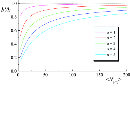
Figure 1: (Color online) The ratio $b^{\prime}/b$ as a function of the average number of projectile wounded nucleons $\langle N_{\rm proj}\rangle$ in Pb–Pb collisions for several values of the dispersion $\sigma$ of $N_{\rm proj}$. The most upper line corresponds to $\sigma=1$, the lower one to $\sigma=2$, etc.

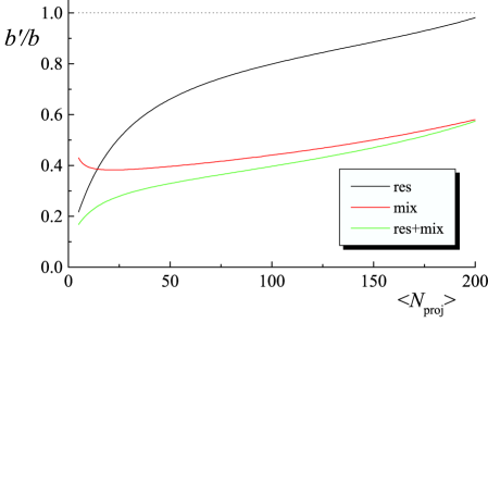
Figure 2: (Color online) $b^{\prime}/b$ vs. $\langle N_{\rm proj}\rangle$ in Pb–Pb collisions. The upper curve (‘res’) shows the effect of calorimeter resolution; the middle one (‘mix’) represents the mixing model; the lower curve (‘res+mix’) combines the effect of calorimeter resolution and the mixing-model prediction.

The dispersion of $N_{\rm proj}$ is usually not constant but it changes with $\langle N_{\rm proj}\rangle$. The energy resolution of the NA49 zero-degree calorimeter Rybczy which is recalculated into the dispersion of projectile participant number $N_{\rm proj}$ is

$$\sigma_{\rm proj}(\langle N_{\rm proj}\rangle)=0.77\sqrt{A-\langle N_{\rm proj}\rangle}-0.28-0.032\>(A-\langle N_{\rm proj}\rangle)\;,$$ (20)

where $A$ is the atomic number of the projectile nucleus. For the lead ($A=208$) projectile, the formula (20) gives $\sigma$ which varies only between 3.5 and 4.0 for $1<\langle N_{\rm proj}\rangle<150$, but it drops to 1.6 for $\langle N_{\rm proj}\rangle=200$. The prediction of the formula (19) with the dispersion of the wounded nucleon number given by Eq. (20) for $A=208$ is represented by the most upper curve labeled as ‘res’ in Fig. 2.

As mentioned in the Introduction, the transparency model, which assumes that the projectile participants mostly contribute to the particle production in the forward hemisphere, fails to describe Gazdzicki:2005rr ; Konchakovski:2005hq the large multiplicity fluctuations observed in the forward rapidity window Gazdzicki:2004ef ; Rybczynski:2004yw . The mixing models Gazdzicki:2005rr ; Konchakovski:2005hq , where the wounded nucleons from the projectile and target equally contribute to the forward rapidity window, agree, at least qualitatively, with the data Gazdzicki:2004ef ; Rybczynski:2004yw . So, let us consider the model predictions concerning the correlation $p_{T}$ vs. $N$. The average number of sources $\langle k\rangle$ then equals $(\langle N_{\rm proj}\rangle+\langle N_{\rm targ}\rangle)/2$ where $N_{\rm targ}$ is the number of wounded nucleons from the target nucleus. Since we consider collisions of identical nuclei $\langle N_{\rm targ}\rangle=\langle N_{\rm proj}\rangle$, and thus $\langle k\rangle=\langle N_{\rm proj}\rangle$.

We first neglect the experimental effect of finite calorimeter resolution, and we assume that $N_{\rm proj}$ is precisely determined - $N_{\rm proj}$ does not fluctuate and $\langle N_{\rm proj}\rangle=N_{\rm proj}$. The number of particle sources, which contribute to the forward hemisphere, fluctuates due to the fluctuations of $N_{\rm targ}$ at fixed $N_{\rm proj}$ and due to the collision dynamics: a wounded nucleon from the projectile (target) is assumed to contribute with probability 1/2 to the forward (backward) hemisphere. Then, the variance of the particle sources, which contribute to the forward hemisphere, is $\sigma^{2}=N_{\rm proj}/2+\sigma_{\rm targ}^{2}/4$, where $\sigma_{\rm targ}^{2}$ is the variance of $N_{\rm targ}$ at fixed $N_{\rm proj}$. Using the numerical results obtained within the Hadron-String Dynamics model Cassing:1999es , which were used in Gazdzicki:2005rr ; Konchakovski:2005hq , $\sigma_{\rm targ}^{2}$ can be roughly parameterized as

$$\sigma_{\rm targ}^{2}(N_{\rm proj})=3.28\>N_{\rm proj}-0.0158N_{\rm proj}^{2}\;,$$

for the Pb-Pb collisions. As seen, $\sigma_{\rm targ}$ vanishes for $N_{\rm proj}=0$ and $N_{\rm proj}=208$, and it reaches maximum equal 13.1 at $N_{\rm proj}=104$. Thus, the variance of the particle sources is

$$\sigma^{2}(N_{\rm proj})=1.32\>N_{\rm proj}-0.004N_{\rm proj}^{2}\;,$$ (21)

with maximum equal 10.4 at $N_{\rm proj}=165$. Substituting $\langle k\rangle=N_{\rm proj}$ and $\sigma$ given by Eq. (21) into the formula (19), one finds the result shown in Fig. 2 by the middle curve labeled as ‘mix’. As seen, the mixing model leads to a sizeable reduction of the correlation $p_{T}$ vs. $N$, and the reduction does not much depened on the collision centrality.

Finally, we have combined the effect of ‘mixing’ with that of the finite calorimeter resolution. Treating the two sources of fluctuations as independent from each other, the variances have been summed up. The result is shown in Fig. 2 by the lowest curve labeled as ‘res+mix’.

VI Summary and conclusions

The correlation $p_{T}$ vs. $N$, which is evident in p–p collisions, has been studied in the superposition model of nucleus–nucleus collisions where produced particles come from $k$ identical and independent sources. At first the number of sources has been treated as a fixed number, and then the fluctuations of $k$ have been taken into account. While the superposition of particle’s sources preserves the correlation strength, the correlation is strongly reduced by the source number fluctuations. The calculations are fully analytical.

The Wounded Nucleon Model has been used to formulate predictions for the NA49 measurement of the correlation $p_{T}$ vs. $N$ in Pb–Pb collisions. Since the measurement, which is underway, is performed in the forward rapidity window, it has been first assumed that only wounded nucleons from the projectile contribute there. Taking into account a finite energy resolution of the zero-degree calorimeter, which allows one to precisely fix the number of wounded nucleons from the projectile, the correlation has been found to be strongly reduced in the peripheral collisions while the reduction in the central collisions is quite small.

Then, the ‘mixed’ Wounded Nucleon Model Gazdzicki:2005rr ; Konchakovski:2005hq has been considered. The model, which appears to be successful in describing the multiplicity fluctuations at fixed number of the projectile wounded nucleons Gazdzicki:2004ef ; Rybczynski:2004yw , assumes, contrary to a natural expectation Bialas:2004su , that the wounded nucleons from the projectile and target equally contribute to the forward rapidity window. In this case, the correlation $p_{T}$ vs. $N$ seen in the forward rapidity window is strongly reduced and the reduction weakly depends on the collision centrality.

The correlation $p_{T}$ vs. $N$ seems to be responsible Mrowczynski:2004cg for the transverse momentum fluctuations Anticic:2003fd as quantified by the measure $\Phi(p_{T})$ Gazdzicki:ri . The data on the $p_{T}$ vs. $N$ correlation combined with the existing data on the multiplicity Gazdzicki:2004ef ; Rybczynski:2004yw and transverse momentum fluctuations Anticic:2003fd - all obtained in the same experimental conditions - will hopefully allow one to formulate a coherent picture of the event-by-event fluctuations observed in nucleus–nucleus collisions.

- (1) T. Kafka et al., Phys. Rev. D 16, 1261 (1977).
- (2) T. Antičić et al. [NA49 Collaboration], Phys. Rev. C 70, 034902 (2004).
- (3) M. Gaździcki and St. Mrówczyński, Z. Phys. C 54, 127 (1992).
- (4) St. Mrówczyński, M. Rybczyński and Z. Włodarczyk, Phys. Rev. C 70, 054906 (2004).
- (5) M. Gaździcki et al. [NA49 Collaboration], J. Phys. G 30, S701 (2004).
- (6) M. Rybczyński et al. [NA49 Collaboration], J. Phys. Conf. Ser. 5, 74 (2005).
- (7) A. Białas, M. Błeszyński and W. Czyż, Nucl. Phys. B 111, 461 (1976).
- (8) M. Gaździcki and M. Gorenstein, arXiv:hep-ph/0511058.
- (9) V. P. Konchakovski, S. Haussler, M. I. Gorenstein, E. L. Bratkovskaya, M. Bleicher and H. Stöcker, Phys. Rev. C 73, 034902 (2006).
- (10) A. Wróblewski, Acta Phys. Polon. B 4, 857 (1973).
- (11) M. Rybczyński, Ph.D. thesis, Kielce, 2005.
- (12) A. Białas and W. Czyż, Acta Phys. Polon. B 36, 905 (2005).
- (13) W. Cassing and E. L. Bratkovskaya, Phys. Rept. 308, 65 (1999).