Exact Solution of the Isovector Proton Neutron Pairing Hamiltonian

Abstract

The complete exact solution of the $T=1$ neutron-proton pairing Hamiltonian is presented in the context of the SO(5) Richardson-Gaudin model with non-degenerate single-particle levels and including isospin-symmetry breaking terms. The power of the method is illustrated with a numerical calculation for ⁶⁴Ge for a $pf+g_{9/2}$ model space which is out of reach of modern shell-model codes.

Exactly solvable models (ESM) provide important insights into the structure of many-body quantum systems. The two main advantages of ESMs are: (1) They can describe in an analytical or exact numerical way a wide variety of elementary phenomena. (2) They can be and have been used as a testing ground for various many-body approaches.

A particular class of ESMs, extensively used in nuclear physics, are the dynamical-symmetry models. In this case the Hamiltonian can be expressed in terms of Casimir operators of a chain of nested algebras. An example often used to introduce nuclear superconductivity (see e.g. Ref. Rin80 ) is the rank-1 (Lie) algebra SU(2). Examples of dynamical-symmetry models associated with a rank-2 algebra are Elliott’s SU(3) model of nuclear deformation Ell58 and the SO(5) model of $T=1$ isovector pairing between neutrons and protons Flo52 which has found many applications in nuclei (see e.g. Ref. so5 ).

The concept of quantum integrability, closely linked with exact solvability, goes beyond the limits of the dynamical-symmetry approach. A quantum system is integrable if there exist as many commuting Hermitian operators (integrals of motion) as quantum degrees of freedom Zha95 . The set of Casimir operators of a chain of nested algebras satisfies this condition.

Dynamical-symmetry models are usually defined for degenerate single-particle levels. Lifting this degeneracy breaks the dynamical symmetry but may still preserve integrability. The pairing model with non-degenerate single-particle levels, of which an exact solution was found by Richardson in the sixties Ric63 , represents an example of an ESM with such characteristics. Recently, more general exactly solvable pairing models, both for fermions and for bosons, called Richardson-Gaudin (RG) models, have been proposed Duk01 ; Duk04 .

The RG pairing models are based on rank-1 algebras: SU(2) for fermions and SU(1,1) for bosons. In this Letter we carry out the first step in extending the RG models to higher-rank algebras by considering a RG model based on the rank-2 algebra SO(5). The model Hamiltonian describes a two-component system consisting of neutrons and protons interacting through an isovector ($T=1$) pairing force and distributed over non-degenerate orbits. This neutron-proton (np) pairing Hamiltonian with non-degenerate orbits has been studied by Richardson Ric66 who proposed an exact solution. However, it was shown subsequently that Richardson’s solution is incorrect for more than two nucleon pairs Pan02 by explicitly solving the case of three-nucleon pairs. Independently, Links et al. derived an exact solution for the isospin invariant SO(5) model by making use of the quantum inverse scattering method Lin02 .

We present here the most general exact solution of the RG SO(5) model including isospin symmetry breaking terms and for states with arbitray seniority. In addition to the construction of the complete set of integrals of motion from which more general exactly solvable pn-pairing Hamiltonians can be derived, we present here the first numerical exact solution of the SO(5) RG model for ⁶⁴Ge in a Hilbert space built from the $pf+g_{9/2}$ shells, of which the dimension goes well beyond the limits of modern shell-model codes based on exact diagonalization.

SO(5) has also been proposed as the symmetry underlying high-$T_{\rm c}$ superconductivity Dem04 . The exactly solvable RG model discussed in this Letter may conceivably be used to generalize SO(5) condensed-matter models Wu03 by the explicit addition of non-degenerate single-particle symmetry-breaking terms. Other possible applications might be found in polarized ultracold Fermi gases with $p$-wave pairing interactions Gu .

We begin by introducing the 10 generators of the SO(5) algebra in a representation well suited for nuclear physics problems. Let us define first the three $T=1$ pair-creation operators: $\hat{b}^{\dagger}_{-1,i}=\hat{n}_{i}^{\dagger}\hat{n}_{\bar{\imath}}^{\dagger}$, $\hat{b}^{\dagger}_{0,i}=(\hat{n}_{i}^{\dagger}\hat{p}_{\bar{\imath}}^{\dagger}+\hat{p}_{i}^{\dagger}\hat{n}_{\bar{\imath}}^{\dagger})/\sqrt{2}$, and $\hat{b}^{\dagger}_{+1,i}=\hat{p}_{i}^{\dagger}\hat{p}_{\bar{\imath}}^{\dagger}$, where $n$ and $p$ refer to neutrons and protons, respectively, and $i$ labels a single-particle basis (with ${\bar{\imath}}$ its time-reversed state) which may be associated with the spherical shell-model basis $i\equiv jm$ or with an axially-symmetric deformed basis $i\equiv\alpha m$. The three pair-annihilation operators are $\hat{b}_{-1,i}$, $\hat{b}_{0,i}$, and $\hat{b}_{+1,i}$. The three components of the isospin operator [$\hat{T}_{+,i}=(\hat{p}_{i}^{\dagger}\hat{n}_{i}+\hat{p}_{\bar{\imath}}^{\dagger}\hat{n}_{\bar{\imath}})/\sqrt{2}$, $\hat{T}_{0,i}=(\hat{p}_{i}^{\dagger}\hat{p}_{i}+\hat{p}_{\bar{\imath}}^{\dagger}\hat{p}_{\bar{\imath}})/2-(\hat{n}_{i}^{\dagger}\hat{n}_{i}+\hat{n}_{\bar{\imath}}^{\dagger}\hat{n}_{\bar{\imath}})/2$, and $\hat{T}_{-,i}=(\hat{n}_{i}^{\dagger}\hat{p}_{i}+\hat{n}_{\bar{\imath}}^{\dagger}\hat{p}_{\bar{\imath}})/\sqrt{2}$] close the ${\rm SU}_{T}(2)$ subalgebra of SO(5). These 9 operators together with the number operator $\hat{N}_{i}=\hat{p}_{i}^{\dagger}\hat{p}_{i}+\hat{p}_{\bar{\imath}}^{\dagger}\hat{p}_{\bar{\imath}}+\hat{n}_{i}^{\dagger}\hat{n}_{i}+\hat{n}_{\bar{\imath}}^{\dagger}\hat{n}_{\bar{\imath}}$ define the SO(5) algebra.

For a system with $L$ single-particle states $i=1,...,L$ there are $L$ integrals of motion:

$$\hat{R}_{i} = (2+\Delta)\hat{H}_{i}+\Delta\hat{T}_{0,i}+2g\sum_{i^{\prime}(\neq i)=1}^{L}\frac{1}{z_{i}-z_{i^{\prime}}}$$

$$\times \left[\sum_{\mu}\left(\hat{b}_{\mu,i}^{\dagger}\hat{b}_{\mu,i^{\prime}}+\hat{b}_{\mu,i^{\prime}}^{\dagger}\hat{b}_{\mu,i}\right)+\hat{T}_{i}\cdot\hat{T}_{i^{\prime}}+\hat{H}_{i}\hat{H}_{i^{\prime}}\right],$$

where $\hat{H}_{i}=\hat{N}_{i}/2-1$. The expression (Exact Solution of the Isovector Proton Neutron Pairing Hamiltonian) follows from the integrals of motion valid for any semi-simple algebra of arbitrary rank Aso02 . Since SO(5) is of rank 2, its Cartan subalgebra contains two elements namely $\hat{H}_{i}$ and $\hat{T}_{0,i}$ in the chosen basis which therefore appear linearly in (Exact Solution of the Isovector Proton Neutron Pairing Hamiltonian). The set of $L$ parameters $z_{i}$ together with the two constants $g$ and $\Delta$ can be freely chosen and it is straightforward to check that the integrability condition $[\hat{R}_{i},\hat{R}_{j}]=0$ is valid for any choice of the $L+2$ parameters. A simplified version of (Exact Solution of the Isovector Proton Neutron Pairing Hamiltonian) was previously derived using the algebraic Bethe ansatz Lin02 .

The eigenvalues of the integrals of motion are

$$r_{i} = 2g\!\!\!\!\!\!\sum_{i^{\prime}(\neq i)=1}^{L}\frac{\left(\frac{v_{i}}{2}-1\right)\left(\frac{v_{i^{\prime}}}{2}-1\right)+t_{i}t_{i^{\prime}}}{z_{i}-z_{i^{\prime}}}-g\!\!\!\!\!\!\sum_{\beta=1}^{M+T_{0}+t}\frac{2t_{i}}{z_{i}-\omega_{\beta}}$$ (2)

$$+ g\sum_{\alpha=1}^{M}\frac{v_{i}+2t_{i}-2}{z_{i}-e_{\alpha}}+\left[(2+\Delta)\left(\frac{v_{i}}{2}-1\right)-\Delta t_{i}\right]\!,$$

where $e_{\alpha}$ and $\omega_{\beta}$ are solutions of the equations

$$\frac{1}{g} = \frac{1}{2}\sum_{i=1}^{L}\frac{v_{i}+2t_{i}-2}{z_{i}-e_{\alpha}}+\sum_{\alpha^{\prime}(\neq\alpha)=1}^{M}\frac{2}{e_{\alpha^{\prime}}-e_{\alpha}}$$ (3)

$$- \sum_{\beta=1}^{M+T_{0}+t}\frac{1}{\omega_{\beta}-e_{\alpha}},$$

$$\frac{\Delta}{g} = \sum_{\beta^{\prime}(\neq\beta)=1}^{M+T_{0}+t}\frac{2}{\omega_{\beta^{\prime}}-\omega_{\beta}}-\sum_{\alpha=1}^{M}\frac{2}{e_{\alpha}-\omega_{\beta}}-\sum_{i=1}^{L}\frac{2t_{i}}{z_{i}-\omega_{\beta}}.$$

The meaning of the quantum numbers appearing in (2) and (3) is as follows: $v_{i}$ is the seniority of each $i$ level, i.e. the number of fermions not paired in time-reversed states with isospin $T=1$, $t_{i}$ is the isospin of the unpaired fermions (this quantum number is often called reduced isospin Hec65 ), $t=\sum_{i}t_{i}$, $M$ is the number of $T=1$ time-reversed pairs, and $T_{0}$ is the $z$ component of the total isospin, i.e. the eigenvalue of the operator $\hat{T}_{0}=\sum_{i}\hat{T}_{0,i}$. The total number of nucleons is $N=N_{p}+N_{n}=2M+\sum_{i}v_{i}$ whereas their difference is $N_{p}-N_{n}=2T_{0}$. The quantum numbers $M$, $T_{0}$, $v_{i}$, and $t_{i}$ are conserved; $T$ is also conserved if $\Delta=0$.

Although any function of the $\hat{R}_{i}$ can be used as an integrable Hamiltonian, the linear combination $\sum_{i=1}^{L}z_{i}\hat{R}_{i}$ yields simple expressions for the np-pairing Hamiltonian and its corresponding eigenvalues:

$$\hat{H} = \frac{1}{2}\sum_{i=1}^{L}z_{i}\hat{R}_{i}+g\hat{C}$$

$$= \sum_{j}\varepsilon_{j}\left(\hat{N}_{j}+\Delta\hat{N}_{p,j}\right)+\frac{g}{2}\hat{T}\cdot\hat{T}+g\!\!\!\!\sum_{\mu jmj^{\prime}m^{\prime}}\!\!\!\hat{b}_{\mu,jm}^{\dagger}\hat{b}_{\mu,j^{\prime}m^{\prime}},$$

where $\hat{C}$ is a constant operator depending on the conserved quantities. We have introduced the variables $\varepsilon_{j}=z_{j}/2$ and specialized to a spherical basis $i\equiv jm$. The second term on the r.h.s. of (Exact Solution of the Isovector Proton Neutron Pairing Hamiltonian) breaks the isospin symmetry. For $\Delta\neq 0$ the operator $\hat{T}^{2}$ does not commute with the Hamiltonian (Exact Solution of the Isovector Proton Neutron Pairing Hamiltonian) and, consequently, $T$ is not a good quantum number but $T_{0}$ is still a conserved quantity. The same linear combination of the $r_{i}$ and the use of the Richardson equations (3), yield the eigenvalues of (Exact Solution of the Isovector Proton Neutron Pairing Hamiltonian):

$$E = \sum_{\alpha=1}^{M}e_{\alpha}+\frac{\Delta}{2}\!\sum_{\beta=1}^{M+T_{0}+t}\!w_{\beta}+\sum_{j}\varepsilon_{j}\left[\frac{v_{j}}{2}(2+\Delta)-\Delta t_{j}\right]$$ (5)

$$+\frac{g}{2}T_{0}(T_{0}-1).$$

Each solution of the equations (3) gives an eigenstate of the np-pairing Hamiltonian. The spectral parameters $e_{\alpha}$ are interpreted as pair energies as in the case of SU(2) pairing. However, due to the larger rank of SO(5), a new set of spectral parameters $w_{\beta}$ appears in the equations (3). These new parameters are associated with the ${\rm SU}_{T}(2)$ isospin subalgebra and there are $M+T_{0}+t$ of them. In the limit $\Delta=0$ the number of finite $w_{\beta}$ parameters reduces to $M+t-T$ for each possible isospin $T$. The Bethe ansatz for the SO(5) eigenstates of the RG model is a product wave function Ush94 :

$$\left(\prod\limits_{\alpha=1}^{M}\hat{b}_{-1}^{\dagger}(e_{\alpha})\right)\prod\limits_{\beta=1}^{M+T_{0}+t}\left(\hat{T}_{+}(w_{\beta})-\sum_{\alpha=1}^{M}\frac{\hat{I}_{+,\alpha}}{w_{\beta}-e_{\alpha}}\right)|\Lambda\rangle,$$ (6)

where the spectral dependence of the operators is

$$\hat{T}_{+}(w_{\beta})=\ \sum_{i}\frac{\hat{T}_{+,i}}{2\varepsilon_{i}-w_{\beta}},\quad\hat{b}_{\mu}^{\dagger}(e_{\alpha})=\sum_{i}\frac{\hat{b}^{\dagger}_{\mu,i}}{2\varepsilon_{i}-e_{\alpha}},$$ (7)

and $\hat{I}_{+,\alpha}$ is a raising operator for $\hat{b}_{\mu}^{\dagger}(e_{\alpha})$: $\hat{b}_{\mu}^{\dagger}(e_{\alpha})\hat{I}_{+,\alpha}=\hat{b}_{\mu+1}^{\dagger}(e_{\alpha})$ for $\mu=-1,0$, $\hat{b}_{+1}^{\dagger}(e_{\alpha})\hat{I}_{+,\alpha}=0$, and $|\Lambda\rangle$ is a lowest-weight state defined by $\hat{b}_{\mu,i}|\Lambda\rangle=\hat{T}_{-,i}|\Lambda\rangle=0$. To show the behavior of the spectral parameters $e_{\alpha}$ and $\omega_{\beta}$ as a function of the isospin-breaking term $\Delta$, we plot in Fig. 1 some selected solutions of the Richardson equations (3) for a system of two neutrons and two protons in two shells ($j_{0}=1/2$ and $j_{1}=3/2$) within the seniority-0 subspace ($M=2,T_{0}=0,t_{i}=v_{i}=0$).

Figure 1: Pair energies $e_{\alpha}$ (dashed lines) and spectral parameters $\omega_{\beta}$ (solid lines) as a function of the parameter $\Delta$ for three different states of a 2n-2p system with two shells ($j_{0}=1/2$ and $j_{1}=3/2$) in the seniority-0 subspace. The label $T$ refers to the isospin in the limit $\Delta=0$. The figure shows the lowest-energy states of the Hamiltonian (Exact Solution of the Isovector Proton Neutron Pairing Hamiltonian) for each $T$ with energies plotted in the bottom-right panel. Since the spectral parameters of the $T=1$ state are real, their imaginary part is not shown. The interaction strength and single-particle energies are $g=-1$, $\varepsilon_{0}=0$, and $\varepsilon_{1}=1$.

For $\Delta=0$ there are two finite $\omega_{\beta}$ complex conjugate parameters for $T=0$ while the two pair energies are real and negative, for $T=1$ there is one real, finite $\omega_{\beta}$ and two real pair energies $e_{\alpha}$, and, finally, the $T=2$ case reduces to SU(2) for like particles with two $e_{\alpha}$ parameters forming a complex conjugate pair. For finite $\Delta$ there is isospin mixing and the number of finite parameters $\omega_{\beta}$ is always two. Figure 1 thus confirms that the number of finite $\omega_{\beta}$ spectral parameters reduces from $M=2$ to $M-T$ when $\Delta\rightarrow 0$. For $T=1$ one of the real $\omega_{\beta}$ goes to $-\infty$ in this limit, vanishing from the Richardson equations (3) but giving a finite contribution to the Hamiltonian eigenvalues (Exact Solution of the Isovector Proton Neutron Pairing Hamiltonian) note . Analogously, in the $T=2$ case the two $\omega$ parameters tend to $\infty$ in the $\Delta=0$ limit. Also shown are the energies of the three eigenstates of the np-pairing Hamiltonian (Exact Solution of the Isovector Proton Neutron Pairing Hamiltonian). We emphasize that, while these are the eigenvalues of a particular Hamiltonian, the spectral parameters completely define the eigenfunction (6) of the $L$ integrals of motion (Exact Solution of the Isovector Proton Neutron Pairing Hamiltonian) from which $\hat{H}$ is constructed and their corresponding eigenvalues (2).

We now turn to the discussion of a numerical calculation for ⁶⁴Ge. We consider a model space that is well beyond modern shell-model capabilities based on exact diagonalization: 12 valence neutrons and 12 valence protons with a ⁴⁰Ca core. The adopted single-particle energies are (in MeV) $\varepsilon_{f_{7/2}}=0.00$, $\varepsilon_{p_{3/2}}=6.00$, $\varepsilon_{f_{5/2}}=6.25$, $\varepsilon_{p_{1/2}}=7.1$, and $\varepsilon_{g_{9/2}}=9.60$, and two pairing strengths, $g=-0.05$ (weak) and $-0.5$ (strong), are considered. We assume isospin symmetry ($\Delta=0$) and consider the seniority-0 subspace.

Results for the lowest $T=0$, 1, and 2 states are shown in Fig. 2.

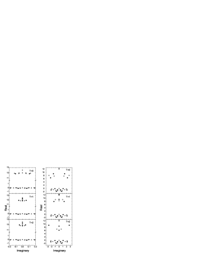
Figure 2: Complex-plane representation of the pair energies $e_{\alpha}$ and spectral parameters $\omega_{\beta}$ for the lowest-energy states with isospin $T=0,1,2$ in ⁶⁴Ge. The left panel corresponds to weak coupling $g=-0.05$ and the right panel to strong coupling $g=-0.5$. The squares represent the three lowest single-particle energies ($2\varepsilon_{f_{7/2}}=0.00$, $2\varepsilon_{p_{3/2}}=12$, $2\varepsilon_{f_{5/2}}=12.5$), the black circles are the pair energies $e_{\alpha}$, and the grey circles are the parameters $\omega_{\beta}$. All energies are in MeV.

The $T=0$ solution corresponds to the ground state while the $T=1$ and $T=2$ solutions are excited states in ⁶⁴Ge. As in SU(2), the different configurations can be classified in the weak-coupling limit. At weak coupling ($g\rightarrow 0$) eight pairs occupy the $f_{7/2}$ level and four pairs are in the $p_{3/2}$ level for the state with $T=0$. This is reflected in the upper left panel of figure 2 where 8 pair energies appear close to $2\varepsilon_{f_{7/2}}$ and 4 pair energies are close to $2\varepsilon_{p_{3/2}}$ making the corresponding terms in (7) dominant. Due to the Pauli principle, this configuration is not allowed for a state with $T=1$ and, correspondingly, one pair energy is close to $2\varepsilon_{f_{5/2}}$. In all cases the $w_{\beta}$ parameters are intertwined with the pair energies $e_{\alpha}$. The number of $w_{\beta}$ parameters ($M-T$), together with the initial configuration at weak coupling, defines each eigenstate of the np-pairing Hamiltonian. As $|g|$ increases, the $e_{\alpha}$ and $w_{\beta}$ parameters expand in the complex plain. The solutions are subject to numerical instabilities due to singularities arising when a real pair energy $e_{\alpha}$ crosses a single-particle energy or when real $e_{\alpha}$ and $w_{\beta}$ parameters cross. An example of the first class of crossings can be observed in Fig. 2 for $T=2$ where the pair energy above the $p_{3/2}$ level at weak coupling goes down with increasing $g$ and crosses the $p_{3/2}$ single-particle energy. The $T=1$ case shows an exchange of positions on the real axis of a pair energy $e_{\alpha}$ and a $w_{\beta}$ parameter as an example of the second class of singularities. The first class of singularities was already present in SU(2) pairing and precluded the practical use of Richardson’s solution for a long time. Recently, a new method to overcome this numerical problem was proposed Rom04 . We believe that the same procedure can be used to treat the second class of singularities as well, allowing the exact solution of the SO(5) model for very large systems.

As a further illustration of the method we show in Fig. 3 the eigenenergies and the occupation probablities of single-particle levels as a function the pairing strength.

Figure 3: Eigenenergies and occupation probablities of single-particle levels of the $T=0$, 1, and 2 states in ⁶⁴Ge as a function of the pairing strength $g$.

The occupation probabilities can be obtained making use of Hellmann-Feynman theorem which expresses them in terms of derivatives of the eigenvalues of the integrals of motion $r_{i}$ as $\langle N_{p,i}\rangle=1+\frac{\partial r_{i}}{\partial\Delta}$, and $\langle N_{n,i}\rangle=r_{i}-g\frac{\partial r_{i}}{\partial g}-(1+\Delta)\left(1+\frac{\partial r_{i}}{\partial\Delta}\right)+1$. These derivatives can be related to the derivatives of the spectral parameters $e_{\alpha}$ and $\omega_{\alpha}$, which in turn can be obtained taking the derivatives of the Richardson equations (3).

In summary, as an application of generalized RG models, we have presented the complete solution of the SO(5) isovector np-pairing problem. The generalization allows the introduction of one-body symmetry-breaking terms, such as non-degenerate single-particle energies, yielding an exact solution of the SO(5) np-pairing model for arbitrary seniorities even if it includes an isospin-breaking term. The numerical solution of the SO(5) Richardson equations was presented for the specific example of ⁶⁴Ge, together with a discussion of the behavior of the spectral parameters for weak and strong pairing. With this work the exact solution for large systems with SO(5) symmetry is now available which could be of great importance in condensed-matter physics when addressing the phenomenon of high-$T_{\rm c}$ superconductivity Dem04 ; Wu03 . Finally, the treatment of higher-rank algebras like Sp(6) and SO(8) opens the possibility of exact nuclear structure calculations with more realistic quantum integrable models.

This work was supported in part by the Spanish DGI under grant No. BFM2003-05316-C02-02, by Bulgarian contracts $\Phi-1416$ and $\Phi-1501$ and by a CICYT-IN2P3 cooperation. V.G.G. acknowledges financial support from a NATO fellowship and from the US DOE under grant No. W-7405-Eng-48. S.L.H. has a post-doctoral fellowship from the Spanish SEUI-MEC and B.E. has a pre-doctoral grant from the Spanish CE-CAM.

References

- (1) P. Ring and P. Schuck, The nuclear many body problem (Springer-Verlag, New York, 1980).
- (2) J. P. Elliott, Proc. Roy. Soc. A 245, 128 (1958); 245, 562 (1958).
- (3) B.H. Flowers, Proc. Roy. Soc. A 212, 248 (1952).
- (4) J. Engel, K. Langanke, and P. Vogel, Phys. Lett. B 389, 211 (1996).
- (5) W.M. Zhang and D.H. Feng, Phys. Rep. 252, 1 (1995).
- (6) R.W. Richardson, Phys. Lett. 3, 277 (1963); Phys. Rev. 141, 949 (1966).
- (7) J. Dukelsky, C. Esebbag, and P. Schuck, Phys. Rev. Lett. 87, 066403 (2001).
- (8) J. Dukelsky, S. Pittel, and G. Sierra, Rev. Mod. Phys. 76, 643 (2004).
- (9) R.W. Richardson, Phys. Rev. 144, 874 (1966).
- (10) F. Pan and J.P. Draayer, Phys. Rev. C 66, 044314 (2002).
- (11) M. Asorey, F. Falceto, and G. Sierra, Nucl. Phys. B 622, 593 (2002).
- (12) J. Links, H.-Q. Zhou, M.D. Gould, and R.H. McKenzie, J. Phys. A 35, 6459 (2002).
- (13) E. Demler, W. Hanke, and S.-C. Zhang, to be published in Rev. Mod. Phys. cond-mat/0405038.
- (14) L.-A. Wu, M. Guidry, Y. Sun, and C.-L. Wu, Phys. Rev. B 67, 014515 (2003).
- (15) V. Gurarie, L. Radzihovsky, and A. V. Andreev, Phys. Rev. Lett. 94, 230403 (2005).
- (16) It can be shown that in the limit the second term for the diverging and the fourth term in (5) combine to give .
- (17) K.T. Hecht, Phys. Rev. 139, B794 (1965).
- (18) A.G. Ushveridize, Quasi-exactly solvable models in quantum mechanics (Institute of Physics, Bristol and Philadelphia, 1994).
- (19) S. Rombouts, D. Van Neck, and J. Dukelsky, Phys. Rev. C 69, 060303 (2004).