Ground state of medium-heavy doubly-closed shell nuclei
in correlated basis function theory

Abstract

The correlated basis function theory is applied to the study of medium-heavy doubly closed shell nuclei with different wave functions for protons and neutrons and in the $jj$ coupling scheme. State dependent correlations including tensor correlations are used. Realistic two-body interactions of Argonne and Urbana type, together with three-body interactions have been used to calculate ground state energies and density distributions of the ¹²C , ¹⁶O , ⁴⁰Ca , ⁴⁸Ca and ²⁰⁸Pb nuclei.

I INTRODUCTION

In the last decade, the validity of the non relativistic many-body theory in the description of nuclear systems, has been well established. The idea is to describe the nucleus as a set of mutually interacting nucleons with a hamiltonian of the type

$$H=\sum_{i}\frac{-\hbar^{2}}{2m_{i}}\nabla^{2}_{i}+\sum_{i<j}v_{ij}+\sum_{i<j<k}v_{ijk}$$ (1)

where the two- and three-body interactions, $v_{ij}$ and $v_{ijk}$ respectively, are fixed to reproduce the properties of the two- and three-body systems.

Quantum Monte Carlo calculations solve the many-body Schrödinger equation without approximations Pudliner et al. (1995, 1997) and have been applied with success to describe nuclei up to twelve nucleons Pieper (2005). The only limitation of this approach is related to the available computing power, which, at present, does not allow its straightforward application to medium and heavy nuclei. The good results obtained by the Quantum Monte Carlo calculations have renewed the interest in nuclear structure calculations with realistic, or microscopic, interactions. For this reason, many-body techniques, which are not approximation free, have been formulated, or reconsidered, and applied to the study of medium and heavy nuclei, or more in general, to nuclear systems with A$>$4.

The oldest, and most commonly used, technique is the Brueckner Hartree-Fock approach recently applied to calculate the properties of ¹⁶O Schmid et al. (1991); Dickhoff and Barbieri (2004). In the last years, no-core shell model calculations Navrátil et al. (2000); Forssén et al. (2005) have used microscopic interactions to calculate some property of nuclei up to ¹²C . The coupled cluster method has been used to evaluate ¹⁶O properties Heisenberg and Mihaila (1999); Mihaila and Heisenberg (1999); Dean and al. (2005). More recently a technique called Unitary Correlation Operator Method has been developed to produce effective interactions used in mean-field and shell model calculations, and it has been applied with success to a variety of nuclei up to ²⁰⁸Pb Neff and Feldmeier (2003); Roth et al. (2004).

In the early nineties, we started a project aimed to apply to finite nuclei the Correlated Basis Function (CBF) theory, originally developed for infinite systems Rosati (1982). The idea was to use the Fermi Hypernetted Chain (FHNC) resummation technique, well tested in nuclear matter, to describe finite systems. We first tested the validity of our approach in model nuclei with degenerate proton and neutron states, and in $ls$ coupling scheme Co’ et al. (1992, 1994). Then, by using central interactions and scalar correlation functions, we applied the theory to describe nuclei with different single particle bases for protons and neutrons, with different number of protons and neutrons and with the more realistic $jj$ coupling scheme de Saavedra et al. (1996). More recently, we have treated two-body interactions containing tensor and spin-orbit terms and this implies the use of state dependent correlations Fabrocini et al. (1998). This was not a straightforward extension of the formalism because the non commutativity of the different operators requires the use of the Single Operator Chain (SOC) approximation in the FHNC resummation. The FHNC/SOC computational scheme has been extended to include spin-orbit and three-body interactions of Urbana and Argonne type Fabrocini et al. (2000). In these last calculations protons and neutrons single particle wave functions were distinguished only by the third component of the isospin, and they were treated in the $ls$ coupling scheme. This choice allowed us to treat only systems saturated in spin and isospin.

This paper represents a step forward in our project. The FHNC/SOC formalism has been extended to treat nuclei with different proton and neutrons wave functions, and in a $jj$ coupling scheme in spherical basis. With this single particle basis we obtained results for the ¹²C , ¹⁶O , ⁴⁰Ca , ⁴⁸Ca and ²⁰⁸Pb nuclei.

The aim of this paper is to present the results we have obtained by using the two-body Argonne $v^{\prime}_{8}$ Wiringa et al. (1995); Pudliner et al. (1997) and the Urbana $v_{14}$ Lagaris and Pandharipande (1981a, b) interactions, where we have considered all the channels up to the spin-orbit ones. In our calculations we have implemented these two-body interactions with the Urbana IX Pudliner et al. (1997) and the Urbana VII Schiavilla et al. (1986) three-body interactions respectively.

In Sect. II we briefly discuss the basic ideas of the formalism pointing out the main differences with respect to what has been presented in Fabrocini et al. (1998) and Fabrocini et al. (2000). The detailed presentation of the heavy formalism, which is given in Bisconti (2005), is beyond the scope of this article.

II THE FORMALISM

Our approach is based on the variational principle, i.e. we search for the minimum of the energy functional

$$E[\Psi]=\frac{<\Psi|H|\Psi>}{<\Psi|\Psi>}$$ (2)

We used the hamiltonian of eq. (1) in our calculations, and we express the two-body interaction in the form

$$v_{ij}=\sum_{p=1,8}v_{p}(r_{ij})O^{p}_{ij}$$ (3)

where we have defined the operators $O^{p}$ as:

$$O^{p=1,8}_{ij}=[1,\mbox{\boldmath$\sigma$}_{i}\cdot\mbox{\boldmath$\sigma$}_{j},S_{ij},({\bf L}\cdot{\bf S})_{ij}]\otimes[1,\mbox{\boldmath$\tau$}_{i}\cdot\mbox{\boldmath$\tau$}_{j}]$$ (4)

and where we have indicated with $S_{ij}$ the tensor operator

$$S_{ij}=3\frac{{\bf r}_{ij}\cdot\mbox{\boldmath$\sigma$}_{i}{\bf r}_{ij}\cdot\mbox{\boldmath$\sigma$}_{j}}{r^{2}_{ij}}-\mbox{\boldmath$\sigma$}_{i}\cdot\mbox{\boldmath$\sigma$}_{j}$$ (5)

In eq. (3) we have limited the sum to the first 8 channels which are those used in our calculations. In reality modern two-body interactions have been parametrized by using up to 18 different channels Wiringa et al. (1995).

The three-body interaction Pudliner et al. (1997); Schiavilla et al. (1986) is composed by two parts. A first one describes the process where two pions are exchanged with the intermediate excitation of a $\Delta$ Fujita and Miyazawa (1957). This term describes the long-range part of the three-body interaction and, usually, gives an attractive contribution. The second part of the three-body interaction is a shorter range, repulsive, spin and isospin independent term. This term is supposed to simulate dispersive effects obtained when the $\Delta$ degrees of freedom are integrated out.

The search for the energy minimum (2) is done in the subspace of the many-body wave functions $\Psi$ which can be expressed as:

$$\Psi(1,2,...,A)=F(1,2,...,A)\Phi(1,2,....,A)$$ (6)

where $F(1,2,...,A)$ is a many-body correlation function and $\Phi(1,2,....,A)$ is a Slater determinant composed by a set of single particle wave functions $\phi_{\alpha}(i)$. In our calculations we describe the many-body correlation function as a symmetrized product of two-body correlation functions:

$$F(1,2,...,A)={\mathcal{S}}\left[\prod_{i<j}F_{ij}\right]$$ (7)

and we use two-body correlation functions $F_{ij}$ which have an operator dependence analogous to that of the nucleon-nucleon interaction (3), but without the spin-orbit terms:

$$F_{ij}=\sum_{p=1,6}f_{p}(r_{ij})O^{p}_{ij}$$ (8)

II.1 The cluster expansion

The evaluation of the multidimensional integrals necessary to calculate the energy functional (2) is done by performing a cluster expansion and by applying the FHNC resummation techniques. Our work is based on the formalism developed in Pandharipande and Wiringa (1979); Co’ et al. (1992); de Saavedra et al. (1996); Fabrocini et al. (1998).

The two basic quantities used in the cluster expansion of eq. (2) are the one- and the two-body density matrices respectively defined as:

$$\rho_{1}(x_{1},x^{\prime}_{1}) = A\int dx_{2}\,dx_{3}...dx_{A}\,\Psi^{*}(x_{1},x_{2},...,x_{A})\Psi(x^{\prime}_{1},x_{2},...,x_{A})/<\Psi|\Psi>$$ (9)

$$\rho_{2}(x_{1},x_{2}) = A(A-1)\int dx_{3}...dx_{A}\,\Psi^{*}(x_{1},x_{2},x_{3},...,x_{A})\Psi(x_{1},x_{2},x_{3},...,x_{A})/<\Psi|\Psi>$$ (10)

where we have indicate with $x_{i}$ the coordinate fully characterizing the particle $i$, i.e. position ${\bf r}_{i}$, 3-rd components of the spin, $s$, and of the isospin, $t$. The evaluation of the expectation values of one- and two-body operators can be obtained by making the operators acting on the densities (9) and (10) and integrating on the free variables.

In the uncorrelated case, $F(1,2,...,A)=1$, the expressions (9) and (10) become:

$$\rho^{o}_{1}(x_{1},x^{\prime}_{1}) = \sum_{i}\phi^{*}_{i}(x_{1})\phi_{i}(x^{\prime}_{1})$$ (11)

$$\rho^{o}_{2}(x_{1},x_{2}) = \rho^{o}_{1}(x_{1})\rho^{o}_{1}(x_{2})-\rho^{o}_{1}(x_{1},x_{2})\rho^{o}_{1}(x_{2},x_{1})$$ (12)

where we have indicated with $\phi_{i}$ the single particle wave functions. In the above equations, the sum is done on all the occupied states, and we have used the notation $\rho^{o}_{1}(x_{1})\equiv\rho^{o}_{1}(x_{1},x_{1})$ to indicate the diagonal part of the one-body density function.

We construct the single particle wave functions by using a spherical mean field potential containing a spin-orbit term. Protons and neutrons wave functions are generated by different potentials. The single particle wave functions are classified in terms of the angular momentum $j$ and of the third component of the isospin $t$. They can be written as:

$$\phi^{t}_{nljm}({\bf r}_{i})=R^{t}_{nlj}(r_{i})\sum_{\mu,s}<l\mu\frac{1}{2}s|jm>Y_{l\mu}(\Omega_{i})\chi_{s}(i)\chi_{t}(i)$$ (13)

where we have indicated with $Y_{l\mu}(\Omega_{i})$ the spherical harmonics, with $\chi_{s,t}(i)$ the Pauli spinor/isospinor and with $<l\mu\frac{1}{2}s|jm>$ the Clebsch-Gordan coefficient.

In the calculations of Refs. Co’ et al. (1992); Fabrocini et al. (1998, 2000), the radial part of the single particle wave function was independent on the isospin. This, joined to the fact that we studied doubly closed shell nuclei on $ls$ coupling with the same number of protons and neutrons, allowed us to separate the spatial part from the spin and isospin dependent parts in $\rho^{o}_{1}(x_{1},x^{\prime}_{1})$. Because we restricted our investigation to finite systems saturated in spin and isospin, we could use the trace techniques developed in Pandharipande and Wiringa (1979) to deal with state dependent correlations.

In the present case, as pointed out in de Saavedra et al. (1996), the choice of the single particle basis (13) requires to consider the spin dependence of the radial part of the one-body density matrix:

$$\rho^{o}_{1}(x_{1},x^{\prime}_{1})=\sum_{s,s^{\prime},t}\rho^{ss^{\prime}t}_{0}({\bf r}_{1},{\bf r}^{\prime}_{1})\chi^{\dagger}_{s}(1)\chi_{s^{\prime}}(1^{\prime})\chi^{\dagger}_{t}(1)\chi_{t}(1^{\prime})$$ (14)

therefore the factorization between spatial and spin-isospin dependence of the one-body density matrix is lost.

We consider two radial terms of the one-body density matrix. A first one, $\rho_{0}^{t}$, related to the parallel spin terms, and the other one, $\rho_{0j}^{t}$, to the antiparallel spin terms. We can rewrite eq. (14) as:

$$\rho^{o}_{1}(x_{1},x^{\prime}_{1})=\sum_{t}\chi^{\dagger}_{t}(1)\chi_{t}(1^{\prime})\Bigg{(}\rho_{0}^{t}({\bf r}_{1},{\bf r}^{\prime}_{1})\sum_{s}\chi^{\dagger}_{s}(1)\chi_{s}(1^{\prime})+\rho_{0j}^{t}({\bf r}_{1},{\bf r}^{\prime}_{1})\sum_{s}(-1)^{s-1/2}\chi^{\dagger}_{s}(1)\chi_{-s}(1^{\prime})\Bigg{)}$$ (15)

The explicit expressions of $\rho_{0}^{t}$ and $\rho_{0j}^{t}$, in terms of single particle wave functions, are given in de Saavedra et al. (1996).

The study of Ref. de Saavedra et al. (1996) has shown that the main contribution to the one-body density matrix is given by $\rho_{0}^{t}$, which is the only term surviving in spin saturated systems having degenerate spin-orbit partners. The similarity of this term to the one appearing in the $ls$ coupling scheme, allows us to use some simplifications in the calculations of the correlated distributions (9,10) following the procedure adopted in Pandharipande and Wiringa (1979). Even though the contribution of the $\rho_{0j}^{t}$ terms are much smaller than those of $\rho_{0}^{t}$, they cannot be neglected, as it is indicated by the sum rule results. For this reason, we had to calculate new kinds of spin traces.

In the calculation of the one-body density matrix and of the two-body density function (9) and (10) we consider the scalar terms of the correlations at all the orders of the cluster expansion. This part of the calculation follows step by step that presented in de Saavedra et al. (1996). The two-body densities are written in terms of the scalar correlation $f_{1}(r)$, of the nodal, or chain, diagrams $N_{xy}({\bf r}_{1},{\bf r}_{2})$, of the non nodal (composite) diagrams $X_{xy}({\bf r}_{1},{\bf r}_{2})$ and of the elementary, or bridge, diagrams $E_{xy}({\bf r}_{1},{\bf r}_{2})$. Here the two sub-indexes $x$ and $y$ identify the exchange character of the external points $1$ and $2$, as classified in Co’ et al. (1992).

The situation becomes more complicated when state dependent correlations are introduced, essentially because the various terms of the correlations do not commute with the hamiltonian and among themselves. At present, a complete FHNC treatment for the full, state dependent cluster expansion of the two-body densities is not available. In our calculations we adopted the Single Operator Chain (SOC) approximation Pandharipande and Wiringa (1979) consisting in summing those operator chains containing scalar dressing at all orders, but only a single operator $p>1$ element.

The different kind of diagrams: nodal, non-nodal and elementary ones, are characterized by an index $p$ denoting the operator (4) associated to the correlation function. In order to treat nuclei with different number of protons and neutrons ($N\neq Z$) we separate the isospin dependence of the correlation operators from that of the other operators:

$$F(i,j)=\sum_{k=1}^{3}\sum_{l=0}^{1}f_{2k-1+l}(r_{ij})O^{2k-1+l}_{ij}=\sum_{l=0}^{1}(\mbox{\boldmath$\tau$}_{i}\cdot\mbox{\boldmath$\tau$}_{j})^{l}\sum_{k=1}^{3}f_{2k-1+l}(r_{ij})P_{ij}^{k}$$ (16)

with $P_{ij}^{k=1,2,3}=1,\mbox{\boldmath$\sigma$}_{i}\cdot\mbox{\boldmath$\sigma$}_{j},S_{ij}$.

With respect to the treatment presented in Fabrocini et al. (1998), now we have to consider that the various diagrams depend on the third isospin component of the nucleons located in the two external points. As a consequence, the number of cluster diagrams to be calculated is four that of the previous cases. In reality, for symmetry reasons, we had to calculate separately only three different types of diagrams. In addition, we should take into account also the contribution of the uncorrelated two-body densities with antiparallel spins, the terms related to $\rho_{0j}^{t}$ in eq. (15). The contributions of these two-body densities are not zero only for the scalar, $p=1$, and isospin, $p=2$, operators. As we have already mentioned in the introduction, a detailed presentation of all the expressions used in our calculations can be found in Bisconti (2005).

II.2 The energy expectation value

The calculation of the energy expectation value has been done along the lines of Refs. de Saavedra et al. (1996) and Fabrocini et al. (1998). We used the Jackson-Feenberg identity to calculate the kinetic energy, since this expression allows us to eliminate terms of the type $(\nabla_{i}F)(\nabla_{i}\Phi)$ involving three-body operators Fantoni and Rosati (1979). Following the notation of Ref. Co’ et al. (1992), we express the kinetic energy by separating those terms where the $\nabla$ operator acts on the correlation function $F$ only, from those where it acts on the uncorrelated many-body wave function $\Phi$.

$$\frac{\langle\Psi|T|\Psi\rangle}{\langle\Psi|\Psi\rangle}=T_{JF}=T_{\phi}+T_{F},$$ (17)

where we have defined Co’ et al. (1992):

$$T_{\phi}=-A{\frac{\hbar^{2}}{4m}}\langle\Phi^{*}F^{2}\nabla_{1}^{2}\Phi-\left(\nabla_{1}\Phi^{*}\right)F^{2}\left(\nabla_{1}\Phi\right)\rangle$$ (18)

and

$$T_{F}=-A{\frac{\hbar^{2}}{4m}}\langle\Phi^{*}\left[F\nabla_{1}^{2}F-\nabla_{1}F\cdot\nabla_{1}F\right]\Phi\rangle,$$ (19)

The operator structure of the $T_{F}$ terms is similar to that obtained by inserting the two-body interaction term of the hamiltonian. For this reason, we found convenient to calculate the joint contribution of the $T_{F}+V_{2}=W$ operator, called interaction energy in Fabrocini et al. (1998). In this calculation we have considered all the interaction terms up to $p=6$. The expectation value of $W$ can be expressed in terms of

$$H_{JF}^{p,q,r}(r_{12})\equiv W^{p,q,r}(r_{12})=T^{p,q,r}_{F}(r_{12})+V_{2}^{p,q,r}(r_{12})$$ (20)

$$=\frac{1}{(f^{1}(r_{12}))^{2}}\biggl{(}-\frac{\hbar^{2}}{2m}\delta_{q1}\left\{f^{p}(r_{12})\nabla^{2}f^{r}(r_{12})-\nabla f^{p}(r_{12})\cdot\nabla f^{r}(r_{12})\right\}+f^{p}(r_{12})v^{q}(r_{12})f^{r}(r_{12})\biggr{)}$$

where the $p,q,r$ labels refer to the type of operator and can assume values from 1 to 6. Following what has been done in Fabrocini et al. (1998), we found convenient to split $W$ in four parts identified by the different topology of the various links,

$$W=W_{0}+W_{s}+W_{c}+W_{cs},$$ (21)

The $W_{0}$ term is the sum of the diagrams having only scalar chains between the interacting points, connected by $H_{JF}$. We indicate with $W_{s}$ the sum of the diagrams with a Single Operator Ring (SOR) touching the interacting points and scalar chains. The $W_{c}$ term contains diagrams with a Single Operator Chain (SOC) between the interacting points and $W_{cs}$ contains both SOR and SOC between the interacting points. The expressions we obtain for the contributions of the various $W$ terms are more involved than those presented in Fabrocini et al. (1998). This because we have to sum on all the isospin indexes and, in addition, we must consider also the contribution of the exchange links with different spin projections. The detailed expressions are given in Bisconti (2005). In reality, we calculate explicitly the $W_{0}$, $W_{s}$ and $W_{c}$ contributions, while for the $W_{cs}$ we used the approximation $W_{cs}\sim W_{c}[W_{s}/W_{o}]$ whose validity is discussed in Fabrocini et al. (1998).

As an example of the differences between the present calculations and those of Fabrocini et al. (2000), we compare the expression of $W_{0}$ in $ls$ coupling scheme and $N=Z$ that is

$$W_{0}=\frac{1}{2}\int d{\bf r}_{1}d{\bf r}_{2}H_{JF}^{p,q,r}(r_{12})\biggl{[}K^{pqr}A^{r}\rho_{2,dir}(1,2)+\Delta^{n}K^{npm}K^{qrm}A^{m}\rho_{2,exc}(1,2)\biggr{]}$$ (22)

with the present expression of $W_{0}$ given by

$$W_{0} = \frac{1}{2}\int d{\bf r}_{1}d{\bf r}_{2}H_{JF}^{2k_{1}-1+l_{1},2k_{2}-1+l_{2},2k_{3}-1+l_{3}}(r_{12})\biggl{[}I^{k_{1}k_{2}k_{3}}A^{k_{3}}\rho_{2,dir}^{\alpha\beta}(1,2)\chi_{l_{1}+l_{2}+l_{3}}^{\alpha\beta}+$$ (23)

$$\Bigl{(}\chi_{l_{1}+l_{2}+l_{3}}^{\alpha\beta}+\chi_{l_{1}+l_{2}+l_{3}+1}^{\alpha\beta}\Bigr{)}\Delta^{k_{4}}I^{k_{4}k_{1}k_{5}}I^{k_{2}k_{3}k_{6}}\Bigl{(}I^{k_{5}k_{6}1}\rho_{2,exc}^{\alpha\beta}(1,2)+I^{k_{5}k_{6}2}\rho_{2,excj}^{\alpha\beta}(1,2)\Bigr{)}\biggr{]}.$$

In both equations, a sum on repeated indexes is understood, with $p,q,r,m,n=1,\ldots,6$ in (22) and $\alpha,\beta=p,n$, $k_{i}=1,2,3$ and $l_{i}=0,1$ in (23). We have indicated with $\rho_{2,dir}$ the direct part of the two-body density function which includes all the diagrams where the two external particles, 1 and 2, do not belong to the same statistical loop. Eq. (22) has only one exchange part of the two–body density function , $\rho_{2,exc}$. On the contrary eq. (23) contains two terms depending weather the spin of the external particles are parallel, $\rho_{2,exc}^{\alpha\beta}$, or antiparallel, $\rho_{2,excj}^{\alpha\beta}$.

While the two-body density functions are isospin independent in eq. (22), in the present calculations we have to distinguish the cases when the external particles are protons or neutrons. This isospin dependence obliges us to isolate the isospin traces from those related to the other operators. These traces can be written in terms of

$$\chi_{n}^{\alpha\beta}=\chi_{\alpha}^{*}(1)\chi_{\beta}^{*}(2)\left(\mbox{\boldmath$\tau$}_{1}\cdot\mbox{\boldmath$\tau$}_{2}\right)^{n}\chi_{\alpha}(1)\chi_{\beta}(2)$$ (24)

In eq. (22) the isospin trace is included in the $K$ matrices, defined in Pandharipande and Wiringa (1979). The $I$ matrices of eq. 23 are the spin traces of the products of operators, therefore, they are included in $K$. As we have already mentioned, the presence of a new statistical link in the exchange part of eq. (23) requires the evaluation of spin traces absent in the $ls$ coupling case.

The differences pointed out in the previous discussion are present in all the terms of the kinetic energy. To simplify the calculations, we have calculated the contribution of $\rho_{2,excj}^{\alpha\beta}$ only in the $W_{0}$ and $W_{s}$ parts of the interaction energy. In these two terms the contribution of $\rho_{2,excj}^{\alpha\beta}$ is about two orders of magnitude smaller than that of $\rho_{2,exc}^{\alpha\beta}$. We have estimated that this relation between the two exchange terms is not going to be modified in $W_{c}$.

The calculation of the kinetic energy contribution requires the evaluation of the $T_{\phi}$ term of eq. (18). Also in this case, in analogy to what we have done in de Saavedra et al. (1996); Fabrocini et al. (1998), we separate the term in three parts:

$$T_{\phi}=T_{\phi}^{(1)}+T_{\phi}^{(2)}+T_{\phi}^{(3)}.$$ (25)

where the term $n=1$ corresponds to the contributions where the kinetic energy operator acts on a nucleon not involved in any exchange, the term $n=2$ when it belongs to a two-body exchange loop, and $n=3$ to a many-body exchange loop.

The expression obtained for $T_{\phi}^{(1)}$ is the same as that given in Fabrocini et al. (1998). The other terms are more involved because of their dependence on the isospin indexes, the presence of new isospin traces and of the exchange links with the $\rho^{o}_{j}$ uncorrelated densities Bisconti (2005).

The evaluation of the interaction energy (20), allows us to calculate all the two-body interaction channels up to $p=6$. The contribution of the remaining terms of the two-body interaction, the $p=7,8$ spin-orbit channels, has been calculated following the procedure and the approximations discussed in Fabrocini et al. (2000). We calculate only the $W_{0}$ term with the $f_{6}$ correlation function. Again, the expressions we have obtained are more involved than those given in Fabrocini et al. (2000) since we have isospin dependent terms, and we have considered the contribution of the leading $\rho^{o}_{j}$ in the exchange terms.

The above discussion can be extended to describe our treatment of the three-body interaction. We have used the nuclear matter results of Ref. Carlson et al. (1983) to select the relevant diagrams to be evaluated. We followed the lines of calculations presented in Fabrocini et al. (2000) and we took care of the new aspects caused by the $jj$ coupling and $N\neq Z$ Bisconti (2005).

III RESULTS

The FHNC/SOC formalism presented above, has been applied to calculate binding energies and matter distributions of ¹²C , ¹⁶O , ⁴⁰Ca , ⁴⁸Ca , and ²⁰⁸Pb doubly magic nuclei. A complete variational calculation would imply the search for the energy minimum by modifying both the set of single particle wave functions forming $\Phi$, and the correlations function $F$. These calculations are numerically very involved since the number of the free parameters to be modified is rather large, about ten. To reduce the computational effort in our calculations we kept fixed the single particle wave functions and we made variations on the correlation function only. At first sight this can appear a severe limitation, however we have shown in Fabrocini et al. (2000) that large changes of the mean field wave functions produce small variations of the value of the total energy of the system. For this reason, by extrapolating the findings of Fabrocini et al. (2000) we are confident that our results are only few percent above the minimum obtained with a full minimization.

In our calculations we adopted the same set of single particle wave functions used in de Saavedra et al. (1996). They are generated by a Woods-Saxon central potential containing a spin-orbit term. Different potentials have been used for protons and neutrons. The parameters of these potentials, given in de Saavedra et al. (1996), have been taken from the literature where they have been fixed to reproduce, at best, the single particle energies close to the Fermi energy, and the charge density distributions.

The other fixed input of our calculations are the nucleon-nucleon interactions. In this article we discuss mainly the results obtained with the two-body Argonne $v^{\prime}_{8}$ interaction Wiringa et al. (1995); Pudliner et al. (1997) implemented with the Urbana IX ($UIX$) three-body force Pudliner et al. (1997). As a comparison, we discuss also results obtained with the Urbana $v_{14}$ two-body interaction Lagaris and Pandharipande (1981a, b) but considering only the first eight channels. Together with the $v_{14}$ two-body interaction interaction we used the Urbana VII ($UVII$) Schiavilla et al. (1986) three-body interaction.

The hamiltonian and the single particle basis are fixed input of our calculations and the variations have been done on the correlation function $F$. The two-body correlation functions $f_{p}(r)$ are the functions we have modified in order to find the minimum of the energy functional. We fixed these functions by using the technique we have defined as Euler procedure in our previous works de Saavedra et al. (1996); Fabrocini et al. (1998). We solve the FHNC/SOC equations up to the second order in the cluster expansion by forcing the asymptotic behaviour of the two-body correlation functions $f_{p}(r)$. More specifically we imposed that, after certain asymptotic distances, that we call healing distances, the scalar two-body correlations ($p=1$) must be equal to one, while the other correlation functions must be zero. The values of the healing distances are our variational parameters.

In the actual calculations, in order to reduce the number of variational parameters, we used only two healing distances. A first one, $d_{c}$, for all the central channels, $p\leq 4$, and a second one, $d_{t}$, for the two tensor channels $p=5,6$. Nuclear matter Pandharipande and Wiringa (1979) and finite nuclei Fabrocini et al. (1998, 2000) calculations indicate that tensor and central correlations heals at different distances. Minima are found for tensor healing distances larger than the central ones.

In Tab. 1, we present the values of the healing distances giving the energy minima for each nucleus, and for both interactions $v^{\prime}_{8}$ with $UIX$ and $v_{14}$ with $UVII$. It is remarkable the similarity of these values for all the nuclei but the ¹²C nucleus. The values of $d_{c}$ for the two interactions are the same, with the usual exception of ¹²C , while the $d_{t}$ values for $v_{14}$ plus $UVII$ are slightly larger than those obtained with $v^{\prime}_{8}$ plus $UIX$.

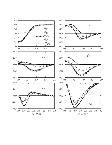
Figure 1: Two-body correlation functions $f_{p}$, as a function of the internucleonic distance. The symbols indicate the correlation functions obtained for symmetric nuclear matter (see text for explanations).

The two-body correlation functions obtained for the $v^{\prime}_{8}$ plus $UIX$ interaction are shown in Fig. 1 for each channel. In the figure, we also show with the diamonds the nuclear matter correlations. These last correlations are obtained with the Euler procedure by using the same healing distances used for finite nuclei but with constant density value of the nuclear matter the saturation point. Analogous results have been obtained for the $v_{14}$ plus $UVII$ interaction.

We would like to point out two features of these results. The first one, is that the various correlations are rather similar for all the nuclei considered. Only the ¹²C results are out of this general trend. This fact indicates that the correlation functions are more sensitive to the characteristics of the nucleon-nucleon interaction than to the shell effects. The second point we want to mention is the difference between the healing distances of the central and tensor channels. In the two-body interaction, the tensor channels are active at larger distances with respect to the central channels, and this produces the consequences on the correlation functions we have just pointed out. It is interesting to notice that the healing for the tensor channels appears at distances larger than the experimental charge radius of the deuteron.

In this discussion the ¹²C nucleus remains an anomaly. The $f_{1}$ correlation is rather similar to those of the other nuclei, all the other two-body correlations are remarkably different, especially $f_{3}$ and $f_{4}$ related to the spin and spin-orbit dependent terms.

Also the nuclear matter results are not on the band formed by the correlations found for the ¹⁶O - ²⁰⁸Pb nuclei. The differences are not so large as those of the ¹²C , but still rather evident. It is remarkable the similarity in the $f_{1}$ channel and in the $f_{5}$ channel, while all the other channels show noticeable differences.

Our calculations are organized in such a way that we first solve the FHNC equation for the scalar correlation only, and in a second step we solve the FHNC/SOC equations with the other state dependent correlation terms. The validity of our solution techniques, from both the theoretical and numerical points of view, can be appreciated by observing the convergence in the density sum rules shown in Tab. 2. In this table we give the normalization of the one- and two-body densities (9) and (10). The $S_{1}$ and $S_{2}$ sum rules have been defined in such a way that all of them are normalized to unity. The results of the table show that the Jastrow-FHNC calculations, those with $f_{1}$ only, produce densities deviating by few parts on a thousand from the correct normalization. The inclusion of state dependent terms in the correlations, the FHNC/SOC calculations, is responsible for an increase of these deviations up to a maximum value of 5.5 %. In many-body systems saturated in spin and isospin one can also test spin and isospin density sum rules. In the systems we are investigating these sum rules are not any more valid.

The main result of our paper is summarized in Tab. 3 where we give the values of the binding energies per nucleon for all the five nuclei considered, and we compare them with the experimental binding energies Audi and Wapstra (1993). In the table we present the various terms contributing to the total energy: the kinetic energy $T$, the two-body interaction, where the the contribution of the first six channels $V^{6}_{2-body}$ and that of the spin-orbit interaction $V_{LS}$ are separately given, the Coulomb interaction $V_{Coul}$ and the three-body force $V_{3-body}$. In the kinetic energy term the contribution of the center of mass motion, calculated as discussed in Co’ et al. (1992), has already been subtracted.

The various terms show some saturation properties. For example the values of kinetic energies per nucleon $T$ increase up to ⁴⁰Ca and then they remain almost stable around a value of about 40 MeV. An analogous behaviour is shown by the $V^{6}_{2-body}$ terms. The contribution per nucleon increases with increasing number of nucleons up to ⁴⁰Ca . After that it is evident that saturation appears in heavier systems.

We have already mentioned the fact that the spin-orbit terms are not treated consistently in the FHNC/SOC computational scheme, but they are evaluated by using some approximation. In any case, in all the nuclei considered, their contributions are of the order of few percent with respect to the $V^{6}_{2-body}$ contributions. As a further test, we have done calculations in ¹⁶O and ⁴⁰Ca switching off the spin-orbit terms in the mean field potential. In this case the spin-orbit partner single particle wave functions are identical. The differences in the total spin-orbit contributions, with respect to the values given in Tab. 3 are within the numerical uncertainty.

The contribution of the Coulomb term $V_{Coul}$ is evaluated within the complete FHNC/SOC computational scheme. As expected, the behaviour with increasing size of the nucleus does not show saturation because of the long range nature of the interaction. The Coulomb terms behave as expected, their contributions increase with increasing number of protons. The apparent inversion of this trend from ⁴⁰Ca to ⁴⁸Ca is due to the representation in terms of energy per nucleon, which in this case is misleading, since the proton number is the same for the two nuclei. In this case it is better to compare the total values of the Coulomb energies, 78.40 MeV for ⁴⁰Ca and 75.36 for ⁴⁸Ca . The 3.8% difference between these to values is due to the different structure of the two nuclei. The inclusion of the Coulomb repulsion reduces the nuclear binding energies. To simplify the reading of the table we give in the raw labeled $T+V(2)$ the intermediate energy value obtained with the two-body force only, Coulomb interaction included. The total binding energies without the three-body forces are all above the experimental values.

In addition to that, there is the contribution of the three-body force. As discussed in Fabrocini et al. (2000), the two terms composing this interactions provide contributions of different sign, the Fujita-Miyazawa term is attractive, while the other term is repulsive. In our calculations the total contribution of the three-body forces is always globally repulsive.

The comparison with the experimental energies indicates a general underbinding of about 3-4 MeV per nucleon. In the general behaviours we have discussed so far, the anomaly of the ¹²C nucleus emerges. In all our calculations the attractive contribution of the $V^{6}_{2-body}$ is relatively smaller than for the other nuclei. As a consequence, this nucleus results barely bound in our calculations. Some crucial physics ingredient relevant in ¹²C while negligible for the other other nuclei is missing in our approach. Probably this has to do with soft deformations of the ¹²C nucleus which we are unable to treat.

The comparison between the two interactions indicates that the $v_{14}$ plus $UVII$ is more attractive than the $v^{\prime}_{8}$ plus $UIX$. This fact is already present when the two-body interaction only is considered. The situation is enhanced by the three-body force, more repulsive for the $UIX$ case than for the $UVII$ one. The contributions of the spin-orbit term in the two cases have different sign, they are attractive for $v^{\prime}_{8}$ and slightly repulsive for $v_{14}$. The differences in the total energies calculated with the two sets of interactions go from a minimum of 5% (¹⁶O ) to a maximum of 18% (²⁰⁸Pb ).

Despite the remarkable differences in the energy, the two interactions produce very similar results in the observables related to the density distributions. For this reason, henceforth, we shall present results obtained with the $v^{\prime}_{8}$ plus $UIX$ interaction only.

In Figs. 2 and 3 we show the one-body density distributions for protons and neutrons respectively. The full lines show the uncorrelated distributions, the dotted lines those obtained by using scalar correlations only $f_{1}$, we call Jastrow these calculations, and the dashed lines the results of the complete calculation. The Jastrow results produce distributions which are smaller at the center of the nucleus with respect to the mean-field distributions. This effect is strongly reduced when all the correlations are included in the calculation. These findings are in agreement with the results of ref. de Saavedra and Renis (1997) where a first-order cluster expansion has been used. It is evident the scarce relevance of short-range correlations in reducing the occupation probability of the 3s1/2 proton state in ²⁰⁸Pb . As pointed out in Anguiano and Co’ (2001), the effect of long-range correlations seems to be main reduction mechanism.

In order to investigate the relative effects of the various correlations on the protons and neutrons distributions we studied the ratio:

$$\Delta_{1}(r)=\frac{\rho(r)-\rho^{o}(r)}{\rho^{o}(r)}$$ (26)

where, as it has been defined in eq. (11), $\rho^{o}(r)$ is the uncorrelated, mean-field, density. The $\Delta_{1}$ ratios are shown in Fig. 4 for all the nuclei under investigation. The behaviour of the various lines indicates more similarity between results obtained with the same type of correlation than between protons and neutrons. This result is quite remarkable because of the large difference between proton and neutron distributions, especially for ⁴⁸Ca and ²⁰⁸Pb .

A direct comparison with the empirical charge density distributions is not very meaningful since the mean-field potential has already been fixed to reproduce, at its best, these distributions. The only statements we can make is whether the inclusion of the correlations improves or not the agreement with the data. For this reason we show in Fig. 5 the ratios

$$\Delta_{2}(r)=\frac{\rho(r)-\rho_{exp}(r)}{\rho_{exp}(0)}$$ (27)

where the experimental charge distributions have been taken from Jager and Vries (1987). The inclusion of correlations lowers the charge density distributions at the center of the nuclei. If scalar correlation only are considered the effect is too large. When all the correlations are included the effect is strongly reduced and the agreement with the empirical densities improves.

The effects of the short-range correlations are better shown on the two-body density matrices (10). We define the operator dependent two-body density matrices as:

$$\rho^{\alpha\beta,p}_{2}({\bf r}_{1},{\bf r}_{2})=\frac{A(A-1)}{<\Psi|\Psi>}$$ (28)

$$\int dx_{3}...dx_{A}\,\Psi^{*}(x_{1},x_{2},x_{3},...,x_{A}){\cal P}^{\alpha}(1)O^{p}(x_{1},x_{2}){\cal P}^{\beta}(2)\Psi(x_{1},x_{2},x_{3},...,x_{A})$$

where we have indicated with ${\cal P}^{\alpha}(i)$ the operator selecting protons or neutrons and we have understood the trace on the spins and isospins of the particles 1 and 2. We calculate the values of (28) in terms of relative distance $r_{12}=|{\bf r}_{1}-{\bf r}_{2}|$ between the two considered nucleons

$$\rho^{\alpha\beta,p}_{2}(r_{12})=\int d{\bf R}_{12}\rho^{\alpha\beta,p}_{2}({\bf r}_{1},{\bf r}_{2})$$ (29)

where ${\bf R_{12}}=({\bf r}_{1}+{\bf r}_{2})/2$ is the center of mass coordinate of the pair. In the FHNC/SOC computational scheme, we calculated the two-body density matrices as:

$$\rho^{\alpha\beta,2k_{3}-1+l_{3}}_{2}({\bf r}_{1},{\bf r}_{2})=\frac{f_{2k_{1}-1+l_{1}}(r_{12})f_{2k_{2}-1+l_{2}}(r_{12})}{f_{1}^{2}(r_{12})}\Bigg{\{}I^{k_{1}k_{3}k_{2}}A^{k_{2}}\chi^{\alpha\beta}_{l_{1}+l_{2}+l_{3}}\rho^{\alpha\beta}_{2,dir}({\bf r}_{1},{\bf r}_{2})$$

$$+\Big{(}I^{k_{4}k_{1}k_{5}}I^{k_{2}k_{3}k_{5}}A^{k_{5}}\rho_{2,exc}^{\alpha\beta}({\bf r}_{1},{\bf r}_{2})+I^{k_{4}k_{1}k_{5}}I^{k_{2}k_{3}k_{6}}I^{k_{5}k_{6}2}\rho_{2,excj}^{\alpha\beta}({\bf r}_{1},{\bf r}_{2})\Big{)}\Delta^{k_{4}}\sum_{l_{4}=0}^{1}\chi^{\alpha\beta}_{l_{1}+l_{2}+l_{3}+l_{4}}\Bigg{\}}$$

where a sum on the repeated indexes is understood and the symbols of eq. (23) have been used.

Let’s consider first the Jastrow case, where only $f_{1}$ correlation functions are present, i.e. $2k_{1}-1+l_{1}=2k_{2}-1+l_{2}=1$. In this case, apart from a normalization factor, eq. (28) gives the probability density of finding two nucleons with isospin third-components $\alpha$ and $\beta$ at the distance $r_{12}$. These scalar two-body density functions, or probability densities, are shown in Figs. 6, 7 and 8, for all the nuclei we have investigated. The dotted lines represent the uncorrelated joint probability densities of finding the two nucleons as often given in the literature, see for example Benhar et al. (1993). This joint probabilities are obtained as product of the uncorrelated one-body densities. This definition of the uncorrelated two-body density can be meaningful from the probabilistic point of view, but it is misleading in our framework, since it corresponds to use only the first, direct, term of eq. (12). In fermionic systems, the uncorrelated two-body density is given by the full expression (12) containing also the exchange term. These complete uncorrelated two-body densities, are shown in Figs. 6, 7 and 8 by the full lines. The effects of the short-range correlations can be deduced by comparing these lines with the dashed-dotted lines obtained with the $f_{1}$ scalar correlations only, we call these Jastrow results, and with the dashed lines showing the full FHNC/SOC results.

In all our results, the correlations reduce the values of the two-body densities at short internucleon distances. The exchange term of the uncorrelated density, already contributes to this reduction, but the major effect is produced by the short-range correlations, and mainly by the scalar correlations. The effects of nucleon-like two-body densities are rather similar, as it can be seen comparing Figs. 6 and 8. When the pair of nucleons is composed by different particles the situation slightly changes. Beside to the strong reductions at small distances, the correlations produce enhancements around 2 fm in all the nuclei considered.

In order to discuss the effects of the correlations on the other operator dependent two-body densities (28), we show in Figs. 9 and 10 the results for the ²⁰⁸Pb nucleus only. The results of the other nuclei considered have similar features Bisconti (2005). In these figures, we used the same line conventions of Figs. 6, 7 and 8. When the external particles are nucleons of the same type, i.e. $\alpha=\beta$ in eqs. (28) - (III), the isospin trace in eq. 28 is one. In this case, the p=1,2,3 two-body densities are equal, respectively, to those calculated with p=2,4,6. The same idea can be expressed more formally by stating that, in eq. (III) for $\alpha=\beta$ we have $\rho^{\alpha\alpha,2k-1}_{2}(r_{12})=\rho^{\alpha\alpha,2k}_{2}(r_{12})$, since $\chi_{n}^{\alpha\alpha}=1$ for every value of $n$. For this reason, in Fig. 6, we present only the p=3 and p=5 two-body densities for both proton-proton and neutron-neutron cases. In the proton-neutron case the two-body densities are different in every channel.

We first notice that tensor two-body densities, p=5, and also p=6 in Fig. 7, are different from zero only in the full FHNC/SOC calculations. This occours because in order to get a spin trace different from zero in eq. 28 at least two tensor operators are needed. In Fig. 7 also the p=3 spin density is different from zero only in the FHNC/SOC case. The reason is that, in the calculation of this density,for the uncorrelated and the Jastrow cases, the first term of eq. (12), the direct one, is zero because of the spin trace, while the exchange term is zero because of the different isospin third component.

We observe from Figs. 6 and 7 that the effects of the correlations are analogous to those already discussed for the scalar two-body densities: the values of the densities is strongly reduced at short internucleonic distances. In addition to that it is worth to mention the change of sign in the isospin, p=2, densities in the proton-neutron case. The most remarkable feature is the range of the various densities. The scalar densities of Figs. 6, 7 and 8 and the isospin densities, p=2, extend up to relative distances comparable to the dimensions of the nucleus, 15 fm. On the contrary, all the other two-body densities have much smaller ranges, of the order of 3-4 fm. These features are present in all the nuclei considered Bisconti (2005).

IV SUMMARY AND CONCLUSIONS

With this paper we made an important step forward in our project aimed to provide a microscopical description of medium-heavy nuclei, by using the CBF theory. With respect to the works of Refs. Fabrocini et al. (1998, 2000) we have applied for the first time the FHNC/SOC computational scheme to nuclei with different number of protons and neutrons and in the $jj$ coupling scheme. We have used two different sets of microscopic interactions: the Argonne $v^{\prime}_{8}$ implemented with the Urbana IX three-body force, and the truncated Urbana $v_{14}$ plus the Urbana VII three-body force. Binding energies have been presented in Tab. 3 and this is the main result of our work. With the noticeable exception of the ¹²C nucleus, our binding energies are about 3-4 MeV/nucleon above the experimental ones, consistently with our previous results Fabrocini et al. (2000) and with those obtained in nuclear matter.

In our calculations we did not include the contributions of the spin-orbit terms of the correlation and of the p$>$ 8 terms of the two-body potential, which in Fabrocini et al. (2000) have been estimated by means of a local density interpolation of the nuclear matter results. These contributions are attractive and of the order of 1 MeV/nucleon. This produces differences with the experimental values of the order of those presented in Fabrocini et al. (2000) where only the ¹⁶O and ⁴⁰Ca nuclei were considered. A number of possible sources of the remaining disagreement should be investigated such as the three-body correlations and perturbative corrections of the two-body correlations.

The ¹²C nucleus, strongly underbound, stands out of this general trend. As we have already said some specific characteristics of this nucleus, not relevant in the other nuclei we have considered, is not properly treated in our calculations. We think this could be the presence of deformation phenomena.

Short-range correlations produce small effects on the one-body density distributions. The distributions at the center of the nucleus are lowered by the correlations. This effect is relatively large when only scalar correlations are used, and it is strongly reduced when the other terms of the correlations are included. These results are in agreement with the findings of de Saavedra and Renis (1997) where a simple first-order expansion of the density has been used.

The study of the two-body densities show that the short-range correlations strongly reduce the probability of finding two nucleons at distances smaller than 0.5-0.6 fm. The scalar and isospin, two-body densities, extend on the full nuclear volume, while the other densities have a maximum range of about 3 fm.

Our work shows that microscopic variational calculations for medium-heavy nuclei have reached the same degree of accuracy as nuclear matter calculations. Our approach provides a good description of the short-range correlations, but it shows some deficiency related to the proper inclusion of long-range correlations. The next obvious step would be to extend the theory to have a better treatment of these last type of correlations.

		12C	16O	40Ca	48Ca	208Pb
$v^{\prime}_{8}$ +	$d_{c}$	1.20	2.10	2.15	2.10	2.20
$UIX$	$d_{t}$	3.30	3.70	3.66	3.70	3.60
$v_{14}$ +	$d_{c}$	1.40	2.10	2.15	2.10	2.20
$UVII$	$d_{t}$	3.30	3.80	3.86	3.90	3.80

Table 1: Values, in fm, of the healing distances, obtained minimizing the energy functional (2) with the interactions we have used in our calculations.

		12C	16O	40Ca	48Ca	208Pb
$S^{p}_{1}$	$(J)$	1.000	1.000	1.000	1.000	0.999
$S^{p}_{1}$	$(SOC)$	0.997	1.006	1.008	1.013	1.024
$S^{n}_{1}$	$(J)$	1.000	1.000	1.000	0.999	0.999
$S^{n}_{1}$	$(SOC)$	0.997	1.006	1.008	1.021	1.027
$S_{2}$	$(J)$	1.004	1.003	1.001	1.000	0.998
$S_{2}$	$(SOC)$	0.996	1.025	1.022	1.042	1.055

Table 2: Normalization of the one- and two-body densities $S_{1}$ and $S_{2}$ respectively. For the one-body densities we give separately the contributions of the protons ($p$) and neutrons ($n$). The label $J$ (Jastrow) indicates the calculation done with the scalar, $f_{1}$, correlation only, while the $SOC$ labels indicate the results of the complete calculation.

		12C	16O	40Ca	48Ca	208Pb
	$T$	27.13	32.33	41.06	39.64	39.56
	$V^{6}_{2-body}$	-29.13	-38.15	-48.97	-46.60	-48.43
	$V_{LS}$	-0.25	-0.38	-0.39	-0.35	-0.45
$v^{\prime}_{8}$ +	$V_{Coul}$	0.67	0.86	1.96	1.57	3.97
$UIX$	$T+V(2)$	-1.58	-5.34	-6.34	-5.74	-5.35
	$V_{3-body}$	0.66	0.86	1.76	1.61	1.91
	$E$	-0.91	-4.49	-4.58	-4.14	-3.43
	$T$	24.63	29.25	37.70	36.47	36.48
	$V^{6}_{2-body}$	-27.08	-35.84	-47.16	-44.86	-46.87
	$V_{LS}$	0.05	0.03	0.07	0.09	0.04
$v_{14}$ +	$V_{Coul}$	0.68	0.88	2.02	1.59	4.03
$UVII$	$T+V(2)$	-1.72	-5.68	-7.37	-6.71	-6.32
	$V_{3-body}$	0.54	0.69	1.28	1.15	1.41
	$E(UIX)$	-1.18	-4.99	-6.09	-5.56	-4.91
	$E_{exp}$	-7.68	-7.97	-8.55	-8.66	-7.86

Table 3: Energies per nucleon in MeV. We have indicated with $T$ the kinetic energy, with $V^{6}_{2-body}$ the contribution of the first six channels of the two-body interaction, with $V_{LS}$ the spin-orbit contribution, with $V_{Coul}$ the contribution of the Coulomb interaction and with $V_{3-body}$ the total contribution of the three-body force. The raws labeled $T+V(2)$ show the energies obtained by considering the two-body interactions only. The experimental values are taken form Audi and Wapstra (1993).

Figure 2: Proton density distributions. The full lines are the mean field distributions, the dotted ones have been obtained by using scalar correlations ($f_{1}$) only, and the dashed lines show the results of the complete calculation.

Figure 3: The same as Fig. 2, for the neutron density distributions.

Figure 4: Normalized ratios (26) for proton and neutron distributions. The meaning of the lines is given in the legend, where we have indicated with $J$ the results obtained with scalar correlation ($f_{1}$) only, and with $SOC$ the results of the full calculation.

Figure 5: Normalized ratios (27) for charge density distributions. The meaning of the lines is given in the legend.

Figure 6: Proton-proton scalar (p=1) two-body distributions (29) as a function of the internucleonic distance. The dotted lines show the uncorrelated two-body distributions calculated by considering only the first term of eq. (12), the direct one. The full lines show the total uncorrelated two-body distributions as given by eq. (12). The other two types of lines indicate the results obtained with scalar correlations only (Jastrow) and in the complete calculation (SOC).

Figure 7: The same as Fig. 6 for the proton-neutron case. The dotted and full lines coincide, since the exchange term of eq. (12) is zero.

Figure 8: The same as Fig. 6 for the neutron-neutron.

Figure 9: Proton-proton and neutron-neutron two-body distribution functions (29) of ²⁰⁸Pb nucleus. As discussed in the text, for equal particles, the p=2,4,6 distribution functions are respectively equal to the p=1,3,5 ones.

Figure 10: The same as Fig. 9 for the proton-neutron case.

References

- Pudliner et al. (1995) B. S. Pudliner, V. Pandharipande, J. Carlson, and R. B. Wiringa, Phys. Rev. Lett. 74, 4396 (1995).
- Pudliner et al. (1997) B. S. Pudliner, V. Pandharipande, J. Carlson, S. Pieper, and R. B. Wiringa, Phys. Rev. C 56, 1720 (1997).
- Pieper (2005) S. Pieper, Nucl. Phys. A 751, 516 (2005).
- Schmid et al. (1991) K. W. Schmid, H. Müther, and R. Machleidt, Nucl. Phys. A 530, 14 (1991).
- Dickhoff and Barbieri (2004) W. H. Dickhoff and C. Barbieri, Prog. Part. Nucl. Phys. 52, 377 (2004).
- Navrátil et al. (2000) P. Navrátil, J. P. Vary, and B. R. Barrett, Phys. Rev. C 62, 054311 (2000).
- Forssén et al. (2005) C. Forssén, P. Navrátil, W. E. Ormand, and E. Caurier, Phys. Rev. C 71, 044312 (2005).
- Heisenberg and Mihaila (1999) J. H. Heisenberg and B. Mihaila, Phys. Rev. C 59, 1440 (1999).
- Mihaila and Heisenberg (1999) B. Mihaila and J. H. Heisenberg, Phys. Rev. C 60, 054303 (1999).
- Dean and al. (2005) D. J. Dean and al., Nucl. Phys. A 752, 299c (2005).
- Neff and Feldmeier (2003) T. Neff and H. Feldmeier, Nucl. Phys. A 713, 311 (2003).
- Roth et al. (2004) R. Roth, T. Neff, H. Hergert, and H. Feldmeier, Nucl. Phys. A 745, 3 (2004).
- Rosati (1982) S. Rosati, A. Molinari ed., From Nuclei to particles: Proc. Int. School E. Fermi, course LXXIX (North-Holland, 1982).
- Co’ et al. (1992) G. Co’, A. Fabrocini, S. Fantoni, and I. E. Lagaris, Nucl. Phys. A 549, 439 (1992).
- Co’ et al. (1994) G. Co’, A. Fabrocini, and S. Fantoni, Nucl. Phys. A 568, 73 (1994).
- de Saavedra et al. (1996) F. Arias de Saavedra, G. Co’, A. Fabrocini, and S. Fantoni, Nucl. Phys. A 605, 359 (1996).
- Fabrocini et al. (1998) A. Fabrocini, F. Arias de Saavedra, G. Co’, and P. Folgarait, Phys. Rev. C 57, 1668 (1998).
- Fabrocini et al. (2000) A. Fabrocini, F. Arias de Saavedra, and G. Co’, Phys. Rev. C 61, 044302 (2000).
- Wiringa et al. (1995) R. B. Wiringa, V. G. J. Stoks, and R. Schiavilla, Phys. Rev. C 51, 38 (1995).
- Lagaris and Pandharipande (1981a) I. Lagaris and V. R. Pandharipande, Nucl. Phys. A 359, 331 (1981a).
- Lagaris and Pandharipande (1981b) I. Lagaris and V. R. Pandharipande, Nucl. Phys. A 359, 349 (1981b).
- Schiavilla et al. (1986) R. Schiavilla, V. R. Pandharipande, and R. B. Wiringa, Nucl. Phys. A 449, 219 (1986).
- Bisconti (2005) C. Bisconti, Ph.D. thesis, Università di Lecce (2005), unpublished.
- Fujita and Miyazawa (1957) J. Fujita and H. Miyazawa, Prog. Theor. Phys. 17, 360 (1957).
- Pandharipande and Wiringa (1979) V. Pandharipande and R. B. Wiringa, Rev. Mod. Phys. 51, 821 (1979).
- Fantoni and Rosati (1979) S. Fantoni and S. Rosati, Phys. Lett. B 84, 23 (1979).
- Carlson et al. (1983) J. Carlson, V. R. Pandharipande, and R. B. Wiringa, Nucl. Phys. A 401, 59 (1983).
- Audi and Wapstra (1993) G. Audi and A. H. Wapstra, Nucl. Phys. A 565, 1 (1993).
- de Saavedra and Renis (1997) F. Arias de Saavedra, G. Co’ and M. M. Renis, Phys. Rev. C 55, 673 (1997).
- Anguiano and Co’ (2001) M. Anguiano and G. Co’, Jour. Phys. G 27, 2109 (2001).
- Jager and Vries (1987) C. W. D. Jager and C. D. Vries, At. Data Nucl. Data Tables 36, 495 (1987).
- Benhar et al. (1993) O. Benhar, V. R. Pandharipande, and S. C. Pieper, Rev. Mod. Phys. 65, 817 (1993).