Neutron star cooling constraints for color superconductivity in hybrid stars

Abstract

We apply the recently developed $\mathrm{Log\,N}$-$\mathrm{Log\,S}$ test of compact star cooling theories for the first time to hybrid stars with a color superconducting quark matter core. While there is not yet a microscopically founded superconducting quark matter phase which would fulfill constraints from cooling phenomenology, we explore the hypothetical 2SC+X phase and show that the magnitude and density-dependence of the X-gap can be chosen to satisfy a set of tests: temperature - age ($\mathrm{T}$-$\mathrm{t}$), the brightness constraint, $\mathrm{Log\,N}$-$\mathrm{Log\,S}$, and the mass spectrum constraint. The latter test appears as a new conjecture from the present investigation.

I Introduction

Recently, preparations for terrestrial laboratory experiments with heavy-ion collisons have been started, where it is planned to access the high-density/ low temperature region of the QCD phase diagram and explore physics at the phase boundary between hadronic and quark matter, e.g., within the CBM experiment at FAIR Darmstadt.

Predictions for critical parameters in this domain of the temperature-density plane are uncertain since they cannot be checked against Lattice-QCD simulations which became rather precise at zero baryon densities. Chiral quark models have been developed and calibrated with these results. They can be extended into the finite-density domain and suggest a rich structure of color superconducting phases. These hypothetical phase structures shall imply consequences for the structure and evolution of compact stars, where the constraints from mass and radius measurements as well as from the cooling phenomenology have recently reached an unprecedented level of precision which allows to develop decisive tests of models for high-density QCD matter.

Among compact stars (we will address them also with the general term neutron stars (NSs)) one can distiguish three main classes according to their composition: hadron stars, quark stars (bare surfaces or with thin crusts), and hybrid stars (HyS). The latter are the subject of the present study.

Observations of the surface thermal emission of NSs is one of the most promising ways to derive detailed information about processes in interiors of compact objects (see Page:2005fq ; Page:2004fy ; Yakovlev:1999sk for recent reviews). In Popov:2004ey (Paper I hereafter) we proposed to use a population synthesis of close-by cooling NSs as an addtional test for theoretical cooling curves. This tool, based on calculation of the $\mathrm{Log\,N}$-$\mathrm{Log\,S}$ distribution, was shown to be an effective supplement to the standard $\mathrm{T}$ - $\mathrm{t}$ (Temperature vs. age) test. In Paper I we used cooling curves for hadron stars calculated in Blaschke:2004vq . Here we study cooling curves of HyS calculated in Grigorian:2004jq (Paper II hereafter).

Except $\mathrm{T}$ - $\mathrm{t}$ and $\mathrm{Log\,N}$-$\mathrm{Log\,S}$ we use also the brightness constraint test (BC) suggested in Grigorian:2005fd . We apply altogether three tests – $\mathrm{T}$-$\mathrm{t}$, $\mathrm{Log\,N}$-$\mathrm{Log\,S}$, and BC – to five sets of cooling curves of HyS. In the next section we describe calculation of these curves. In Section III we discuss the population synthesis scenario. After that we present our results which imply the conjecture of a new mass spectrum constraint from Vela-like objects. In Section 5 we discuss the results and present our conclusions in Section  6.

II Cooling curves for hybrid stars

II.1 Hybrid stars

The description of compact star cooling with color superconducting quark matter interior is based on the approach introduced in Paper II which will be briefly reviewed here, see also Blaschke:2005dc for a recent summary. A nonlocal, chiral quark model is employed which supports compact star configurations with a rather large quark core due to the relatively low critical densities for the deconfinement phase transition from hadronic matter to color superconducting quark matter. In the interior of the compact star in late cooling stages, when the temperature is well below the opacity temperature $T_{\rm opac}\sim 1$ MeV for neutrino untrapping, four phases of quark matter are possible: normal quark matter (NQ), two-flavor superconducting matter (2SC), a mixed phase of both (NQ-2SC) and the color-flavor-locking phase (CFL). The state-of-the-art calculations for a three-flavor quark matter phase diagram within a chiral (NJL) quark model of quark matter and selfconsistently determined quark masses are described in Refs. Ruster:2005jc ; Blaschke:2005uj ; Abuki:2004zk .

The detailed structure of the phase diagram in these models still depends on the strength parameter $G_{D}$ of the diquark coupling (and on the formfactor of the momentum space regularization, see Aguilera:2004ag ). For all values of $G_{D}$ no stable hybrid stars with a CFL phase have been found yet, see Buballa:2003qv , and Refs. therein. We will restrict us here to the discussion of 2SC and NQ phases.

The 2SC phase occurs at lower baryon densities than the CFL phase Steiner:2002gx ; Neumann:2002jm . For applications to compact stars the omission of the strange quark flavor is justified by the fact that chemical potentials in central parts of the stars barely reach the threshold value at which the mass gap for strange quarks breaks down and they may appear in the system Gocke:2001ri .

It has been shown in Blaschke:2003yn that a nonlocal chiral quark model with the Gaussian formfactor ansatz leads to an early onset of the deconfinement transition so that hybrid stars with large quark matter cores Grigorian:2003vi can be discussed.

In describing the hadronic part of the hybrid star, as in Blaschke:2004vq , we adopt the Argonne $V18+\delta v+UIX^{*}$ model for the EoS Akmal:1998cf , which is based on recent data for the nucleon-nucleon interaction with the inclusion of a parameterized three-body force and relativistic boost corrections.

Actually we continue to adopt an analytic parameterization of this model by Heiselberg and Hjorth-Jensen Heiselberg:1999fe , where the fit is done for $n<4~{}n_{0}$ with $n_{0}=0.16$ fm^-3 being the nuclear saturation density. This EoS fits the symmetry energy to the original Argonne $V18+\delta v+UIX^{*}$ model in the mentioned density interval and smoothly incorporates causality constraints at high densities. The threshold density for the DU process is $n_{c}^{\rm DU}\simeq~{}5.19~{}n_{0}$, i.e. it occurs in stars with masses exceeding $M_{c}^{\rm DU}\simeq 1.839~{}M_{\odot}$).

II.2 Cooling

For the calculation of the cooling of the hadronic part of the hybrid star we use the same model as in Blaschke:2004vq . The main processes are the medium modified Urca (MMU) and the pair breaking and formation (PBF) processes for our adopted EoS of hadronic matter. For a recent, more detailed discussion of these processes and the role of the $3P_{2}$ gap, see Grigorian:2005fn .

The possibilities of pion condensation and of other so called exotic processes are suppressed since in the model Blaschke:2004vq these processes may occur only for neutron star masses exceeding $M_{c}^{\rm quark}=1.214~{}M_{\odot}$. The DU process is irrelevant in this model up to very large neutron star masses $M>1.839~{}M_{\odot}$. The $1S_{0}$ neutron and proton gaps are taken the same as those shown by thick lines in Fig. 5 of Ref. Blaschke:2004vq . We pay particular attention to the fact that the $3P_{2}$ neutron gap is additionally suppressed by the factor $0.1$ compared to that shown in Fig. 5 of Blaschke:2004vq . This suppression is motivated by the result of the recent work in Schwenk:2003bc and is required to fit the cooling data.

For the calculation of the cooling of the quark core in the hybrid star we use the model introduced in Blaschke:2004vq . We incorporate the most efficient processes: the quark direct Urca (QDU) processes on unpaired quarks, the quark modified Urca (QMU), the quark bremsstrahlung (QB), the electron bremsstrahlung (EB), and the massive gluon-photon decay (see Blaschke:1999qx ). Following Jaikumar:2001hq we include the emissivity of the quark pair formation and breaking (QPFB) processes. The specific heat incorporates the quark contribution, the electron contribution and the massles and massive gluon-photon contributions. The heat conductivity contains quark, electron and gluon terms.

The 2SC phase has one unpaired color of quarks (say blue) for which the very effective quark DU process works and leads to a too fast cooling of the hybrid star in disagreement with the data Grigorian:2004jq . We have suggested to assume a weak pairing channel which could lead to a small residual pairing of the hitherto unpaired blue quarks. We call the resulting gap $\Delta_{X}$ and show that for a density dependent ansatz

$$\Delta_{\mathrm{X}}=\Delta_{0}\,\exp{\left[-\alpha\,\left(\frac{\mu-\mu_{c}}{\mu_{c}}\right)\right]}$$ (1)

with $\mu$ being the quark chemical potential, $\mu_{c}=330$ MeV. Here we use different values of $\alpha$ and $\Delta_{0}$, which are given in Table 1 characterizing the model.

The physical origin of the X-gap remains to be identified. It could occur, e.g., due to quantum fluctuations of color neutral quark sextett complexes Barrois:1977xd . Such calculations have not yet been performed with the relativistic chiral quark models.

For sufficiently small $G_{D}$, the 2SC pairing may be inhibited at all. In this case, due to the absence of this competing spin-0 phase with large gaps, one may invoke a spin-1 pairing channel in order to avoid the DU problem. In particular the color-spin-locking (CSL) phase Schafer:2000tw may be in accordance with cooling phenomenology as all quark species are paired and the smallest gap channel may have a behavior similar to Eq. (1), see Aguilera:2005tg . A consistent cooling calculation for this phase, however, requires the evaluation of neutrino emissivities (see, e.g. Schmitt:2005wg and references therein) and transport coefficients, which is still to be performed.

Gapless superconducting phases can occur when the diquark coupling parameter is small so that the pairing gap is of the order of the asymmetry in the chemical potentials of the quark species to be paired. Interesting implications for the cooling of gapless CFL quark matter have been conjectured due to the particular behavior of the specific heat and neutrino emissivities Alford:2004zr . For reasonable values of $G_{D}$, however, these phases do occur only at too high temperatures to be relevant for late cooling, if a stable hybrid configuration with these phases could be achieved at all Blaschke:2005uj .

The weak pairing channels are characterized by gaps typically in the interval $10~{}$ keV $\div 1~{}$MeV, see discussion of different attractive interaction channels in paper Alford:2002rz .

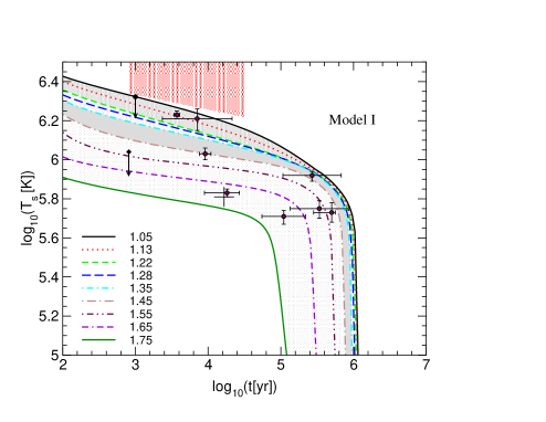
Figure 1: Hybrid star cooling curves for Model I. Different lines correspond to compact star mass values indicated in the legend (in units of $M_{\odot}$), data points with error bars are taken from Ref. Page:2004fy . For the explanation of shaded areas, see text.

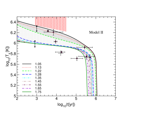
Figure 2: Same as Fig. 1 for Model II.

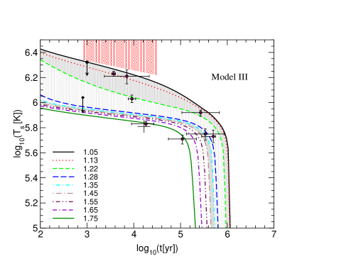
Figure 3: Same as Fig. 1 Model III.

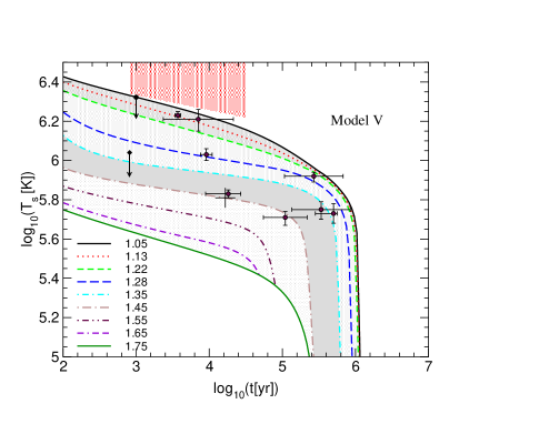
Figure 4: Same as Fig. 1 for Model IV.

In the figures we present $\mathrm{T}$-$\mathrm{t}$ plots for four models used in this paper. On each plot data points for known cooling NSs are added (see details in Grigorian:2005fd ). The hatched trapeze-like region represents the brightness constraint (BC). For each model nine cooling curves are shown for configurations with mass values corresponding to the binning of the population synthesis calculations explained in the next section.

Clearly, all models satisfy the BC. As for the $\mathrm{T}$-$\mathrm{t}$ test the situation is different. The Model II does not pass the test because even the highest mass configuration (which corresponds to the coolest HyS) cannot explain the lowest data points. So, in the Table 1 it is marked that the model does not pass the test.

In this work we want to introduce a more detailed measure for the ability of a cooling model to describe observational data in the temperature-age diagram. We assign five grey values to regions of compact star masses in the $T-t$ diagram which encode the likelihood that stars in that mass interval can be found in the solar neighborhood, according to the population synthesis scenario, see Fig. 5. The darkest grey value, for example, corresponds to the mass interval $1.35\div 1.45$ M_⊙ for which the population sysnthesis predicts the most objects. According to this refined mass spectrum criterion a cooling model is optimal when the darkness of the grey value is in accordance with the number of observed objects in that region of the temperature-age diagram. This criterion is ideally fulfilled for Model IV, where with only one exception all objects are found in the two bands with darker grey values whereas for Models I - III about half of the objects are situated in light grey or even white regions.

III Population synthesis scenario

Population synthesis is a frequently used technique in astrophysics described, e.g., in the review Popov:2004gw where further references can be found. The idea is to construct an evolutionary scenario for an artificial population of certain astronomical objects. The comparison with observations gives the opportunity to test our understanding of evolutionary laws and initial conditions for these sources.

The scenario that we use in this paper is nearly identical to the one used in Paper I. We just briefly recall the main elements and then describe the only small difference in the mass spectrum.

The main ingredients of the population synthesis model we use are: the initial distribution of NSs and their birth rate; the velocity distribution of NSs; the mass spectrum of NSs; cooling curves and interstellar absorption.

In this series of papers in which we use the population synthesis model as a test of the theory of thermal evolution of NSs, we assume that the set of cooling curves is the most undetermined igredient. So, we make an attempt to test it. The cooling curves used in this paper are described in Sec. 2.

We assume that NSs are born in the Galactic disc and in the Gould Belt. The disc region is calculated up to 3 kpc from the Sun, and is assumed to be of zero thickness. The birth rate in the disc part of the distribution is taken as 250 NS per Myr. The Gould Belt is modeled as a flat disc-like structure with a hole in the center (see the Belt description in p97 ). The inclination of the Belt relative to the galactic plane is $18^{\circ}$. The NS birth rate in the Belt is 20 per Myr.

The velocity distribution of NSs is not well known. In our calculations we use the one proposed by Arzoumanian:2001dv . This is a bimodal distribution with two maxima at $\sim 127$ and $\sim 707$ km s^-1. Recent results question this bimodality Hobbs:2005yx . However, since the time scales in our calculations typically are not very long, the exact form of the distribution is not very important.

For the calculation of the column density towards a given NS we use the same approximation as we used before. It depends only on the distance to the galactic center and the height above the galactic plane (see Fig. 1 in Popov:1999qn ). The detailed structure of the interstellar medium (ISM) is not taken into account, except the Local Bubble, which is modeled as a 140-pc sphere centered on the Sun.

The mass spectrum is a crucial ingredient of the scenario. The main ideology of its derivation is the same as given in Popov:2003iq . At first we take all massive stars which can produce a NS (spectral classes B2-08) from the HIPPARCOS catalogue with parallaxies $<0.002$ arcsec. Then for each spectral class we assign a mass interval. In the next step using calculations by woosley we obtain the baryon masses of compact remnants. Then we have to calculate the gravitational mass. In this paper, unlike our previous studies where we just used the formula from Timmes:1995kp $M_{\mathrm{bar}}-M_{\mathrm{grav}}=\alpha\,M_{\mathrm{grav}}^{2}$ with $\alpha=0.075$, we use $M_{\mathrm{grav}}$ accurately calculated for the chosen configuration. Since the approximation from Timmes:1995kp is very good the difference with the mass spectrum we used in Paper I is tiny, and appears only in three most massive bins of our spectrum.

In this paper we slightly rebinned the mass spectrum in order to have a better coverage of the cooling behaviour for the chosen configurations. As before we use eight mass bins defined by their borders: 1.05; 1.13; 1.22; 1.28; 1.35; 1.45; 1.55; 1.65; 1.75 $M_{\odot}$, see Fig. 5. The critical mass for the formation of a quark core is close to 1.22 $M_{\odot}$. Therefore, bins are chosen such that the first two represent purely hadronic stars. Bins are of different width. Outermost bins have a width 0.1 $M_{\odot}$. We do not expect HyS with masses M $<1.05$ M_⊙. The upper boundary of the eighth bin lies close to the maximum mass allowed by the chosen configuration.

Following the suggestion by Timmes:1995kp we make runs for two modifications of the mass spectrum. Except the usage of the full range of masses we produce, in addition, calculations for the truncated spectrum. In this case contributions of the first two bins are added to the third bin. This situation reflects the possibility that stars with $M\stackrel{{\scriptstyle<}}{{\sim}}11\,M_{\odot}$ can produce NSs of similar masses close to ${\sim}1.27\,M_{\odot}$.

As in Paper I we neglect effects of a NS atmosphere, and use pure blackbody spectra. As we do not address particular sources this seems to be a valid approximation.

Figure 5: The adopted mass spectrum, binned over eight intervals of different widths. The non-truncated spectrum is shown (see text).

The population synthesis code calculates spatial trajectories of NSs with the time step $10^{4}$ yrs. For each point from the set of cooling curves we have the surface temperature of the NS. Calculations for an individual track are stopped at the age when the hottest NSs (for all five models here this is a star with $M=1.1\,M_{\odot}$, unless the truncated mass spectrum is used) reaches the temperature $10^{5}$ K. Such a low temperature is beyond the registration limit for ROSAT even for a very short distance from the observer. With the known distance from the Sun and the ISM distribution we calculate the column density. Finally, count rates are calculated using the ROSAT response matrix. Results are summarized along each individual trajectory. We calculate 5,000 tracks for each model. Each track is applied to all eight cooling curves. With a typical cooling timescale of about 1 Myr, we obtain $\sim 4\cdot 10^{6}$ “sources”. The results are then normalized to the chosen NS formation rate (290 NSs in the whole region of the problem).

IV Numerical results

In this section we present results of our calculations for four models, characterized by different sets of the two-parameter ansatz for the X-gap, Eq. (1), see Table 1. $\mathrm{Log\,N}$-$\mathrm{Log\,S}$ curves are given for two values of the Gould Belt radius ($R_{\mathrm{belt}}=300$ and 500 pc), and for two variants of the mass spectrum (full and truncated).

The modeled $\mathrm{Log\,N}$-$\mathrm{Log\,S}$ curves are confronted with data for close-by, young cooling NSs observed by ROSAT. This data set includes the Magnificent Seven (seven dim radio-quiet NSs), radio pulsars, Geminga and a geminga-like source (see the list and details in Popov:2003hq ). The error bars correspond to poissonian errors (i.e. square root of the number of sources). An important upper limit is added Rutledge:2003kg which represents an estimate of unidentified cooling NSs in the ROSAT Bright Source Catalogue (BSC).

Model I is the best model from Paper II. An important feature of this model is that cooling curves cover data points in the $\mathrm{T}$-$\mathrm{t}$ plot very uniformly.

The parameters of the Model II were specifically chosen in such a way, that it is possible to demonstrate the fact that the $\mathrm{Log\,N}$-$\mathrm{Log\,S}$ test can be successful for a set that fails to pass the $\mathrm{T}$-$\mathrm{t}$ test. Even for the highest possible mass it is imposible to explain cold stars, but as the $\mathrm{Log\,N}$-$\mathrm{Log\,S}$ test is not sensitive to what is happening with massive NSs it does not influence the results of the population synthesis.

Model III is an attempt of a compromise to fulfill at least marginally all three tests. It has s smaller gap than the Model I, and unlike Model II it has a non-zero value of $\alpha$. It can explain all data points in the $\mathrm{T}$-$\mathrm{t}$ plot within an available mass range resorting, however, to the very unlikely objects with masses above 1.5 M_⊙.

Models IV assumes a steeper density dependence of the X-gap than all previous ones. It is thus possible to spread the set of cooling curves over the existing cooling data already for mass variations within the range of most probable mass values $1.25\pm 0.25$ M_⊙ in Fig. 5. Using these models it is possible to describe even the Vela pulsar being a young, nearby and rather cool object, within this mass range.

V Discussion

In the present paper we were to find a set of parameters for which all three tests ($\mathrm{T}$-$\mathrm{t}$, $\mathrm{Log\,N}$-$\mathrm{Log\,S}$, and BC) can be successfully passed? Are these tests sufficient to constrain a model or is it necessary to assume additional constraints?

For the $\mathrm{T}$-$\mathrm{t}$ test it is necessary to cover the observed points by curves from a relatively wide range of masses which are consistent with known data on inital NS mass distribution (for example, data on masses of not-accreted, i.e. mainly secondary, companions of double NS systems). For the Model III (see Fig. 3), for example, this is not the case as a number of data points seems to correspond to a narrow mass range slightly below the critical mass $1.22\,M_{\odot}$. On the one hand, all data points on Fig. 3 can be covered by cooling curves from the standard mass range ($\sim 1$ - $1.5,M_{\odot}$). On the other hand, the intermediate region (${\mathrm{log}}\,T\sim 6$ - $6.2$, ${\mathrm{log}}\,t\sim 3$ - $4$) corresponds to a narrow mass range: $\sim 1.22$ - 1.26 $M_{\odot}$. This is not a dramatic disadvantage, especially if the hypothesis discussed in woosley ; Timmes:1995kp that stars with masses below $\sim 11\,M_{\odot}$ form remnants of nearly the same mass close to the range above. Still, this property of cooling curves should be mentioned. Model IV (Fig. 4) gives a more appropriate description from the point of view of the mass distribution.

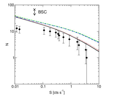
Figure 6: $\mathrm{Log\,N}$-$\mathrm{Log\,S}$ distribution for Model I. Four variants are shown: $\mathrm{R_{belt}}=500$ pc and truncated mass spectrum (full line), $\mathrm{R_{belt}}=500$ pc and non-truncated mass spectrum (dotted line), $\mathrm{R_{belt}}=300$ pc and truncated mass spectrum (dash-dotted line), and finally $\mathrm{R_{belt}}=300$ pc (dashed line) for non-truncated mass distribution.

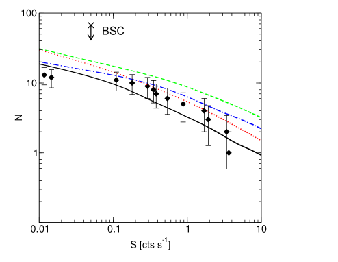
Figure 7: $\mathrm{Log\,N}$-$\mathrm{Log\,S}$ distribution for Model II. Line styles as in Fig. 6.

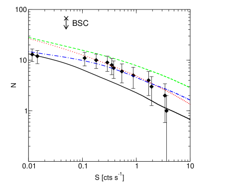
Figure 8: $\mathrm{Log\,N}$-$\mathrm{Log\,S}$ distribution for Model III. Line styles as in Fig. 6.

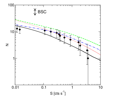
Figure 9: $\mathrm{Log\,N}$-$\mathrm{Log\,S}$ distribution for Model IV. Line styles as in Fig. 6.

For the case of the $\mathrm{Log\,N}$-$\mathrm{Log\,S}$ test we’d like to note that the value $\mathrm{R_{belt}}$=300 pc is more reliable. So, the Model I, for which at bright fluxes we see an overprediction of sources for this value of the Gould Belt radius, can be considered only as marginally passing the test. Other models do better. Especially, models III and IV. For them $\mathrm{Log\,N}$-$\mathrm{Log\,S}$ curves for $\mathrm{R_{belt}}=300$ pc match well the data points, leaving a room for few new possible identifications of close-by cooling NSs (active search is going on by different groups in France mo2005a ; mo2005b , in Germany bp2005 , in Italy Chieregato:2005es and in the USAag2005 ).

As in our $\mathrm{Log\,N}$-$\mathrm{Log\,S}$ calculations we use a particular mass spectrum in which there are nearly no objects with $M\stackrel{{\scriptstyle>}}{{\sim}}1.4$ - 1.5 $M_{\odot}$, we have a strong constraint on properties of a set of cooling curves which can satisfy all three tests. The position of the critical curve which devides hadronic stars from HyS is fixed by the chosen configuration. If curves for masses up to 1.4 $M_{\odot}$ lie too close to the critical one, then we overpredict the number of sources on the $\mathrm{Log\,N}$-$\mathrm{Log\,S}$ plot. If oppositely, we move curves for 1.3 -1.4 $M_{\odot}$ down (this is achieved by increasing the parameter $\alpha$ and thus making the density dependence of the X-gap steeper) then a narrow range of masses becomes responsible for a wide region in the $\mathrm{T}$ - $\mathrm{t}$ diagram.

A solution could be in changing the exponential dependence in Eq. 1 to the power-law. We plan to study this possibility in future.

The combined usage of all three tests can put additional constraints on the mass spectrum of compact objects. For example, if we look at Fig. 3 it is clear that small masses (M < 1.2 M_⊙) are necessary to explain hot objects with ages $\sim 10^{3}$ - $10^{4}$ yrs. If in such a case only a model with a truncated mass spectrum is able to explain the $\mathrm{Log\,N}$-$\mathrm{Log\,S}$ distribution of close-by NSs then the model is in trouble. On other hand, if an explanation of the $\mathrm{Log\,N}$-$\mathrm{Log\,S}$ deserves stars from low-mass bins, but cooling curves for these stars are in conradiction with the BC, then, again, the model has to be rejected.

In this series of our studies of the local population of cooling compact objects we use the mass spectrum which should fit to the solar neighbourhood enriched with stars from the mass range 8 - 15 $M_{\odot}$. Mass spectrum of all galactic newborn NSs can be different, but not dramatically. The number of low-mass stars ($\sim 1$ - $1.3\,M_{\odot}$) can be slightly decreased in favour of more massive stars. However, compact objects with $M\stackrel{{\scriptstyle<}}{{\sim}}1.5\,M_{\odot}$ anyway should significantly outnumber more massive objects. This claim has some observational support.

Unfortunately, a mass determination with high precision is available only for NSs in binary systems. Compact objects in X-ray binaries could accrete a significant amount of matter. Also mass determinations for them are much less precise than for radio pulsar systems. So, we concentrate on the latter. For some of the radio pulsars observed in binaries, accretion also played an important rôle. Without any doubts masses of millisecond pulsars do not represent their initial values. However, there is a small number of NSs with well determined masses, for which it is highly possible that these masses did not change significantly since these NSs were born (data on NS masses can be found, for example, in Manchester:2004bp ; cordes05 ; Lorimer:2005bw and references therein). These are secondary (younger) components of double NS systems. According to standard evolutionary scenarios these compact objects never accreted a significant amount of mass (as when they formed the primary component already was a NS). Their masses lie in the narrow range 1.18 - 1.39 $M_{\odot}$. Primary components of double NS binaries could accrete during their lifetime. However, this amount of accreted matter cannot be large as these are all high-mass binaries. Masses of these NSs are all below 1.45 $M_{\odot}$. This is also an important argument in favour of the statement that initial masses of most NSs are below $\sim 1.4$ - $1.5\,M_{\odot}$.

The recently discovered highly relativistic binary pulsar J1906+0746 Lorimer:2005un is the nineth example of such a system. The total mass is determined to be $2.61\pm 0.02\,M_{\odot}$. The pulsar itself is a young, not millisecond, object. It should not increase its mass due to accretion. So, we can assume that it is at least not heavier than the second - non-pulsar - component (we neglect here the possibility that the companion is a massive white dwarf, still this is a possibility), than we obtain that its mass is $\stackrel{{\scriptstyle<}}{{\sim}}1.3\,M_{\odot}$. Nine examples (without any counter-examples) is a very good evidence in favour of the mass spectrum used in our calculations. Of course, some effects of binary evolution can be important (for example, the mass of the core of a massive star can be influenced if the star looses part of its mass due to mass transfer to the primary companion or due to common envelope formation), and so for isolated stars (or stars in very wide binaries) the situation can be slightly different. However, with these observational estimates of initial masses of NSs we feel more confident using the spectrum with a small number of NSs with $M\stackrel{{\scriptstyle>}}{{\sim}}1.4$ - $1.5\,M_{\odot}$.

Brighter sources are easier to discover. So, among known cooling NSs the fraction of NSs with masses $1\,M_{\odot}\stackrel{{\scriptstyle<}}{{\sim}}M\stackrel{{\scriptstyle<}}{{\sim}}1.5\,M_{\odot}$ should be even higher than in the original mass spectrum. So, we have the impression that it is necessary to try to explain even cold (may be with an exception of 1-2 coldest) sources with $M\stackrel{{\scriptstyle<}}{{\sim}}1.4$ - $1.5\,M_{\odot}$. Especially, the Magnificent seven and other young close-by compact objects should be explained as most typical representatives of the whole NS population footnote . We want to underline that, even being selected by their observability in soft X-rays, these sources form one of the most uniform samples of young isolated NSs. In this sense, the situation as in Fig. 1 where a significant number of sources are explained by cooling curves corresponding to $1.5\,M_{\odot}\stackrel{{\scriptstyle<}}{{\sim}}M\stackrel{{\scriptstyle<}}{{\sim}}1.7\,M_{\odot}$ should be considered as a disadvantage of the model. Particularly, Vela, Geminga and RX J1856-3754 should not be explained as massive NSs. These all are young close-by sources, and the probability that so near-by we observe young NSs which come out of few percent of the most massive objects of this class is low.

All the above gives us the opportunity to formulate the conjecture of a mass spectrum constraint: data points should be explained mostly by NSs with typical masses. For all known data this typical means $1.1\,M_{\odot}\stackrel{{\scriptstyle<}}{{\sim}}M\stackrel{{\scriptstyle<}}{{\sim}}1.5\,M_{\odot}$.

The $\mathrm{Log\,N}$-$\mathrm{Log\,S}$ test is the only one that takes into account the mass spectrum explicitely. This is an additional argument in favour of using this test together with others.

Taking all together, we conclude that Model IV is the best among studied examples from the point of view of all three tests plus mass constraint.

VI Conclusion

We made a preliminary study of cooling curves for HyS based on the approach in Paper II which suggests that if quark matter occurs in a compact star, it has to be in the 2SC+X phase, where the hypothetical X-gap still lacks a microscopical explanation. All three tests of the cooling behavior ($\mathrm{Log\,N}$-$\mathrm{Log\,S}$, $\mathrm{T}$-$\mathrm{t}$, BC) are applied. Four models defined by the two-parameter ansatz for the X-gap were calculated. Model II with a density-independent X-gap could directly be excluded since it was not able to explain some cooling data including Vela at all. Two of the models (I and III) successfully passed two tests and marginally the third. None of these models could explain explain the temperature-age value for Vela within a typical mass range, i.e. for a Vela mass below 1.5 M_⊙. However, with a steeper density dependence of the X-gap than suggested in Paper II, we were able to fulfill all 4 constraints and exemplified this for model IV. To conclude, HyS with a 2SC+X quark matter core appear to be good candidates to explain the cooling behaviour of compact objects, although a consistent theoretical explanation of the hypothetical X-gap and its steep density dependence has still to be developed.

Model	$\Delta_{0}$ [MeV]	$\alpha$	BC	T – t	Log N – Log S	M${}_{\rm typ}\leq$ 1.5 M⊙	All tests
I	1	10	+	+	$\circ$	-	-
II	0.1	0	+	-	+	-	-
III	0.1	2	+	$\circ$	+	-	-
IV	5	25	+	+	+	+	+

Table 1: Parameter values $\Delta_{0}$ and $\alpha$ for Models I - IV defining the density dependence of the X-gap introduced in Eq. (1). The symbols +, - and $\circ$ denote whether or not a given model passes the proposed cooling tests, fails or is indifferent, respectively.