Solitons in relativistic mean field models

Abstract

Assuming that the nucleus can be treated as a perfect fluid we study the conditions for the formation and propagation of Korteweg-de Vries (KdV) solitons in nuclear matter. The KdV equation is obtained from the Euler and continuity equations in nonrelativistic hydrodynamics. The existence of these solitons depends on the nuclear equation of state, which, in our approach, comes from well known relativistic mean field models. We reexamine early works on nuclear solitons, replacing the old equations of state by new ones, based on QHD and on its variants. Our analysis suggests that KdV solitons may indeed be formed in the nucleus with a width which, in some cases, can be smaller than one fermi.

I Introduction

Understanding the nucleus and its properties in terms of QCD is a very ambitious goal and we are still far from it. Significant progress has been achieved in this direction with the use of chiral perturbation theory weise . On the other hand, relativistic mean field (RMF) models have been sucessfully used to describe the bulk properties of nuclear matter, finite nuclei and dense stars furn ; abcm ; lala ; serot . Although they are only effective models, they are simple, depend only on few parameters and are the ideal tool to test certain aspects of nuclear matter.

In this work we shall use the relativistic mean field model discussed in lala to investigate the formation and propagation of Korteveg - de Vries solitons in nuclear matter. Assuming that nuclear matter behaves like an ideal fluid we wish to know whether small baryon density perturbations can propagate without dissipation through the medium. If this turns out to be case, these pulses might be responsible for interesting phenomena. One of them would be the apparent nuclear transparency in proton nucleus collisions at low energies. The impinging proton would be absorbed by the fluid and turned into a density pulse. It would then be able to traverse the target nucleus emerging on the other side. This idea has been first advanced in frsw . In rawei the experimental evidence of this “nuclear transparency” was discussed. In rww the formalism was improved with the inclusion of viscosity and three-dimensional expansion. In hef the effect of the nuclear surface was considered. One important lesson from all these works is that the formation of solitons depends in a crucial way on the equation of state (EOS). In frsw ; rawei ; rww ; hef the equation of state employed was borrowed from glass and it was very phenomenological, containing no information about the microscopic nucleon dynamics.

The experimental signature of the nuclear soliton is very difficult to measure, since the outcoming nucleon emerges in a direction very close to the beam. Probably because of this reason the subject was left aside for almost ten years. Soliton formation in nuclear matter was then revived in abu , where a different equation of state was considered. This EOS was developed in vaut and was based on the nucleon-nucleon microscopic interaction given by the Skyrme force. The main finding of abu was that the nuclear soliton is not a compression pulse, as thought before. Instead, it is a rarefaction pulse due to a sign inversion appearing because of the use of Skyrme interactions.

Now, another ten years later, we come back to this subject because we feel that this beautiful idea has not been explored enough. We shall replace the EOS used in the early works by another one, based on the model of lala . The usual relativistic mean field models do not generate equations of state which lead to solitons because they do not contain higher derivatives, required in nonlinear differential equations. Therefore we will introduce a new interaction term in the Lagrangian of lala .

This work is organized as follows. In the next section we present some simple formulas of nonrelativistic hydrodynamics and write them in terms of the baryon and energy density. This will help to establish the connection between these equations and the relativistic mean field EOS. In the subsequent section we discuss the model of lala , introduce the new interaction term and, in the mean field approximation, derive the equation of state. In the following section, we combine the hydrodynamic equations with the new EOS and derive the KdV equation and its analytical solution. The last section contains some concluding remarks.

II Hydrodynamics

The basic equations of nonrelativistic hydrodynamics hidro are Euler equation

$${\frac{\partial\vec{v}}{\partial t}}+(\vec{v}\cdot\nabla)\vec{v}=-\bigg{(}{\frac{1}{\rho}}\bigg{)}\nabla p$$ (1)

and the continuity equation

$${\frac{\partial\rho}{\partial t}}+{{\nabla}}\cdot(\rho{\vec{v}})=0$$ (2)

In these equations, $\rho$ is the mass density, which, in the nuclear medium, is related to the baryon density through

$$\rho=M\rho_{B}$$ (3)

where $M$ is the nucleon mass. The enthalpy per nucleon is given by hidro :

$$dh=Tds+Vdp$$ (4)

where    $V=1/\rho_{B}$    is the specific volume. For a perfect fluid $(ds=0)$ the equation above becomes $dp=\rho_{B}dh$ and consequently:

$$\nabla p=\rho_{B}\nabla h$$ (5)

Inserting (3) and (5) in (1) and in (2) we obtain

$${\frac{\partial\vec{v}}{\partial t}}+(\vec{v}\cdot\nabla)\vec{v}=-\bigg{(}{\frac{1}{M}}\bigg{)}\nabla h$$ (6)

and

$${\frac{\partial\rho_{B}}{\partial t}}+{{\nabla}}\cdot(\rho_{B}{\vec{v}})=0$$ (7)

The enthalpy per nucleon may also be written as abu :

$$h=E+\rho_{B}{\frac{\partial E}{\partial\rho_{B}}}$$ (8)

where $E$ is the energy per nucleon given by:

$$E=\frac{\varepsilon}{\rho_{B}}$$ (9)

which inserted in (8) leads to:

$$h={\frac{\partial\varepsilon}{\partial\rho_{B}}}$$ (10)

and therefore:

$$\nabla h=\nabla{\frac{\partial\varepsilon}{\partial\rho_{B}}}$$ (11)

With these simple manipulations we can make explicit the dependence of Euler equation (6) on $\varepsilon(\rho_{B})$, or in other words, on the equation of state of nuclear matter.

As it will be seen later, it is possible to perform a combination of (6) and (7) in a specific way to obtain a nonlinear differential equation for the baryon density, with soliton solutions. The existence or not of these solitons depends on the function $\varepsilon(\rho_{B})$. A key feature of (6) and (11) is that they contain the gradient of the derivative of the energy density. If $\varepsilon$ contains a Laplacian of $\rho_{B}$, i.e.,

$${\mathcal{\varepsilon}}\propto...+...\nabla^{2}\rho_{B}+...$$ (12)

then equation (6) will have a cubic derivative with respect to the space coordinate, which will give rise to the Korteweg-de Vries equation for the density. The most popular RMF models do not have higher derivative terms and, even if they have at the start, these terms are usually neglected during the calculations. In the next section we show how to overcome these limitations and obtain a slightly more general expression for $\varepsilon(\rho_{B})$ with Laplacians.

III Modified QHD

We start with the well known variant of QHD-I serot , employed in lala :

$$\mathcal{L}_{0}=\bar{\psi}[\gamma_{\mu}(i\partial^{\mu}-g_{V}V^{\mu})-(M-g_{S}\phi)]\psi+{\frac{1}{2}}\Big{(}\partial_{\mu}\phi\partial^{\mu}\phi-{m_{S}}^{2}\phi^{2}\Big{)}$$

$$-{\frac{1}{4}}F_{\mu\nu}F^{\mu\nu}+{\frac{1}{2}}{m_{V}}^{2}V_{\mu}V^{\mu}-{\frac{b\phi^{3}}{3}}-{\frac{c\phi^{4}}{4}}$$ (13)

where, as usual, the degrees of freedom are the baryon field $\psi$, the neutral scalar meson field $\phi$ and the neutral vector meson field $V_{\mu}$, with the respective couplings and masses. The parameters $b$ and $c$ will be taken from lala . As it can be seen, there are no higher order derivatives. This is the reason why the traditional QHD and most of its numerous variants do not give an equation of state compatible with soliton propagation, like (12). For this it is necessary, in first place, to modify the Lagrangian, introducing a term with Laplacian derivative couplings. The simplest one is given by:

$${\mathcal{L_{M}}}\equiv{\frac{g_{V}}{{m_{V}}^{2}}}\bar{\psi}(\partial_{\nu}\partial^{\nu}V_{\mu})\gamma^{\mu}\psi$$ (14)

where the subscrit $\mathcal{M}$ denotes “modification” in QHD. First of all, this term is designed to be small in comparison with the main baryon - vector meson interaction term $g_{V}\bar{\psi}\gamma_{\mu}V^{\mu}\psi$. Because of the derivatives, it is of the order of:

$$\frac{p^{2}}{m_{V}^{2}}\sim\frac{k_{F}^{2}}{m_{V}^{2}}\sim 0.12$$ (15)

where the Fermi momentum is $k_{F}\simeq 0.28$ GeV and $m_{V}\simeq 0.8$ GeV. The form chosen for ${\mathcal{L_{M}}}$ is not dictated by any symmetry argument, has no other deep justification and is just one possible interaction term among many others cdmg . It is used here as a prototype. In the future, we plan to address this problem with a state of the art Lagrangian. As it can be immediately guessed, the integration by parts of ${\mathcal{L_{M}}}$ leads to a D’Alembertian acting on the baryon current. We present (14) with the derivatives acting on $V^{\mu}$ just because it can be more easily compared to $g_{V}\bar{\psi}\gamma_{\mu}V^{\mu}\psi$ it allows for estimates like (15). The total Lagrangian is then:

$${\mathcal{L}}=\mathcal{L}_{0}+\mathcal{L}_{M}$$ (16)

Integrating $\mathcal{L}_{M}$ by parts twice, making the standard mean field approximation

$$V_{\mu}\rightarrow<V_{\mu}>\equiv\delta_{\mu 0}V_{0}$$ (17)

$$\phi\rightarrow<\phi>\equiv\phi_{0}$$ (18)

and neglecting the time and spatial derivatives of the fields $V_{0}$ and $\phi_{0}$, we arrive at the approximate Lagrangian $\mathcal{L^{\prime}}$ given by:

$$\mathcal{L^{\prime}}=\bar{\psi}[(i\gamma_{\mu}\partial^{\mu}-g_{V}\gamma_{0}V_{0})-(M-g_{S}\phi_{0})]\psi-{\frac{1}{2}}{m_{S}}^{2}{\phi_{0}}^{2}+{\frac{1}{2}}{m_{V}}^{2}{V_{0}}^{2}$$

$$-{\frac{b{\phi_{0}}^{3}}{3}}-{\frac{c{\phi_{0}}^{4}}{4}}+{\frac{g_{V}}{{m_{V}}^{2}}}[\partial_{\nu}\partial^{\nu}(\bar{\psi}\gamma^{0}\psi)]V_{0}$$ (19)

The equations of motion of the fields are:

$$[(i\gamma_{\mu}\partial^{\mu}-g_{V}\gamma_{0}V_{0})-(M-g_{S}\phi_{0})]\psi=0$$ (20)

$${{m_{V}}^{2}}V_{0}=g_{V}\bar{\psi}\gamma^{0}\psi\,$$ (21)

$${m_{S}}^{2}\phi_{0}=g_{S}\bar{\psi}\psi-b{\phi_{0}}^{2}-c{\phi_{0}}^{3}$$ (22)

where, for simplicity, we have neglected the terms containing Laplacians. This means that the perturbation changes slightly the energy of the system, but does not affect the dynamics of the environment, i.e., of the unperturbed $\psi$, $\phi$ and $V^{\mu}$ fields. The energy density is calculated using the energy-momentum tensor:

$$\varepsilon=<T_{{0}{0}}>=-g_{00}\mathcal{L^{\prime}}+(\partial_{0}\psi){\frac{\partial\mathcal{L^{\prime}}}{\partial(\partial^{0}\psi)}}$$ (23)

which, with the help of (19), (20), (21) is given by:

$$\varepsilon={\frac{{g_{V}}^{2}}{2{m_{V}}^{2}}}\rho_{B}^{2}+{\frac{{m_{S}}^{2}}{2}}{\bigg{[}{\frac{(M^{*}-M)}{g_{S}}}\bigg{]}}^{2}+$$

$$+{\frac{\gamma}{(2\pi)^{3}}}\int_{0}^{k_{F}}d^{3}{k}({\vec{k}}^{2}+{M^{*}}^{2})^{1/2}+{\frac{b}{3g_{S}^{3}}}(M^{*}-M)^{3}+{\frac{c}{4g_{S}^{4}}}(M^{*}-M)^{4}$$

$$+{\frac{{g_{V}}^{2}}{{m_{V}}^{4}}}\rho_{B}\nabla^{2}\rho_{B}-{\frac{{g_{V}}^{2}}{{m_{V}}^{4}}}\rho_{B}\bigg{(}{\frac{\partial^{2}\rho_{B}}{\partial t^{2}}}\bigg{)}$$ (24)

where $(\gamma)$ is the baryon spin-isospin degeneracy factor and $M^{*}$ stands for the nucleon effective mass:

$$M^{*}\equiv M-g_{S}\phi_{0}$$

The two terms in the last line of (24) come from ${\mathcal{L_{M}}}$. Baryon number propagation in nuclear matter has been studied in shin with the help of the diffusion equation:

$${\frac{\partial\rho_{B}}{\partial t}}=D\,\nabla^{2}\rho_{B}$$ (25)

where the diffusion constant $D$ was numerically evaluated as a function of density and temperature and found to be $D\simeq\,0.35\,\,fm$ at densities comparable to the equilibrium nuclear density and temperatures of the order of $80$ MeV. The exact value of $D$ at $T=0$ is unknown but its dependence both with temperature and density is very smooth and an extrapolation to $T=0$ points to values even smaller than $0.35$ fm. This number is small compared to any nuclear size scale and can be interpreted as indicating that density gradients do not disappear very rapidly in nucler matter. Using (25) twice in the last term of (24) it can be rewritten as:

$$-{\frac{{g_{V}}^{2}}{{m_{V}}^{4}}}\rho_{B}\bigg{(}{\frac{\partial^{2}\rho_{B}}{\partial t^{2}}}\bigg{)}=-{\frac{{g_{V}}^{2}}{{m_{V}}^{4}}}\rho_{B}{\frac{\partial}{\partial t}}\bigg{(}D\nabla^{2}\rho_{B}\bigg{)}=-{\frac{{g_{V}}^{2}}{{m_{V}}^{4}}}\rho_{B}D^{2}[\nabla^{2}(\nabla^{2}\rho_{B})]$$ (26)

which, in the context of the present calculation, can be neglected because $\nabla^{2}(\nabla^{2}\rho_{B})<<(\nabla^{2}\rho_{B})$. With this last approximation, the final form of the energy density is given by (24) without the last term. The baryon density up to the Fermi level $(k_{F})$ is given by:

$$\psi^{\dagger}\psi\equiv\rho_{B}={\frac{\gamma({{k_{F}})^{3}}}{6\pi^{2}}}$$

As usual, the nucleon effective mass is determined by the minimization of $\varepsilon(M^{*})$ with respect to $M^{*}$, which results in the self-consistency relation:

$$M^{*}=M-{\frac{{g_{S}}^{2}}{{m_{S}}^{2}}}{\frac{\gamma}{(2\pi)^{3}}}\int^{k_{F}}_{0}d^{3}{k}{\frac{M^{*}}{\Big{(}{\vec{k}}^{2}+{M^{*}}^{2}\Big{)}^{1/2}}}$$

$$-{\frac{g_{S}^{2}}{ms^{2}}}\bigg{[}{\frac{b}{g_{S}^{3}}}(M^{*}-M)^{2}+{\frac{c}{g_{S}^{4}}}(M^{*}-M)^{3}\bigg{]}$$

The main result of this section is (24), which, in what follows, will be used in the derivation of the KdV equation. By keeping $\nabla^{2}\rho_{B}$ (but not $\nabla^{2}\nabla^{2}\rho_{B}$) we take into account the small inhomogeneities, which do not change rapidly in time (and therefore we neglect $\frac{\partial\rho_{B}}{\partial t}$). Whereas this approximation is quite often used at the nuclear surface, it is not very common for the bulk of nuclear matter. We believe, however, that it is quite reasonable.

IV The KdV solitons

In this section we follow the treatment developed in frsw and abu to obtain the Korteweg-de Vries equation in one dimension by the combination of (6) and (7).

Expression (24) is valid for any $\rho_{B}$. In order to make contact with the nuclear matter phenomenology and use the constraints imposed by the saturation curve, we will now use (24) to compute the energy per baryon $E$ (9). We then Taylor expand it around the equilibrium density $\rho_{0}$ up to second order:

$$E(\rho_{B})=E(\rho_{0})+\frac{1}{2}\bigg{(}{\frac{\partial^{2}E}{{\partial\rho_{B}}^{2}}}\bigg{)}_{\rho_{B}=\rho_{0}}(\rho_{B}-\rho_{0})^{2}$$ (27)

where the first order term vanishes because of the saturation condition

$${\frac{\partial}{{\partial\rho_{B}}}}\bigg{(}{\frac{\varepsilon}{\rho_{B}}}-M\bigg{)}_{\rho_{B}=\rho_{0}}\hskip 14.22636pt=\hskip 14.22636pt\bigg{(}{\frac{\partial E}{{\partial\rho_{B}}}}\bigg{)}_{\rho_{B}=\rho_{0}}\hskip 14.22636pt=\hskip 14.22636pt0$$

The derivative coefficient in (27) may be rewritten as abu :

$$\bigg{(}{\frac{\partial^{2}E}{{\partial\rho_{B}}^{2}}}\bigg{)}_{\rho_{B}=\rho_{0}}\,=\,\frac{M{c_{s}}^{2}}{\rho_{0}^{2}}$$

where $M$ is the nucleon mass and $c_{s}$ is the speed of sound in nuclear matter. Calculating the enthalpy per nucleon (8) by using (27) leads to:

$$h=E(\rho_{0})+{\frac{M{c_{s}}^{2}}{2{\rho_{0}}^{2}}}(3{\rho_{B}}^{2}+{\rho_{0}}^{2}-4{\rho_{B}}{\rho_{0}})$$ (28)

where

$$E(\rho_{0})=\bigg{(}{\frac{{g_{V}}^{2}}{2{m_{V}}^{2}}}\bigg{)}{\rho_{0}}+{\frac{\eta(\rho_{0})}{\rho_{0}}}+\bigg{(}{\frac{{g_{V}}^{2}}{{m_{V}}^{4}}}\bigg{)}(\nabla^{2}\rho_{B})$$ (29)

and

$$\eta(\rho_{0})\equiv{\frac{{m_{S}}^{2}}{2}}{\bigg{[}{\frac{(M^{*}-M)}{g_{S}}}\bigg{]}}^{2}+{\frac{\gamma}{(2\pi)^{3}}}\int_{0}^{k_{F}}d^{3}{k}({\vec{k}}^{2}+{M^{*}}^{2})^{1/2}+$$

$$+{\frac{b}{3g_{S}^{3}}}(M^{*}-M)^{3}+{\frac{c}{4g_{S}^{4}}}(M^{*}-M)^{4}$$

where the integration limit $k_{F}$ (which appears also in $M^{*}=M^{*}(k_{F})$) is fixed at the value corresponding to $\rho_{0}$. Inserting (28) in (6) we arrive at:

$${\frac{\partial\vec{v}}{\partial t}}+(\vec{v}\cdot\nabla)\vec{v}=-\bigg{(}{\frac{{c_{s}}^{2}}{2{\rho_{0}}^{2}}}\bigg{)}[6{\rho_{B}}(\nabla\rho_{B})-4{\rho_{0}}(\nabla{\rho_{B}})]$$

$$-\bigg{(}{\frac{{g_{V}}^{2}}{M{m_{V}}^{4}}}\bigg{)}\nabla(\nabla^{2}\rho_{B})$$ (30)

We now repeat the steps developed in frsw and abu , write (30) and (7) in one space dimension ($x$) and introduce dimensionless variables for the density and velocity:

$$\hat{\rho}={\frac{\rho_{B}}{\rho_{0}}}$$ (31)

and

$$\hat{v}={\frac{v}{c_{s}}}$$ (32)

We next define the “stretched coordinates” $\xi$ and $\tau$ as in frsw ; abu ; davidson :

$$\xi=\sigma^{1/2}{\frac{(x-{c_{s}}t)}{R}}$$ (33)

and

$$\tau=\sigma^{3/2}{\frac{{c_{s}}t}{R}}$$ (34)

where $R$ is a size scale and $\sigma$ is a small ($0<\sigma<1$) expansion parameter chosen to be davidson :

$${\sigma}={\frac{\mid u-{c_{s}}\mid}{{c_{s}}}}$$ (35)

where $u$ is the propagation speed of the perturbation. After these tedious but straightforward substitutions, we expand (31) and (32) around their equilibrium values:

$$\hat{\rho}=1+\sigma\rho_{1}+\sigma^{2}\rho_{2}+\dots$$ (36)

$$\hat{v}=\sigma v_{1}+\sigma^{2}v_{2}+\dots$$ (37)

Equations (30) and (7) will contain power series in $\sigma$ up to $\sigma^{2}$. Since the coefficients in these series are independent we get a set of equations, which, when combined, lead to the KdV equation for $\rho_{1}$

$${\frac{\partial{\rho}_{1}}{\partial\tau}}+3{{\rho}_{1}}{\frac{\partial{\rho}_{1}}{\partial\xi}}+\bigg{(}{\frac{{g_{V}}^{2}{\rho_{0}}}{2M{c_{s}}^{2}{m_{V}}^{4}R^{2}}}\bigg{)}{\frac{\partial^{3}{\rho}_{1}}{\partial\xi^{3}}}=0$$ (38)

which has a well known soliton solution. We may rewrite the above equation back in the $x\,-\,t$ space obtaining a KdV-like equation for ${\hat{\rho}_{1}}$ with the following solitonic solution:

$${\hat{\rho}_{1}}(x,t)={\frac{(u-{c_{s}})}{{c_{s}}}}sech^{2}\bigg{[}{\frac{{m_{V}}^{2}}{{g_{V}}}}\sqrt{{\frac{(u-{c_{s}}){c_{s}}M}{2{\rho_{0}}}}}(x-ut)\bigg{]}$$ (39)

where ${\hat{\rho}_{1}}\equiv\sigma{\rho_{1}}$. The solution above is a bump with width $\lambda$ given by:

$$\lambda={\frac{g_{V}}{{m_{V}}^{2}}}\sqrt{{\frac{2{\rho_{0}}}{(u-{c_{s}}){c_{s}}M}}}$$ (40)

Since

$$0<sech^{2}(\theta)\leq 1$$

and since

$${\frac{u-c_{s}}{c_{s}}}=\sigma\leq 1$$ (41)

we can see that ${\hat{\rho}_{1}}$ is always smaller than one and is consistent with the expansion (36). Relation (41) implies that $u\leq u_{max}=2c_{s}$. This upper bound is arbitrary, being a consequence of the choice (35), but it must exist. As mentioned in the introduction, the perturbation of the medium may be caused by the passage of a nucleon projectile and we expect that for higher projectile energies the modification of medium will be so strong that our perturbative approach will break down. The upper bound in the pulse velocity implies a limit for the momentum of the incident nucleon given by:

$$p_{max}={\frac{2c_{s}M}{{\sqrt{1-4{c_{s}}^{2}}}}}$$ (42)

As it can be seen from (40), the soliton width depends on parameters of the microscopic dynamics, as the coupling and mass which come from the Lagrangian (16). The sound velocity comes from the EOS derived from the same Lagrangian. The expression (40) also reveals the supersonic nature of this phenomenon, since it is only possible for $u>c_{s}$.

In the case where the density pulse is caused by a nucleon traversing a nucleus, if the width is comparable to the nucleon size and much smaller than the nuclear radius, the pulse will be localized and the impinging nucleon may emerge from the nucleus. If, on the other hand, $\lambda$ is large, of the order of the nuclear radius, then the incident energy will most likely be absorbed by the nucleus as a whole, which will undergo some collective excitation and decay.

In the numerical evaluation of (40) we need to know the values of the parameters appearing in the Lagrangians (13) and (14). For $\mathcal{L}_{0}$ we consider both the original QHD-I, without the nonlinear terms, just as a reference, and the most phenomenologically successful model of lala , with its different parameter choices labeled by $NL1$, $NL3$, $NL3-II$ and $NL-SH$. The use of the original QHD-I equation of state in hydrodynamical calculations leads to a too rapidly expanding system, as it was shown in mnno .

All the input numbers as well as the calculated incompressibilities $K$, equilibrium densities $\rho_{0}$, nucleon effective masses $M^{*}$ and sound velocities $c_{s}$ are shown in Table 1.

	$QHD$	$NL1$	$NL3$	$NL3-II$	$NL-SH$
K(MeV)	545	211	272	272	355
M(MeV)	939	938	939	939	939
$m_{S}(MeV)$	500	492	508,2	507,7	526
$m_{V}(MeV)$	780	783	782,5	781,9	783
$g_{S}$	8,7	10,14	10,22	10,2	10,4
$g_{V}$	11,62	13,28	12,87	12,8	12,9
$M^{*}/{M}$	0,56	0,57	0,6	0,59	0,6
${\rho_{0}}(fm^{-3})$	0,19	0,15	0,15	0,15	0,15
$b(fm^{-1})$	0	-12,17	-10,43	-10,4	-6,9
$c$	0	-36,26	-28,9	-28,9	-15,8
$c_{s}$	0,25	0,16	0,18	0,18	0,2

Table 1: input parameters and results for $K$, $M^{*}$, $\rho_{0}$ and $c_{s}$.

It is interesting to observe that the maximal momentum $p_{max}$ depends on $c_{s}$ and therefore will be different for different models.

Choosing values for $u$, from $c_{s}$ to $u_{max}$, and computing both $\lambda$ and $p$ up to $p_{max}$ for the different models, we obtain the curves shown in Fig. 1. As it can be seen, the width decreases with the projectile energy, as anticipated in raha . We can also see that, the stiffer is the equation of state, the wider is the window for soliton formation. At bombarding energies of a few hundred MeV the collisions are probably too violent and the departure from the initial equilibrium state is too large for the soliton picture to be true. At energies smaller than $200$ MeV, the width starts to be larger but still significantly smaller than the nuclear radius. Moreover, the choice of $g_{V}$ in (14) was just a first guess. The derivative coupling could be different and much weaker, leading to narrower solitons. As it appears now in (40) $\lambda$ is directly proportional to $g_{V}$. If the coupling would be half of the value used here, even the softest EOS ($NL1$) would lead to narrow solitons. After having established the connection between KdV solitons and relativistic mean field models, we can test other theories and other derivative couplings.

The observation of KdV solitons in nucleon-nucleus collisions was also discussed in clare , considering the exisiting experimental results at that time. Nowadays much more data are available and it might be interesting to look at them with the soliton picture in mind, searching for some unexpected transparency.

V Summary and conclusions

Assuming that RMF models give a satisfactory description of nuclear matter and finite nuclei and, also, that the nucleus can be treated as a perfect fluid, we have investigated the possibility of formation and propagation of Korteweg - de Vries solitons in nuclear matter. We have updated the early estimates of the soliton properties, using more reliable equations of state. In doing so we had to introduce in the Lagrangian a term with derivative coupling between the baryon and the vector meson fields. The term used here was the simplest one and with it we could already find KdV solitons, which have their properties (in particular the width) controled by the microscopic parameters of the underlying theory, such as masses and couplings. Whereas the quantitative results are not entirely conclusive, they suggest that KdV may indeed exist in nuclear matter. It is fair to say that the subject deserves further investigation. Finally we would like to mention that, during the last decade, due to the CERN-SPS and RHIC programs, hydrodynamics has experienced a great revival heinz ; hama and supersonic phenomena super were also brought back to explain recent RHIC data. Nonlinear effects, as those discussed here, may be relevant also in this context.

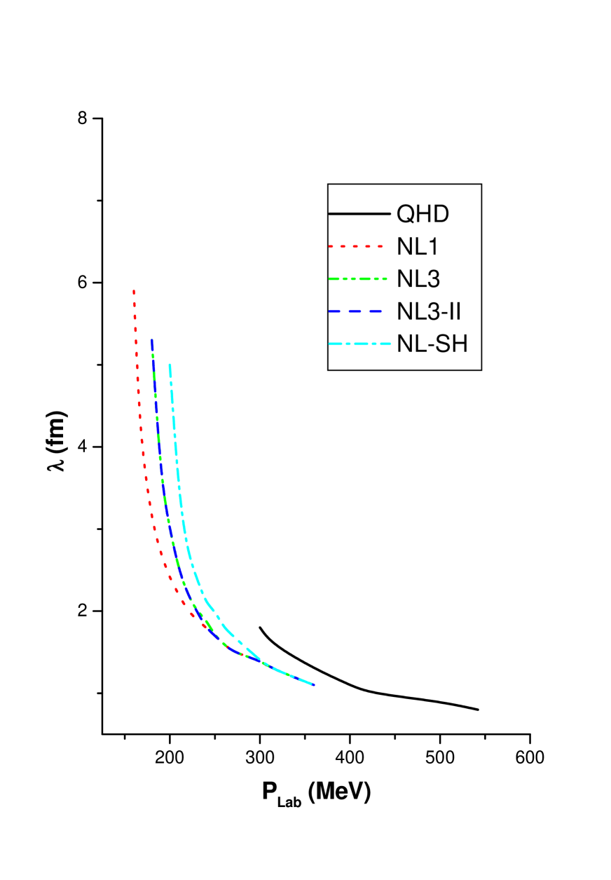
Figure 1: Soliton width as a function of the projectile momentum

- (1) W. Weise, Nucl. Phys. A751, 565 (2005); D. Vretenar, W. Weise, Lect. Notes Phys. 641, 65 (2004); S. Fritsch, N. Kaiser, W. Weise, Nucl. Phys. A750, 259 (2005); N. Kaiser, S. Fritsch, W. Weise, Nucl. Phys. A724, 47 (2003).
- (2) R.J. Furnstahl, Lect. Notes Phys. 641, 1 (2004); B.D. Serot, Int. J. Mod. Phys. A19S1, 107 (2004) and references therein.
- (3) S. S. Avancini, M. E. Bracco, M. Chiapparini and D. P. Menezes, J. Phys. G30, 27 (2004); Phys. Rev. C67, 024301 (2003); A. M. S. Santos and D. P. Menezes, Phys. Rev. C69, 045803 (2004).
- (4) G. A. Lalazissis, J. König and P. Ring, Phys. Rev. C55, 540 (1997).
- (5) B.D. Serot and J.D. Walecka, Advances in Nuclear Physics 16, 1 (1986).
- (6) G.N. Fowler, S. Raha, N. Stelte and R.M. Weiner, Phys. Lett. B115, 286 (1982).
- (7) S. Raha and R.M. Weiner, Phys. Rev. Lett. 50, 407 (1983).
- (8) S. Raha, K. Wehrberger and R.M. Weiner, Nucl. Phys. A433, 427 (1984).
- (9) E.F. Hefter, S. Raha and R.M. Weiner, Phys. Rev. C32, 2201 (1985).
- (10) A.E. Glassgold, W. Heckrotte and K.M. Watson, Ann. Phys. (N.Y.) 6, 1 (1959).
- (11) A.Y. Abul-Magd, I. El-Taher and F.M. Khaliel, Phys. Rev. C45, 448 (1992).
- (12) D. Vautherin and D. Brink, Phys. Rev. C5, 626 (1972).
- (13) L. Landau and E. Lifchitz, “Fluid Mechanics”, Pergamon Press, Oxford, (1987).
- (14) See, for example, M. Chiapparini, A. Delfino, M. Malheiro and A. Gattone, Z. Phys. A357, 47 (1997); A. Delfino, M. Chiapparini, M. Malheiro, L. V. Belvedere and A. O. Gattone, Z. Phys. A355, 145 (1996).
- (15) N. Sasaki, O. Miyamura, S. Muroya, C. Nonaka, Europhys. Lett. 54, 38 (2001); Phys. Rev. C62, 011901 (2000).
- (16) R.C. Davidson, “Methods in Nonlinear Plasma Theory”, Academic Press, New York an London, 1972.
- (17) D. P. Menezes, F. S. Navarra, M. Nielsen and U. Ornik, Phys. Rev. C47, 2635 (1993).
- (18) S. Raha, “Proceedings of the Fisrt International Workshop on Local Equilibrium in Strong Interaction Physics”, LESIP I, Bad Honnef 1984, Editors: D.K. Scott and R. Weiner, World Scientific, Singapore, (1984) p. 220.
- (19) R.B. Clare and D. Strottman, Phys. Rept. 141, 177 (1986).
- (20) U. Heinz, J. Phys. G31, S717 (2005); for a recent review see P.F. Kolb, U. Heinz, in “Quark Gluon Plasma 3”, Editors: R.C. Hwa and X.-N. Wang, World Scientific, Singapore, (2003) p. 634; nucl-th/0305084.
- (21) Y. Hama, T. Kodama and O. Socolowski Jr., Braz. J. Phys. 35, 24 (2005); Y. Hama and F. S. Navarra, Phys. Lett. B129, 251 (1984); Z. Phys. C26, 465 (1984); Z. Phys. C53, 501 (1992).
- (22) T. Renk and J. Ruppert, hep-ph/0509036; I. M. Dremin, hep-ph/0507167; L. M. Satarov, H. Stoecker and I. N. Mishustin, Phys. Lett. B627, 64 (2005).