Abstract

In ultrarelativistic heavy ion collisions a finite size QCD medium is created. In this paper we compute radiative energy loss to zeroth order in opacity by taking into account finite size effects. Transition radiation occurs on the boundary between the finite size medium and the vacuum, and we show that it lowers the difference between medium and vacuum zeroth order radiative energy loss relative to the infinite size medium case. Further, in all previous computations of light parton radiation to zeroth order in opacity, there was a divergence caused by the fact that the energy loss is infinite in the vacuum and finite in the QCD medium. We show that this infinite discontinuity is naturally regulated by including the transition radiation.

1 Introduction

The suppression pattern of high transverse momentum hadrons is considered to be a powerful tool to map out the density of the produced QCD plasma [1]-[3]. This suppression (so called jet quenching) is assumed to be mainly due to the medium induced radiative energy loss of high energy partons propagating through ultra-dense QCD matter [4]-[7]. However, even if final state multiple elastic and inelastic interactions are neglected, the difference between medium and the vacuum $0^{th}$ order energy loss would still be significant. This is due to the fact that the gluon dispersion relation is different in the medium and the vacuum, leading to differences in the associated $0^{th}$ order radiation. This effect was first pointed out by Ter-Mikayelian [8, 9], who considered the QED plasma case. In [10, 11] we developed a non-abelian QCD analog of the Ter-Mikayelian plasmon effect for the case of heavy quarks. We showed that while the Ter-Mikayelian effect is negligible for bottom quarks, it has an important effect on charm quarks, since it leads to a significant reduction of the vacuum radiation. This result is a consequence of the fact that the gluons in the QCD medium acquire a finite mass proportional to the temperature of the medium.

The computation presented in [10] was done under the assumption of an infinite QCD medium. This raises the question how to generalize these results to the more realistic case of a finite size QCD medium created in ultra-relativistic heavy ion collisions (URHIC). How the results from [10] will be modified by finite size QCD effects is the first goal of this paper.

Further, it is well known that light parton $0^{th}$ order energy loss is not infrared safe, i.e. it goes to infinity when the parton mass goes to zero. This infrared divergence is absorbed in the DGLAP evolution [12], so that the only part which contributes to the jet quenching is the difference between medium and vacuum energy loss. Since all previous computations [4, 7] assumed that the light quarks and gluons have the same zero mass in both the medium and the vacuum, the difference between medium and vacuum energy loss was found to be finite.

However, with the introduction of the Ter-Mikayelian effect, the finite parton mass in the medium regulates the infrared divergence of the $0^{th}$ order energy loss in the medium, while the corresponding energy loss in the vacuum remains infinite. This leads to the question how to regulate this discontinuity between medium and vacuum light parton energy losses. The second goal of this paper is to show how transition radiation naturally solves this problem.

The outline of the paper is as follows. In Section 2, we will compute the $0^{th}$ order radiation in a finite size QCD medium for both light and heavy quarks. For charm quarks we will show that the transition radiation lowers the Ter-Mikayelian effect from $30\%$ [10] to $15-20\%$. Additionally, we will show that for light partons the transition radiation naturally regulates the infinite discontinuity between $0^{th}$ order medium and the vacuum radiative energy loss. In Section 3, we will study how the difference between medium and the vacuum $0^{th}$ order energy loss depends on where the particle is produced. We will show that the difference between medium and vacuum $0^{th}$ order energy loss is positive (as intuitively expected) as long as the probe is produced far outside the medium (QED case). However, if the particle is produced inside the medium, such as in the QCD case, we will obtain that this naive expectation may not hold. In Section 4, we will extend our study from Sections 2 and 3 to include the fact that due to the confinement in the vacuum, the gluons may acquire finite mass. We will obtain qualitatively different results, compared to those presented in Sections 2 and 3, if the gluon mass in the vacuum is larger than in the medium. In Section 5, we will combine the results presented in Sections 2 and 4 with the medium induced radiative energy loss [13]. We find that for certain realistic values of the gluon mass in the vacuum, the light quarks can leave the $L<3$ fm medium essentially unquenched. We argue that the results presented in the Section 5 may provide us with a hint toward solving the puzzle posed by [14]. Finally, in Section 6 we summarize our results and put our work in the context of future research.

2 The one gluon $0^{th}$ order radiation in a finite size QCD medium

The aim of this section is to compute the $0^{th}$ order radiative energy loss when the parton is produced in a finite size dielectric medium. To introduce the finite size medium, we start from the approach described in [15]. As in [15], we consider the static medium of size $L$, and define two gluon masses, $m_{g,v}$ (for gluon radiated in the vacuum), and $m_{g,p}$ (for gluon radiated in the medium). We also assume that, in general, the running coupling constant can be different in the vacuum and in QGP. However, contrary to [15], we ignore spin effects, since they are irrelevant in the soft radiation limit that we consider in this paper.

To compute the $0^{th}$ order radiative energy loss in a finite QCD medium, we have to compute the squared amplitude of a Feynman diagram, $M^{rad}$. The Feynman diagram represents the source $J$, which at time ${\mbox{x}_{0}}$ produces an off-shell jet with momentum $p^{\prime}$ and subsequently (at ${\mbox{x}_{1}}>{\mbox{x}_{0}}$) radiates a gluon with momentum $k$. The jet emerges with momentum $p$ and mass $M$. We neglect the thermal shifts of the quark mass since 1) for heavy quarks, thermal effects on the quark mass are negligible, and 2) light quarks will be treated as massless particles for the reason explained in footnote 2.

The matrix element for this $0^{th}$ order in opacity radiation process can then be written in the following form

$$M^{rad}=\int d^{4}{\mbox{x}_{0}}\;J({\mbox{x}_{0}})\;d^{4}{\mbox{x}_{1}}\;\Delta_{M}({\mbox{x}_{1}}-{\mbox{x}_{0}})\;v^{\mu}({\mbox{x}_{1}})\;A_{\mu}^{\dagger}({\mbox{x}_{1}})\Phi^{\dagger}({\mbox{x}_{1}})$$ (1)

where $\Phi({\mbox{x}_{1}})=e^{-ip{\mbox{\scriptsize x}}}$ is the wave function of the final quark with (on-shell) momentum $p$ and $A_{\mu}({\mbox{x}_{1}})$ is the wave function of the emitted gluon. Vertex function $v^{\mu}({\mbox{x}_{1}})$ is given by $v^{\mu}({\mbox{x}_{1}})=g({\mbox{x}_{1}})(\overleftarrow{\partial}^{\mu}-\overrightarrow{\partial}^{\mu})$, where $g({\mbox{x}_{1}})$ is the running coupling constant which is in general different in the medium than in the vacuum.

For this problem it is convenient to use light cone coordinates [16]. This coordinate system is appropriate for systems moving with almost the speed of light. It is obtained by choosing new space-time coordinates $[{\mbox{x}^{+}},{\mbox{x}^{-}},{\bf x}]$, related to the coordinates in the laboratory frame $(t,z,{\bf x})$ by (${\bf x}$ is the transverse coordinate)

$${\mbox{x}}^{+}=(t+z)\,,\hskip 56.9055pt{\mbox{x}}^{-}=(t-z).$$ (2)

In the same way the light cone momentum $[p^{+},p^{-},{\bf p}]$ is related to the momentum in the laboratory frame $[E,p_{z},{\bf p}]$ by (${\bf p}$ is the transverse momentum)

$$p^{+}=(E+p_{z})\,,\hskip 56.9055ptp^{-}=(E-p_{z}).$$ (3)

Additionally, it can be shown that in the light cone coordinate system the propagator $\Delta_{M}({\mbox{x}})$ reduces to (see [16]):

$$\Delta_{M}({\mbox{x}})=\frac{-i}{(2\pi)^{3}}\int\frac{dp^{\prime+}d^{2}{\bf p^{\prime}}}{2p^{\prime+}}(\theta({\mbox{x}}^{+})e^{-ip^{\prime}{\mbox{\scriptsize x}}}+\theta(-{\mbox{x}}^{+})e^{ip^{\prime}{\mbox{\scriptsize x}}}),$$ (4)

where $p^{\prime-}\equiv\frac{{\bf p^{\prime}}^{2}+M^{2}}{p^{\prime+}}$.

In the spinless case, the wave function of the emitted gluon with momentum $k$ can be written as

$$A_{\mu}(x)=\epsilon_{\mu}(k)\;\Phi_{g}({\mbox{x}})\;c,$$ (5)

where $\epsilon(k)=[0,2\frac{{\mbox{\scriptsize{\boldmath$\epsilon$}}}{\bf\cdot k}}{k^{+}},{\mbox{\scriptsize{\boldmath$\epsilon$}}}]$ is the transverse polarization and $c$ is the color factor of the radiated gluon.

$$\Phi_{g}({\mbox{x}})=e^{-i\frac{1}{2}[k^{+}{\mbox{\scriptsize x}^{-}}+\int\limits_{0}^{\mbox{\scriptsize x}^{+}}d\xi\,k^{-}(\xi)]+i{\bf k\cdot x}}$$ (6)

is the wave function (derived in Appendix A) that satisfies the Klein-Gordon equation with position dependent gluon mass $m_{g}({\mbox{x}^{+}})$, and $k^{-}({\mbox{x}^{+}})=\frac{{\bf k}^{2}+m_{g}^{2}({\mbox{\scriptsize x}^{+}})}{k^{+}}$. In the static approximation $m_{g}({\mbox{x}^{+}})$ becomes

$$m_{g}({\mbox{x}^{+}})=m_{g,p}\;\theta(L-\frac{{\mbox{x}^{+}}}{2})+m_{g,v}\;\theta(\frac{{\mbox{x}^{+}}}{2}-L)\;,$$ (7)

where $m_{g,p}$ is gluon mass for the gluon radiated in the medium, while $m_{g,v}$ is gluon mass for the gluon radiated in the vacuum.

We can now compute $M_{rad}$ by substituting Eqs. (4)-(7) in Eq.(1), which leads to the fallowing result (see Appendix B for detailed calculation of $M_{rad}$):

$$M_{rad}=-2i\,J(p+k)\frac{{\mbox{\boldmath$\epsilon$}}{\bf\cdot k}}{x}\left[\frac{g_{p}}{p^{\prime+}}\frac{1-e^{i\chi_{p}L}}{\chi_{p}}+\frac{g_{v}}{p^{\prime+}}\frac{e^{i\chi_{p}L}}{\chi_{v}}\right]c\;,$$ (8)

where $g_{p}$ ($g_{v}$) is the running coupling constant in the medium (vacuum). The variable $x$ is defined as $x\equiv\frac{k^{+}}{p^{\prime+}}$ and

$$\chi_{v} = \frac{{\bf k}^{2}+M^{2}x^{2}+m_{g,v}^{2}}{xp^{\prime+}}\;,$$

$$\chi_{p} = \frac{{\bf k}^{2}+M^{2}x^{2}+m_{g,p}^{2}}{xp^{\prime+}}\;.$$ (9)

Here, we use for the initial quark a plane wave state in the ${\bf x}$-plane and set ${\bf p^{\prime}}=0$. Then ${\bf p}=-{\bf k}$, $p^{\prime-}=\frac{M^{2}}{p^{\prime+}}$ and $p^{-}=\frac{{\bf k}^{2}+M^{2}}{(1-x)p^{\prime+}}$. Note that soft radiation is defined as $x\ll 1$ (i.e. $p^{+}\gg k^{+}$), so we assume that $1-x\approx 1$. Additionally, as in [17], we assume that $J$ varies slowly with $p$, so that $J(p+k)\approx J(p)$.

In soft gluon approximation, the spectrum can be extracted from Eq. (8) as (see [17])

$$|M_{rad}^{0}|^{2}\frac{d^{3}\vec{{\bf p}}}{2E(2\pi)^{3}}\frac{d^{3}\vec{{\bf k}}}{2\omega(2\pi)^{3}}\approx d^{3}N_{J}\;d^{3}N_{g}^{(0)}\;\;,$$ (10)

where

$$d^{3}N_{J}=d_{R}|J(p)|^{2}\frac{d^{3}\vec{\mathbf{p}}}{(2\pi)^{3}2p^{0}}\;\;.$$ (11)

Here $d_{R}=3$ (for three dimensional representation of the quarks).

Finally, by using Eqs. (10, 11) together with Eq. (8) we obtain the main order fractional energy loss $(I\equiv\Delta E/E)$ for massive quarks and gluons in the QCD medium of finite size L

$$\frac{dI_{med}^{(0)}}{dx\;d^{2}{\bf k}} = \frac{dI_{vac}^{(0)}}{dx\;d^{2}{\bf k}}+2\frac{C_{R}{\bf k}^{2}}{\pi^{2}(p^{\prime+})^{2}}\frac{\sqrt{\alpha_{S}^{p}(k)}}{\chi_{p}}\left(\frac{\sqrt{\alpha_{S}^{p}(k)}}{\chi_{p}}-\frac{\sqrt{\alpha_{S}^{v}(k)}}{\chi_{v}}\right)(1-\cos(\chi_{p}L))$$ (12)

$$\xrightarrow{\alpha_{S}^{p}=\alpha_{S}^{v}} \frac{dI_{vac}^{(0)}}{dx\;d^{2}{\bf k}}+2\frac{C_{R}\alpha_{S}}{\pi^{2}}\frac{{\bf k}^{2}(m_{g,v}^{2}-m_{g,p}^{2})}{({\bf k}^{2}+m_{g,p}^{2}+M^{2}x^{2})^{2}({\bf k}^{2}+m_{g,v}^{2}+M^{2}x^{2})}$$

$$\hskip 85.35826pt\times(1-\cos(\frac{({\mbox{{\bf k}}}^{2}+m_{g,p}^{2}+M^{2}x^{2})L}{2Ex})),$$

where $\alpha_{S}^{p}(k)$ ($\alpha_{S}^{v}(k)$) is the running coupling constant in the medium (vacuum). $C_{R}$ is the color Casimir for the partons, i.e. $C_{R}=4/3$ for quarks and $C_{R}=3$ for gluons. $E$ is the initial jet energy. The second equation in (12) is valid in the $\alpha_{S}^{p}(k)=\alpha_{S}^{v}(k)$ case, where the physical meaning of the obtained results are more evident.

$I_{v}^{(0)}$ is $0^{th}$ order in opacity fractional energy loss in the vacuum:

$$\frac{dI_{vac}^{(0)}}{dx\;d^{2}{\bf k}}=\frac{C_{R}\alpha_{S}^{v}(k)}{\pi^{2}}\frac{{\bf k}^{2}}{({\bf k}^{2}+m_{g,v}^{2}+M^{2}x^{2})^{2}}\;$$ (13)

and $I_{med}^{(0)}$ is total $0^{th}$ order in opacity fractional energy loss in finite size medium, given by

$$I_{med}^{(0)}=I_{TM}^{(0)}+I_{trans}^{(0)}\;.$$ (14)

Here, $I_{TM}^{(0)}$ is the $0^{th}$ order in opacity fractional energy loss in the infinite size medium, which can be obtained from $I_{vac}^{(0)}$ by replacing $m_{g,v}$ by $m_{g,p}$ in Eq. (13). $I_{trans}^{(0)}$ is the additional transition radiation occurring when the jet is traversing from the medium to the vacuum. As a crosscheck, we note that, by neglecting spin effects in [15], Eq. (9) from [15] can be reduced to the Eq. (12) above. We note that the computation in [15] was done in 3-dimensional coordinate space ($z$, x), while our computations were more consistently performed in the light-cone 4-dimensional coordinate space.

To obtain the fractional energy losses, we perform the integration by using $0<|{\bf k}|<2x(1-x)E$, i.e. in our computations we do not introduce a lower momentum cutoff. For running coupling we use the ”Frozen $\alpha$ model” [18]

$$\alpha_{S}(Q^{2}-M^{2})={\rm Min}\{0.5,\frac{4\pi}{\beta_{0}Log(\frac{Q^{2}-M^{2}}{\Lambda_{QCD}^{2}})}\}={\rm Min}\{0.5,\frac{4\pi}{\beta_{0}Log(\frac{{\bf k}^{2}+m_{g}^{2}+M^{2}x^{2}}{x\Lambda_{QCD}^{2}})}\}\ \;\;\;,$$ (15)

where $\beta_{0}=\frac{28}{3}$ for effective number of flavors $n_{f}\approx 2.5$, $\Lambda_{QCD}\approx 0.2$ GeV, and $Q^{2}-M^{2}=\frac{{\bf k}^{2}+m_{g}^{2}+M^{2}x^{2}}{x}$. Note that $\alpha_{S}^{p}$ ($\alpha_{S}^{v}$) is obtained by setting $m_{g}^{2}=m_{g,p}^{2}$ ($m_{g}^{2}=m_{g,v}^{2}$) in Eq. (15).

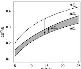
Figure 1: The reduction of the fractional $0^{th}$ order energy loss for charm quarks due to both the QCD Ter-Mikayelian effect and transition radiation is shown as a function of the quark energy. The dashed-dotted curve shows the vacuum energy loss if gluons are treated as massless and transversely polarized. Dashed curve shows the effect using the Ter-Mikayelian effect only, and solid curve shows the total effect by including both the Ter-Mikayelian effect and transition radiation. Assumed thickness of the medium is $L=5$ fm, charm mass is $M=1.5$ GeV and the gluon mass is $m_{g,v}=0$ GeV ($m_{g,p}=0.35$ GeV) for the vacuum (medium) case.

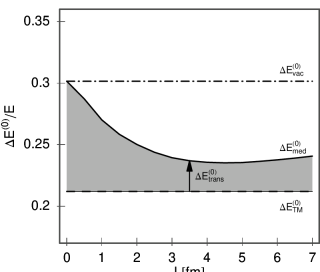
Figure 2: The reduction of the fractional $0^{th}$ order energy loss for $10$ GeV charm jet due to both the QCD Ter-Mikayelian effect and transition radiation is shown as a function of the thickness of the medium. The dashed-dotted curve shows the vacuum energy loss if gluons are treated as massless and transversely polarized. Dashed curve shows the effect using the Ter-Mikayelian effect only, and solid curve shows the total effect by including both the Ter-Mikayelian effect and transition radiation. We assume that the mass of the charm jet is $M=1.5$ GeV and the gluon mass is $m_{g,v}=0$ GeV ($m_{g,p}=0.35$ GeV) for the vacuum (medium) case.

We next use Eqs. (12)-(15) to provide a comprehensive analysis of the influence of the transition radiation to the total $0^{th}$ order in opacity energy loss for both light and heavy quarks. We first concentrate on the charm quark case and look how the $0^{th}$ order energy loss depend on the initial jet energy (Fig. 1) and thickness of the medium (Fig. 2). In Fig. 1 we see that for charm quarks, transition radiation lowers the Ter-Mikayelian effect from $30\%$ to $15-20\%$ for $L=5$ fm medium. In Fig. 2 we see that for a medium thickness greater than 4 fm the transition radiation becomes approximately independent of the thickness of the medium.

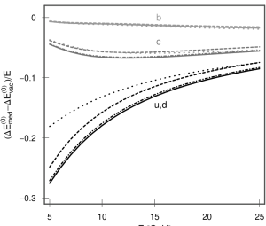
Figure 3: The difference between medium and the vacuum $0^{th}$ order fractional energy loss for light (the lower four curves), charm (the middle four curves) and bottom quarks (the upper four curves) is shown as a function of initial jet energy. Solid curves are computed by assuming running coupling given by Eq. (15), with different $\alpha_{S}^{p}$ in the medium and $\alpha_{S}^{v}$ in the vacuum. Dashed, dot-dashed and dotted curves are computed by assuming the same coupling constant both in the medium and in the vacuum. For dashed (dot-dashed) curves we used running coupling $\alpha_{S}^{p}$ ($\alpha_{S}^{v}$) given by Eq. (15). Dotted curves are computed by assuming constant coupling $\alpha_{S}=0.3$. Assumed thickness of the medium is $L=5$ fm, light quark mass is $M=0$ GeV, charm mass $M=1.5$ GeV, and bottom mass $M=4.5$ GeV. The gluon mass is $m_{g,v}=0$ GeV ($m_{g,p}=0.35$ GeV) for the vacuum (medium) case.

The previous two figures were computed by assuming running coupling (given by Eq. (15)) which is different in the medium and in the vacuum. In Fig. 3 we want to test how the obtained medium and the vacuum fractional energy loss difference ($I_{med}^{(0)}-I_{vac}^{(0)}$) is robust against variations in the choice of coupling constant. To do that, we plot $I_{med}^{(0)}-I_{vac}^{(0)}$ as a function of initial jet energy for three different choices of running coupling as well as constant coupling $\alpha_{S}=0.3$. We see that for heavy ($c$ and $b$) quarks, the difference between medium and the vacuum energy loss is almost independent on the choice of coupling constant. For the light quark case, we see that while $I_{med}^{(0)}-I_{vac}^{(0)}$ is robust to the choice of running coupling, it is fairly sensitive to the choice between running and constant coupling. For example, in $p_{\perp}<10$ GeV range, $30\%$ smaller $I_{med}^{(0)}-I_{vac}^{(0)}$ is obtained when constant coupling $\alpha_{S}=0.3$ is employed.

Additionally, from Fig. 3 we see that the finite mass (a.k.a. dead cone [19]) effect on $I_{med}^{(0)}-I_{vac}^{(0)}$ is strong, i.e. we see a qualitative difference between light and heavy quark $0^{th}$ energy losses, which persists at high momentum. For example, while $I_{med}^{(0)}-I_{vac}^{(0)}$ for light quarks is large and shows a noticeable dependence on jet energy, it is negligible for bottom quarks in the whole jet energy range.

The most striking observation from Fig. 3 is that, for the light quark case, the difference between medium and the vacuum energy loss ($I_{med}^{(0)}-I_{vac}^{(0)}$) is finite. To validate this numerical result analytically, we assume a perturbative vacuum (i.e. $m_{g,v}=0$ GeV) and the same coupling in the medium and in the vacuum (i.e. $\alpha_{S}^{p}=\alpha_{S}^{v}$). In the ($M=0$ GeV) light quark case, the Eq. (12) reduces to

$$\frac{d(I_{med}^{(0)}-I_{vac}^{(0)})}{dx\;d^{2}{\bf k}}=-2\frac{C_{R}\alpha_{S}}{\pi^{2}}\frac{m_{g,p}^{2}}{({\bf k}^{2}+m_{g,p}^{2})^{2}}\left(1-\cos(\frac{({\mbox{{\bf k}}}^{2}+m_{g,p}^{2})L}{2Ex})\right),$$ (16)

This equation is infrared safe when ${\bf k}\rightarrow 0$. This is an important result having in mind that without transition radiation, the Ter-Mikayelian effect leads to a discontinuity between finite medium and infinite vacuum energy loss. Therefore, we conclude that the transition radiation has special importance in the case of the light quarks since it provides a natural regularization of medium dispersion effects.

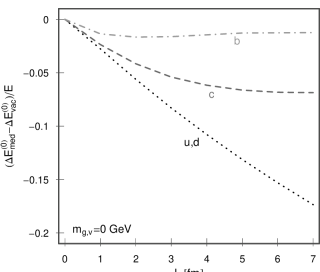
Figure 4: The difference between medium and the vacuum $0^{th}$ order fractional energy loss for light (dotted curve), charm (dashed curve) and bottom quark (dot-dashed curve) is shown as a function of the thickness of the medium. The initial jet energy is $E=15$ GeV. The curves were computed by assuming running coupling given by Eq. (15), with different coupling in the medium and in the vacuum. Light quark mass is $M=0$ GeV, charm mass $M=1.5$ GeV, and bottom mass $M=4.5$ GeV. The gluon mass is $m_{g,v}=0$ GeV ($m_{g,p}=0.35$ GeV) for the vacuum (medium) case.

In Fig. 4 we fix the energy jet to $15$ GeV, and test how the $I_{med}^{(0)}-I_{vac}^{(0)}$ depends on $L$ for different types of quarks. We see that light and heavy quarks show significantly different thickness dependence. For heavy quarks, $I_{med}^{(0)}-I_{vac}^{(0)}$ saturate after some value of $L$ (i.e. after $L=4$ fm for charm and $L=1$ fm for bottom). This saturation behavior is expected having in mind that for massive quarks and large enough $L$, $\cos(\chi_{p}L)$ becomes rapidly oscillating function. Then $\left\langle\cos(\chi_{p}L)\right\rangle\rightarrow 0$, and Eq. (12) becomes independent on the thickness of the medium. For the light quarks, we see that $|I_{med}^{(0)}-I_{vac}^{(0)}|$ increases approximately linearly with $L$. This linear thickness dependence persists for higher jet energies as well (results now shown). This result is unexpected, having in mind that, in the light quark case and $L/E\rightarrow 0$ limit, by expanding cosine in Eq. (16), we expect to obtain quadratic ($L^{2}$) thickness dependence for $I_{med}^{(0)}-I_{vac}^{(0)}$. However, by integrating Eq. (16) in the $L/E\rightarrow 0$ limit (and without expanding cosine) we obtain a result which depends linearly on the thickness $L$ of the medium (in agreement with the numerical results shown in Fig. 4):

$$I_{med}^{(0)}-I_{vac}^{(0)}\approx\frac{C_{R}\alpha_{S}}{2}\frac{m_{g,p}^{2}L}{E}\ln[\frac{E}{2m_{g,p}}].$$ (17)

Finally, from Figs. 1-4 we see that the total energy loss in the medium is smaller than in the vacuum. This result comes from Eq. (12), where we see that $\Delta E_{p}^{(0)}-\Delta E_{v}^{(0)}\propto(m_{g,v}^{2}-m_{g,p}^{2})$. Therefore, if the gluon mass in the medium is larger than in the vacuum, then the total $0^{th}$ order energy loss in the medium will be smaller than in the vacuum. Though mathematically correct, this result seems surprising, since it would be expected that the radiation in the medium (even at the lowest order) is always larger than the corresponding radiation in the vacuum, particularly having in mind the work presented in [9, 20]. In [9, 20] the transition radiation was studied for the particle traversing the QED medium, and it was shown that the lowest order radiative energy loss in the medium is always larger than in the vacuum. This study considered the case when the particle is produced outside the medium (at $z_{0}=-\infty$). However, contrary to the usual experiments involving a QED medium, where the medium is probed by using test particles produced far outside the medium, in URHIC the probes are produced inside the medium. Therefore, to be able to intuitively understand the result obtained from Eq. (12), we have to take into account the qualitative change in the experimental approaches between QED and QCD. In the next Section we study how the difference between medium and the vacuum energy loss depends on the point of particle production.

3 Dependence of the $0^{th}$ order energy loss on the point of particle production

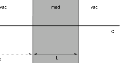
Figure 5: An illustration of the system studied in this Section. Gray area shows the medium of thickness $L$. Probe is produced in the vacuum at distance $|l_{0}|$ from the medium.

To study this particular problem we assume the static system shown in Fig. 5. That is, we consider the probe produced in the vacuum at the finite distance $l_{0}$ (i.e. ${\mbox{x}}_{0}^{+}=-2l_{0}<0$) from the medium of size $L$. As in the previous section, we assume that a gluon is subsequently radiated at a point ${\mbox{x}}_{1}$. A gluon radiated in the vacuum (medium) has the mass $m_{g,v}$ ($m_{g,p}$). Therefore, the gluon mass $m_{g}({\mbox{x}_{1}^{+}})$ has the following form

$$m_{g}({\mbox{x}}_{1}^{+})=m_{g,v}\;\theta(-{\mbox{x}}_{1}^{+})+m_{g,p}\;\theta({\mbox{x}}_{1}^{+})\;\theta(L-\frac{{\mbox{x}}_{1}^{+}}{2})+m_{g,v}\;\theta(\frac{{\mbox{x}}_{1}^{+}}{2}-L).$$ (18)

As in the Section 2, we can now compute $M_{rad}$, by substituting Eqs. (4)-(6) and (18) in Eq.(1), which leads to the fallowing result (for the derivation see Appendix C):

$$M_{rad}=-2i\,J(p+k)\frac{{\mbox{\boldmath$\epsilon$}}{\bf\cdot k}}{x}\frac{1}{p^{\prime+}}\left[\frac{g_{v}}{\chi_{v}}-(\frac{g_{v}}{\chi_{v}}-\frac{g_{p}}{\chi_{p}})e^{i\chi_{v}l_{0}}(1-e^{i\chi_{p}L})\right].$$ (19)

Eq. (19) together with the Eqs. (10) and (11), leads to

$$\frac{d(I_{med}^{(0)}-I_{vac}^{(0)})}{dx\;d^{2}{\bf k}} = 2\frac{C_{R}\;{\bf k}^{2}}{\pi^{2}(p^{\prime+})^{2}}\left(\frac{\sqrt{\alpha_{S}^{p}(k)}}{\chi_{p}}-\frac{\sqrt{\alpha_{S}^{v}(k)}}{\chi_{v}}\right)^{2}(1-\cos(\chi_{p}L))$$ (20)

$$- 2\frac{C_{R}\;{\bf k}^{2}}{\pi^{2}(p^{\prime+})^{2}}\frac{\sqrt{\alpha_{S}^{v}(k)}}{\chi_{v}}\left(\frac{\sqrt{\alpha_{S}^{v}(k)}}{\chi_{v}}-\frac{\sqrt{\alpha_{S}^{p}(k)}}{\chi_{p}}\right)(\cos(\chi_{v}l_{0})-\cos(\chi_{v}l_{0}+\chi_{p}L)).$$

Equation (20) represents the difference between medium and vacuum fractional energy loss when the probe is produced outside the medium. It is useful to look at two important limits of this equation:

1) $l_{0}\rightarrow 0$. In this limit we recover the case when the particle is produced in the medium of size $L$. In this case, the Eq. (20) reduces to Eq. (12) from the previous section.

2) $l_{0}\rightarrow\infty$. This limit corresponds to the case when the particle is produced far outside the medium, i.e. it is equivalent to the QED case studied in [9].

When $l_{0}\rightarrow\infty$ the second term in Eq. (20) goes to zero. For $\alpha_{S}^{p}(k)=\alpha_{S}^{v}(k)$ we obtain a result which agrees with [9]:

$$\frac{d(I_{med}^{(0)}-I_{vac}^{(0)})}{dx\;d^{2}{\bf k}}\arrowvert_{l_{0}\rightarrow\infty} \xrightarrow{\alpha_{S}^{p}=\alpha_{S}^{v}} 2\frac{C_{R}\alpha_{S}(k)}{\pi^{2}}\frac{{\bf k}^{2}(m_{g,p}^{2}-m_{g,v}^{2})^{2}}{({\bf k}^{2}+M^{2}x^{2}+m_{g,v}^{2})^{2}({\bf k}^{2}+M^{2}x^{2}+m_{g,p}^{2})^{2}}$$ (21)

$$\hskip 42.67912pt\times[1-\cos(\frac{({\bf k}^{2}+M^{2}x^{2}+m_{g,p}^{2})L}{2Ex})]\;$$

We see that, when $l_{0}\rightarrow\infty$, Eq. (20) becomes positive definite independently of the gluon masses. Therefore, in this case the $0^{th}$ order energy loss in the medium is always larger than in the vacuum. This result agrees with our intuitive expectations and with [9].

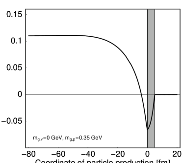
Figure 6: The difference between medium and the vacuum $0^{th}$ order energy loss for charm quarks is shown as a function of coordinate of particle production. The curves are computed by assuming running coupling given by Eq. (15), with different couplings in the medium and in the vacuum. The thickness of the medium is $L=5$ fm. The charm mass is $M=1.5$ GeV and the gluon mass is $m_{g,v}=0$ GeV ($m_{g,p}=0.35$ GeV) for the vacuum (medium) case.

Finally, in Fig. 6 we show the difference between medium and vacuum $0^{th}$ order energy loss as a function of coordinate of particle production. The figure clearly shows the transition from positive definite values (for the case when the particle is produced far outside the medium) to negative values (obtained when the particle is produced inside the medium).

4 Dependence of transition radiation on the vacuum gluon mass

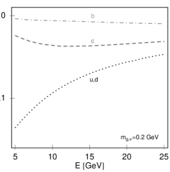
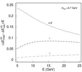
Figure 7: The difference between medium and the vacuum $0^{th}$ order fractional energy loss for light (dotted curve), charm (dashed curve) and bottom quark (dot-dashed curve) is shown as a function of the jet energy. The thickness of the medium is $L=5$ fm. The curves are computed by assuming running coupling given by Eq. (15), with different couplings in the medium and in the vacuum. Light quark mass is $M=0$ GeV, charm mass $M=1.5$ GeV, and bottom mass $M=4.5$ GeV. The gluon mass in the medium is $m_{g,p}=0.35$ GeV. Left (right) panel corresponds to the $m_{g,v}=\Lambda_{QCD}\approx 0.2$ GeV ($m_{g,v}=0.7$ GeV) case ($m_{g,v}$ is the gluon mass in the vacuum).

The analysis presented in the previous two sections is based on the assumption that $m_{g,v}=0$ in URHIC. However, this is true only in the case of the perturbative vacuum which does not take confinement into account. A phenomenological way to simulate confinement in the vacuum is to introduce an effective gluon mass $m_{g,v}\neq 0$ [21]. In this case, there are two different vacuum gluon masses that can be found in literature [22]-[24], i.e. $m_{g,v}\approx\Lambda_{QCD}$ and $m_{g,v}\approx 0.7$ GeV.

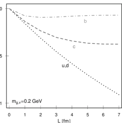
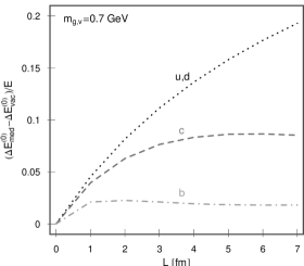
Figure 8: The difference between medium and the vacuum $0^{th}$ order fractional energy loss for light (dotted curve), charm (dashed curve) and bottom quark (dot-dashed curve) is shown as a function of the thickness of the medium. The initial jet energy is $E=15$ GeV. The curves are computed by assuming running coupling given by Eq. (15), with different couplings in the medium and in the vacuum. Light quark mass is $M=0$ GeV, charm mass $M=1.5$ GeV, and bottom mass $M=4.5$ GeV. The gluon mass in the medium is $m_{g,p}=0.35$ GeV. Left (right) panel corresponds to the $m_{g,v}=\Lambda_{QCD}\approx 0.2$ ($m_{g,v}=0.7$) GeV case ($m_{g,v}$ is the gluon mass in the vacuum).

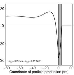
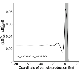
Figure 9: The difference between medium and the vacuum $0^{th}$ order energy loss for charm quarks is shown as a function of coordinate of particle production. The curves are computed by assuming running coupling given by Eq. (15), with different couplings in the medium and in the vacuum. The thickness of the medium is $L=5$ fm. The charm mass is $M=1.5$ GeV and the gluon mass in the medium is $m_{g,p}=0.35$ GeV. Left (right) panel corresponds to the $m_{g,v}=\Lambda_{QCD}\approx 0.2$ ($m_{g,v}=0.7$) GeV case ($m_{g,v}$ is the gluon mass in the vacuum).

To test how the difference between medium and vacuum $0^{th}$ order energy loss depends on the different choices of $m_{g,v}$ we first show alternatives of Figs. 3, 4 and 6 for the case of $m_{g,v}\approx\Lambda_{QCD}$ and $m_{g,v}\approx 0.7$ GeV (see Figs. 7, 8 and 9 respectively). The left panels of Figs. 7, 8 and 9 correspond to $m_{g,v}\approx\Lambda_{QCD}$ case. We see that these figures are qualitatively similar to the $m_{g,v}=0$ case, although the net effect is smaller for $m_{g,v}\approx\Lambda_{QCD}$. This result is expected, since $I_{p}^{(0)}-I_{v}^{(0)}\propto(m_{g,p}^{2}-m_{g,v}^{2})$, and $\Lambda_{QCD}>0$ GeV. On the other hand, the results shown in the right panels of Figs. 7, 8 and 9 are qualitatively different from the $m_{g,v}=0$ case. This is due to the fact that, in this case, the gluon mass in the vacuum is larger than in the medium ($m_{g,v}=0.7$ GeV), and thus we would expect that $I_{p}^{(0)}-I_{v}^{(0)}$ would always be positive definite, in agreement with these figures.

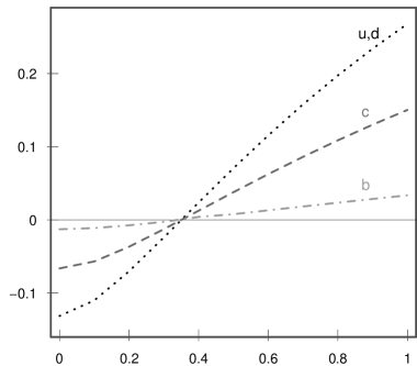
Figure 10: The difference between medium and the vacuum $0^{th}$ order energy loss is shown as a function of the gluon mass in the vacuum ($m_{g,v}$). The curves are computed by assuming running coupling given by Eq. (15), with different couplings in the medium and in the vacuum. The dotted curve corresponds to the light quarks, dashed to the charm and dot-dashed curve to the bottom quark. The initial energy of the jet is $15$ GeV, and thickness of the medium is $L=5$ fm. We take that light, charm and bottom quark masses are $M=0$, $M=1.5$ and $M=4.5$ GeV respectively.

In Fig. 10 we show the difference between medium and the vacuum $0^{th}$ order energy loss for light, charm and bottom quarks as a function of the vacuum gluon mass ($m_{g,v}$). From this figure we see that for bottom quarks the difference is negligible. For charm quarks, in the range of experimental interest ($0$ GeV $<m_{g,v}<0.7$ GeV) this difference is in the range of about $\pm 5\%$. In [25, 26] we showed that this difference has small effects on the heavy flavor experimental observables (i.e. negligible effect on bottom, and less than $\pm 0.1$ on charm $R_{AA}$). However, for the light quarks, we see that the difference between medium and the vacuum energy loss is in the range of about $\pm 15\%$, which may have a sizable effect on the pion suppression. We therefore conclude that, in order to obtain consistent predictions for pion suppression data, 1) the gluon mass in the vacuum has to be more accurately estimated and 2) the transition radiation has to be taken into account.

5 Net radiative energy loss dependence on transition radiation

In this section we will use the medium induced radiative energy loss given in [13] to study how the difference between net radiative medium ($\Delta E^{(1)}+\Delta E^{(0)}_{med}$) and the vacuum ($\Delta E^{(0)}_{vac}$) energy loss changes when the transition radiation effects are included.

5.1 Comparison between light and heavy quark medium induced radiative energy loss

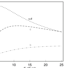
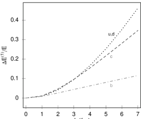
Figure 11: On the left panel the $1^{st}$ order in opacity fractional energy loss as a function of initial jet energy is shown for heavy and light quark jets. Assumed thickness of the medium is $L=5$ fm. On the right panel the $1^{st}$ order in opacity fractional energy loss for a 15 GeV jet is plotted versus the effective static thickness $L$. Plasma is characterized by $m_{g,p}=0.35$ GeV and $\lambda=1$ fm. Dotted curves corresponds to light quarks while (dashed) dot-dashed curves corresponds to charm (bottom).

For the purpose of further comparison, in this subsection, we show the $1^{st}$ order medium induced radiative energy loss for light and heavy quarks. The left panel of Fig. 11 shows fractional energy loss to $1^{st}$ order in opacity($\Delta E^{(1)}$) as a function of initial jet energy. As in the previous sections, we assume running coupling given by Eq. (15) with $m_{g}=m_{g,p}=0.35$ GeV. We take $L=5$ fm and $\lambda=1$ fm for the plasma parameters. We see that for $5$ GeV jet, the finite mass effect leads to a $50\%$ ($90\%$) reduction of the energy loss for charm (bottom) quarks. On the other hand, for a $20$ GeV jet, we see that the finite mass effect has almost no effect on charm quarks while it reduces the bottom quark energy loss by $50\%$.

On the right panel of Fig. 11 we fix the jet energy to $15$ GeV, and look at the fractional energy loss as a function of thickness of the medium. Wee see that charm and light quark energy loss dependence is similar, while bottom quark remains significantly different and close to the linear $L^{1}$ Bethe-Heitler form. This behavior is expected having in mind the left panel in Fig. 11. There we see that, for a $15$ GeV jet, the finite mass effect does not have a large influence on charm quarks, while it still has a significant influence on heavy bottom quarks.

5.2 The net radiative energy loss for light and heavy quarks in QCD medium

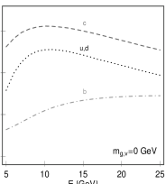
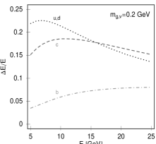
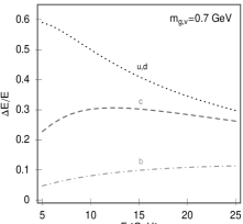
Figure 12: The net radiative fractional energy loss ($\Delta E=\Delta E^{(1)}+\Delta E^{(0)}_{med}-\Delta E^{(0)}_{vac}$) as a function of initial jet energy is shown for heavy and light quark jets. Thickness of the medium is $L=5$ fm. Left, central and right panels correspond to $m_{g,v}=0,\,0.2$ and $0.7$ GeV cases respectively. Dotted curves corresponds to light quarks, while (dashed) dot-dashed curves corresponds to charm (bottom).

In this subsection, we first concentrate how the net radiative energy loss depends on the initial jet energy for $m_{g,v}=0,\,0.2$ and $0.7$ GeV cases. Figure 12 was obtained by combining Figs. 3 and 7 with the left panel of Fig. 11. We use it to compare the net radiative energy loss results for light, charm and bottom quarks. We see that, depending on the gluon mass in the vacuum, the transition radiation may either further enhance (for $m_{g,v}>m_{g,p}$) or kill the “dead-cone” effect (for $m_{g,v}<m_{g,p}$). Additionally, we see that the transition radiation may have a significant influence on the net radiative light parton energy loss. For example, for the $m_{g,v}=0$ GeV case, the light quark energy loss is smaller than the charm quark energy loss. Additionally, in this case, the energy loss for all three types of quarks shows a weak dependence on the initial jet energy. On the other hand, in the $m_{g,v}=0.7$ GeV case, the light quark energy loss is a steeply decreasing function of initial jet energy. Additionally, this energy loss is significantly larger than both the charm and bottom quark energy losses.

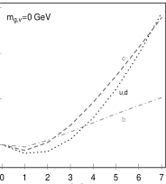
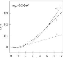
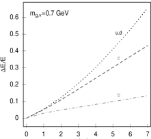
Figure 13: The net radiative fractional energy loss ($\Delta E=\Delta E^{(1)}+\Delta E^{(0)}_{med}-\Delta E^{(0)}_{vac}$) as a function of the thickness of the medium is shown for heavy and light quark jets. Initial jet energy is 15 GeV. Left, central and right panels correspond to $m_{g,v}=0,\,0.2$ and $0.7$ GeV cases respectively. Dotted curves corresponds to light quarks, while (dashed) dot-dashed curves corresponds to charm (bottom).

Figure 13 is obtained by combining Figs. 4 and 8 with the right panel of Fig. 11. We use it to compare the thickness dependence of the net radiative energy loss results for light, charm and bottom quarks. In the $m_{g,v}\lesssim\Lambda_{QCD}$ case, we see that for the light quarks, introduction of the transition radiation may lead to the cancellation of the medium induced radiative energy loss for $L\lesssim 3$ fm. This result infers that light partons may leave the medium practically unquenched if traveling the distances smaller than $3$ fm. Similar energy loss thickness dependence was already observed in [14], and the Fig. 12 may point how to solve the thickness dependence puzzle posed by [14].

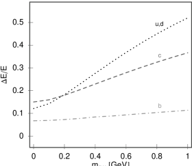
Figure 14: The net radiative fractional energy loss ($\Delta E=\Delta E^{(1)}+\Delta E^{(0)}_{med}-\Delta E^{(0)}_{vac}$) as a function of the gluon mass in the vacuum ($m_{g,v}$) is shown for heavy and light quark jets. Dotted curve corresponds to light quarks, while (dashed) dot-dashed curve corresponds to charm (bottom). Initial jet energy is $E=15$ GeV, and thickness of the medium is $L=5$ fm.

Finally in Fig. 14 we fix the jet energy and thickness of the QCD medium, and compare the $m_{g,v}$ dependence of the net radiative energy loss results for light, charm and bottom quarks. While bottom quark net radiative energy loss is independent on $m_{g,v}$, light quark shows significant dependence on the on $m_{g,v}$, as expected from Fig. 10. For example, we see that, for the $m_{g,v}<\Lambda_{QCD}$ the light quark energy loss is smaller than charm’s. On the other hand, in $m_{g,v}\approx 1$ GeV case, the difference between light and heavy quark energy loss is enhanced from $10\%$ (see 15 GeV point on Fig. 12) to approximately $40\%$.

Unfortunately, at the moment we do not know what value of $m_{g,v}$ would, most accurately, reflect confinement effects in the vacuum. However, based on Figs. 12-14 we see that the $m_{g,v}>m_{g,p}$ enhances the differences between the light and heavy quark energy loss results, and therefore would lead to a significant difference between the suppressions of light and heavy parton observables. On the other hand, $m_{g,v}<m_{g,p}$ lowers the differences between the light and heavy quark energy losses, and would correspondingly lower the differences between the suppressions of light and heavy observables. Based on the most recent experimental results [27], which suggest similar suppression results for pions (light partons observable) and single electrons (heavy quark observable), we expect that $m_{g,v}\lesssim\Lambda_{QCD}$ is the most appropriate value to approximate confinement in the vacuum.

6 Conclusions

A finite size medium, with dimensions on the order of the diameter of the collided heavy ion, is created in URHIC. Due to that, jets experience a transition from medium to the vacuum, which results in additional energy loss, called transition radiation. Since the Ter-Mikayelian was computed under the assumption of an infinite medium [10], in this paper we addressed the finite size correction to this effect.

In [10] we obtained that, due to the Ter-Mikayelian effect, the medium energy loss for charm quarks is reduced by 30 % compared to the vacuum case. We have showed that the finite size correction reduces this effect from 30% to 15%. The obtained result is intuitively unexpected, since the well known QED transition radiation calculations [9, 20] give a positive difference between the medium and the vacuum energy loss. The discrepancy between QED and QCD case results from the fact that in QED experiments a particle is produced far outside the medium, and has to cross two vacuum/medium boundaries in order to reach a detector, while in QCD experiment, the particle is produced inside the medium and crosses only one boundary. The QCD effect is therefore smaller by (approximately) the energy loss corresponding to one boundary crossing.

Previously, there was a contradiction caused by the fact that the energy loss is infinite in the vacuum and finite in the medium, leading to the infinite discontinuity between medium and the vacuum energy loss. This problem was long avoided by assuming the same zero mass for light partons in both medium and the vacuum. We here showed that this infinite discontinuity is naturally regulated by including transition radiation. To our best knowledge, the work presented here is the first consistent solution to this problem.

Further, we showed, that for $m_{g,v}\lesssim\Lambda_{QCD}$, the light parton may not loose energy when traveling distances smaller than 3 fm. This result is similar to the one experimentally observed in [14]. Consequently, one of the future goals is to understand the impact of the transition radiation to the light observable’s suppression results.

We note that our computations were done under the assumption of static medium of finite size $L$. Therefore, one of the interesting future problems is to study how these results are modified under the influence of the dynamically expanding QCD medium with continuously changing density at the edge. We expect that for a more gradual density change between the medium and vacuum, the difference between medium and vacuum $0^{th}$ order radiation is reduced.

Finally, we also note that our calculations considered only the radiative energy loss and did not take elastic energy loss into account. Recent computations by [28] show that the elastic energy loss in the QCD medium is negligible, which supports non-inclusion of the elastic energy loss into account. However, in [29] it was obtained that the elastic energy loss is significant. Consistent inclusion of the elastic energy loss into our radiative energy loss formalism is the subject of our future work.

Appendix A Gluon wave function in finite size QCD medium

In this appendix we will derive the gluon wave function in a finite size QCD medium. As already stated in Section 2, in the spinless case the wave function of the emitted gluon with momentum $k$ can be written as (see Eq. (5))

$$A_{\mu}(x)=\epsilon_{\mu}(k)\;\Phi_{g}({\mbox{x}})\;c,$$ (22)

where $\epsilon(k)=[0,2\frac{{\mbox{\scriptsize{\boldmath$\epsilon$}}}{\bf\cdot k}}{k^{+}},{\mbox{\scriptsize{\boldmath$\epsilon$}}}]$ is the transverse polarization and $c$ is the color factor of the radiated gluon. In finite size QCD medium, gluon mass (which is proportional to the temperature) becomes position dependent, and $\Phi_{g}({\mbox{x}})$ is the wave function that satisfies the Klein-Gordon equation with position dependent gluon mass $m_{g}({\mbox{x}^{+}})$.

In this section we will derive the wave function $\Phi_{g}(x)$ in the light cone coordinate system. To compute this wave function, we have to solve the fallowing equation

$$(\Box+m_{g}({\mbox{x}^{+}})^{2})\Phi_{g}(x)=0,$$ (23)

where in light cone coordinate system $\Box\equiv 4\,\partial_{{\mbox{\scriptsize x}^{+}}}\partial_{{\mbox{\scriptsize x}^{-}}}-\partial_{{\mbox{\scriptsize{\bf x}}}}^{2}$. Note that we have an extra factor of $4$ which is the consequence of the coordinate transformations. Additionally, note that Klein-Gordon equation now becomes first order in ${\mbox{x}^{+}}$ and ${\mbox{x}^{-}}$ [16, 30].

By assuming that the $\Phi_{g}({\mbox{x}})$ has the fallowing form $\Phi_{g}({\mbox{x}})=\phi_{1}({\mbox{x}^{+}})\phi_{2}({\mbox{x}^{-}})\,e^{i{\bf k\cdot x}}$, it becomes easy to show that

$$\phi_{2}({\mbox{x}^{-}})=e^{-i\frac{1}{2}k^{+}{\mbox{\scriptsize x}^{-}}}$$ (24)

where $k^{+}$ is a constant.

Klein-Gordon equation then reduces to

$$\frac{d\ln\phi_{1}({\mbox{x}^{+}})}{d{\mbox{x}^{+}}}=-i\frac{{\bf k}^{2}+m_{g}({\mbox{x}^{+}})^{2}}{2k^{+}}=-\frac{i}{2}k^{-}({\mbox{x}^{+}}),$$ (25)

where $k^{-}({\mbox{x}^{+}})\equiv\frac{{\bf k}^{2}+m_{g}({\mbox{\scriptsize x}^{+}})^{2}}{k^{+}}$. We can now easily obtain the solution for $\phi_{1}({\mbox{x}^{+}})$

$$\phi_{1}({\mbox{x}^{+}})=e^{-\frac{i}{2}\int\limits_{0}^{{\mbox{\scriptsize x}^{+}}}d\xi\,k^{-}(\xi)},$$ (26)

which, together with Eq. (24), leads to the solution of the gluon wave function in a finite size QCD medium

$$\Phi_{g}({\mbox{x}})=e^{-i\frac{1}{2}[k^{+}{\scriptsize{\mbox{x}}^{-}}+\int\limits_{0}^{{\scriptsize{\mbox{x}^{+}}}}d\xi\,k^{-}(\xi)]+i{\bf k\cdot x}}$$ (27)

This solution is valid for arbitrary gluon mass functional dependence $m_{g}({\mbox{x}^{+}})$, and is not limited to the static medium case which we consider in Section 2. In a static medium, where $m_{g}({\mbox{x}^{+}})$ is given by Eq. (7), the Eq. (27) reduces to

$$\Phi_{g}({\mbox{x}})=e^{-ik_{p}{\mbox{\scriptsize x}}}\;\theta(L-\frac{{\mbox{x}}^{+}}{2})+e^{-i(k^{-}_{p}-k^{-}_{v})L}\,e^{-ik_{v}{\mbox{\scriptsize x}}}\;\theta(\frac{{\mbox{x}}^{+}}{2}-L)$$ (28)

where

$$k_{p} = [k^{+},\frac{{\bf k}^{2}+m_{g,p}^{2}}{k^{+}},{\bf k}]\;,$$

$$k_{v} = [k^{+},\frac{{\bf k}^{2}+m_{g,v}^{2}}{k^{+}},{\bf k}]$$ (29)

is the gluon momentum in the medium and the vacuum respectively.

Appendix B Computation of $M_{rad}$ in the case when the jet is produced inside the medium

In this appendix we will compute the amplitude of the diagram $M_{rad}$ in the case when the jet is produced inside a static QCD medium of size $L$. To do that we start with the Eq. (1), i.e.

$$M^{rad}=\int d^{4}{\mbox{x}_{0}}\;J({\mbox{x}_{0}})\;d^{4}{\mbox{x}_{1}}\;\Delta_{M}({\mbox{x}_{1}}-{\mbox{x}_{0}})\;v^{\mu}({\mbox{x}_{1}})\;A_{\mu}^{\dagger}({\mbox{x}_{1}})\Phi^{\dagger}({\mbox{x}_{1}}).$$ (30)

Here $\Phi({\mbox{x}_{1}})=e^{-ip{\mbox{\scriptsize x}}}$ is the wave function of the final quark with (on-shell) momentum $p$ and $A_{\mu}({\mbox{x}_{1}})$ is the wave function of the emitted gluon. Vertex function $v^{\mu}({\mbox{x}_{1}})$ is given by $v^{\mu}({\mbox{x}_{1}})=g({\mbox{x}_{1}})(\overleftarrow{\partial}^{\mu}-\overrightarrow{\partial}^{\mu})$, where $g({\mbox{x}_{1}})$ is the running coupling constant.

After replacing Eqs. (4)-(6) in Eq.(30), we obtain (note that since x${}_{1}>$ x₀, we keep only the first term in Eq. (4))

$$M_{rad} = \int d^{4}{\mbox{x}_{0}}\;J({\mbox{x}_{0}})\;d^{4}{\mbox{x}_{1}}\;\frac{-i}{(2\pi)^{3}}\int\frac{dp^{\prime+}d^{2}{\bf p^{\prime}}}{2p^{\prime+}}\theta(({\mbox{x}}_{1}-{\mbox{x}}_{0})^{+})\;e^{-ip^{\prime}({\mbox{\scriptsize x}}_{1}-{\mbox{\scriptsize x}}_{0})}$$ (31)

$$\hskip 14.22636ptg({\mbox{x}}_{1})(\overleftarrow{\partial}^{\mu}_{{\mbox{\scriptsize x}}_{1}}-\overrightarrow{\partial}^{\mu}_{{\mbox{\scriptsize x}}_{1}})\;\epsilon_{\mu}(k)\,\Phi^{*}_{g}({\mbox{x}_{1}})\,c\;e^{ip{\mbox{\scriptsize x}}_{1}}$$

$$= \int\frac{dp^{\prime+}d^{2}{\bf p^{\prime}}}{2p^{\prime+}}\;\int d^{4}{\mbox{x}_{0}}\;J({\mbox{x}_{0}})e^{i(p+k){\mbox{\scriptsize x}}_{0}}\;\frac{-i}{(2\pi)^{3}}\;\int d^{4}{\mbox{x}_{1}}(-i)g({\mbox{x}}_{1})$$

$$\hskip 14.22636pt(p^{\prime}+p)^{\mu}\epsilon_{\mu}(k)\,e^{i(p-p^{\prime})({\mbox{\scriptsize x}}_{1}-{\mbox{\scriptsize x}}_{0})}\Phi^{*}_{g}({\mbox{x}}_{1}-{\mbox{x}}_{0})\theta(({\mbox{x}}_{1}-{\mbox{x}}_{0})^{+})\;c.$$

In the static medium we can replace $\Phi_{g}({\mbox{x}})$ by Eq. (28), and the Eq. (31) reduces to (note ${\mbox{x}}={\mbox{x}}_{1}-{\mbox{x}}_{0}$)

$$M_{rad} = \int\frac{dp^{\prime+}d^{2}{\bf p^{\prime}}}{2p^{\prime+}}\;J(p+k)\;(2p^{\prime}\cdot\epsilon)$$ (32)

$$\hskip 14.22636pt\{\frac{-i}{(2\pi)^{3}}\;\int d^{4}{\mbox{x}}\;(-i)g_{p}\;e^{i(p+k_{p}-p^{\prime}){\mbox{\scriptsize x}}}\;\theta({\mbox{x}}^{+})\theta(L-\frac{{\mbox{x}}^{+}}{2})$$

$$\hskip 14.22636pt\;+\;e^{i(k^{-}_{p}-k^{-}_{v})L}\,\frac{-i}{(2\pi)^{3}}\;\int d^{4}{\mbox{x}}\;(-i)g_{v}\;e^{i(p+k_{v}-p^{\prime}){\mbox{\scriptsize x}}}\;\theta(\frac{{\mbox{x}}^{+}}{2}-L)\}\;c\;,$$

where we used $J(p+k)=\int d^{4}{\mbox{x}_{0}}\;J({\mbox{x}_{0}})e^{i(p+k){\mbox{\scriptsize x}}_{0}}$.

We will first compute $I_{1}=\frac{-i}{(2\pi)^{3}}\;\int d^{4}{\mbox{x}}\;(-i)g_{p}\;e^{i(p+k_{p}-p^{\prime}){\mbox{\scriptsize x}}}\;\theta({\mbox{x}}^{+})\theta(L-\frac{{\mbox{x}}^{+}}{2})$. Note that in the light cone gauge $d^{4}{\mbox{x}}=1/2\,d{\mbox{x}}^{+}d{\mbox{x}}^{-}d{\bf x}$, leading to

$$I_{1} = \frac{-g_{p}}{(2\pi)^{3}}\;\int 1/2\,d{\mbox{x}}^{+}d{\mbox{x}}^{-}d{\bf x}\;e^{\frac{i}{2}(p+k-p^{\prime})^{+}{\mbox{\scriptsize x}}^{-}}\;e^{\frac{i}{2}(p+k_{p}-p^{\prime})^{-}{\mbox{\scriptsize x}}^{+}}e^{-i{\bf(p+k-p^{\prime})\cdot x}}\;\theta({\mbox{x}}^{+})\theta(L-\frac{{\mbox{x}}^{+}}{2})$$ (33)

$$= -g_{p}\;\delta(p^{+}+k^{+}-p^{\prime+})\delta({\bf p+k-p^{\prime}})\int_{0}^{2L}d{\mbox{x}}^{+}\;e^{\frac{i}{2}(p+k_{p}-p^{\prime})^{-}{\mbox{\scriptsize x}}^{+}}$$

$$= -2ig_{p}\;\delta(p^{+}+k^{+}-p^{\prime+})\delta({\bf p+k-p^{\prime}})\frac{1-e^{i(p+k_{p}-p^{\prime})^{-}L}}{(p+k_{p}-p^{\prime})^{-}}$$

Without loss of generality, we can take for the initial quark the plane wave state in the ${\bf x}$-plane and set ${\bf p^{\prime}}=0$. Then ${\bf p}=-{\bf k}$, and $(p+k_{p}-p^{\prime})^{-}=\chi_{p}$, where $\chi_{p}$ is given by Eq. (9). By using this, the Eq. (33) finally reduces to

$$I_{1}=-2ig_{p}\;\delta(p^{+}+k^{+}-p^{\prime+})\delta({\bf p+k-p^{\prime}})\frac{1-e^{i\chi_{p}L}}{\chi_{p}}$$ (34)

In the same way $I_{2}=e^{i(k^{-}_{p}-k^{-}_{v})L}\,\frac{-i}{(2\pi)^{3}}\;\int d^{4}{\mbox{x}}\;(-i)g_{v}\;e^{i(p+k_{v}-p^{\prime}){\mbox{\scriptsize x}}}\;\theta(\frac{{\mbox{x}}^{+}}{2}-L)$ reduces to

$$I_{2} = -2ig_{p}\;e^{-i(k^{-}_{p}-k^{-}_{v})L}\delta(p^{+}+k^{+}-p^{\prime+})\delta({\bf p+k-p^{\prime}})\frac{e^{i\chi_{v}L}}{\chi_{v}}$$ (35)

$$= -2ig_{p}\;\delta(p^{+}+k^{+}-p^{\prime+})\delta({\bf p+k-p^{\prime}})\frac{e^{i\chi_{p}L}}{\chi_{v}}$$

After we plug in the Eqs. (34) and (35) into Eq. (31) and use $(p^{\prime}\cdot\epsilon)=\frac{{\mbox{\scriptsize{\boldmath$\epsilon$}}}{\bf\cdot k}}{x}$ ($x\equiv\frac{k^{+}}{p^{\prime+}}$), the $M_{rad}$ reduces to

$$M_{rad} = -2i\int{dp^{\prime+}d^{2}{\bf p^{\prime}}}\;J(p+k)\;(p^{\prime}\cdot\epsilon)\;\delta(p^{+}+k^{+}-p^{\prime+})\;\delta({\bf p+k-p^{\prime}})$$ (36)

$$\;(\frac{g_{p}}{p^{\prime+}}\frac{1-e^{i\chi_{p}L}}{\chi_{p}}+\frac{g_{v}}{p^{\prime+}}\frac{e^{i\chi_{p}L}}{\chi_{v}})\;c$$

$$= -2i\,J(p+k)\frac{{\mbox{\boldmath$\epsilon$}}{\bf\cdot k}}{x}\left[\frac{g_{p}}{p^{\prime+}}\frac{1-e^{i\chi_{p}L}}{\chi_{p}}+\frac{g_{v}}{p^{\prime+}}\frac{e^{i\chi_{p}L}}{\chi_{v}}\right]c\;,$$

which is the Eq. (8) given in section 2.

Appendix C Computation of $M_{rad}$ in the case when the jet is produced outside the medium

In this appendix we will compute the Eq. (31) in the case when the jet is produced at the distance $l_{0}$ from the medium, i.e. at $\mbox{x}_{0}^{+}=-2l_{0}<0$. Then, for $\mbox{x}=\mbox{x}_{1}-\mbox{x}_{0}$, (where $\mbox{x}_{1}$ is the gluon production point), $m_{g}({\mbox{x}^{+}})$ can be written as

$$m_{g}({\mbox{x}^{+}})=m_{g,v}\;\theta({\mbox{x}^{+}})\theta(l_{0}-\frac{{\mbox{x}^{+}}}{2})+m_{g,p}\;\theta(\frac{{\mbox{x}^{+}}}{2}-l_{0})\theta(l_{0}+L-\frac{{\mbox{x}^{+}}}{2})+m_{g,v}\;\theta(\frac{{\mbox{x}^{+}}}{2}-(L+l_{0}))$$ (37)

By using Eq. (37), $\Phi_{g}({\mbox{x}})$ (see Eq. (27)) reduces to

$$\Phi_{g}({\mbox{x}}) = e^{-ik_{v}{\mbox{\scriptsize x}}}\;\theta({\mbox{x}^{+}})\theta(l_{0}-\frac{{\mbox{x}^{+}}}{2})+e^{-i(k^{-}_{v}-k^{-}_{p})l_{0}}e^{-ik_{p}{\mbox{\scriptsize x}}}\;\theta(\frac{{\mbox{x}^{+}}}{2}-l_{0})\theta(l_{0}+L-\frac{{\mbox{x}^{+}}}{2})$$ (38)

$$\hskip 110.96556pt+e^{-i(k^{-}_{p}-k^{-}_{v})L}e^{-ik_{v}{\mbox{\scriptsize x}}}\;\theta(\frac{{\mbox{x}^{+}}}{2}-(L+l_{0}))$$

With the use of Eq. (38), the Eq. (31) reduces to

$$M_{rad} = \int\frac{dp^{\prime+}d^{2}{\bf p^{\prime}}}{2p^{\prime+}}\;J(p+k)\;(2p^{\prime}\cdot\epsilon)$$ (39)

$$\hskip 14.22636pt\{\frac{-i}{(2\pi)^{3}}\;\int d^{4}{\mbox{x}}\;(-i)g_{v}\;e^{i(p+k_{v}-p^{\prime}){\mbox{\scriptsize x}}}\;\theta({\mbox{x}}^{+})\theta(l_{0}-\frac{{\mbox{x}}^{+}}{2})$$

$$\hskip 14.22636pt\;+\;e^{i(k^{-}_{v}-k^{-}_{p})l_{0}}\,\frac{-i}{(2\pi)^{3}}\;\int d^{4}{\mbox{x}}\;(-i)g_{p}\;e^{i(p+k_{p}-p^{\prime}){\mbox{\scriptsize x}}}\;\theta(\frac{{\mbox{x}^{+}}}{2}-l_{0})\theta(l_{0}+L-\frac{{\mbox{x}^{+}}}{2})$$

$$\hskip 14.22636pt\;+\;e^{i(k^{-}_{p}-k^{-}_{v})L}\,\frac{-i}{(2\pi)^{3}}\;\int d^{4}{\mbox{x}}\;(-i)g_{v}\;e^{i(p+k_{v}-p^{\prime}){\mbox{\scriptsize x}}}\;\theta(\frac{{\mbox{x}^{+}}}{2}-(L+l_{0}))\}\;c\;.$$

By applying the same procedure as in Appendix B, $M_{rad}$ finally reduces to

$$M_{rad} = -2i\int{dp^{\prime+}d^{2}{\bf p^{\prime}}}\;J(p+k)\;(p^{\prime}\cdot\epsilon)\;\delta(p^{+}+k^{+}-p^{\prime+})\;\delta({\bf p+k-p^{\prime}})$$ (40)

$$\hskip 28.45274pt\;(\frac{g_{v}}{p^{\prime+}}\frac{1-e^{i\chi_{v}l_{0}}}{\chi_{v}}+\frac{g_{p}}{p^{\prime+}}e^{i(k^{-}_{v}-k^{-}_{p})l_{0}}\frac{e^{i\chi_{p}l_{0}}-e^{i\chi_{p}(L+l_{0})}}{\chi_{p}}$$

$$\hskip 101.00737pt+\frac{g_{v}}{p^{\prime+}}\;e^{i(k^{-}_{p}-k^{-}_{v})L}\frac{e^{i\chi_{v}(L+l_{0})}}{\chi_{v}})\;c$$

$$= -2i\int{dp^{\prime+}d^{2}{\bf p^{\prime}}}\;J(p+k)\;(p^{\prime}\cdot\epsilon)\;\delta(p^{+}+k^{+}-p^{\prime+})\;\delta({\bf p+k-p^{\prime}})$$

$$\hskip 28.45274pt\;(\frac{g_{v}}{p^{\prime+}}\frac{1-e^{i\chi_{v}l_{0}}}{\chi_{v}}+\frac{g_{p}}{p^{\prime+}}\frac{e^{i\chi_{v}l_{0}}-e^{i(\chi_{p}L+\chi_{v}l_{0})}}{\chi_{p}}+\frac{g_{v}}{p^{\prime+}}\;\frac{e^{i(\chi_{p}L+\chi_{v}l_{0})}}{\chi_{v}})\;c$$

$$= -2i\,J(p+k)\frac{{\mbox{\boldmath$\epsilon$}}{\bf\cdot k}}{x}\frac{1}{p^{\prime+}}\left[\frac{g_{v}}{\chi_{v}}-(\frac{g_{v}}{\chi_{v}}-\frac{g_{p}}{\chi_{p}})e^{i\chi_{v}l_{0}}(1-e^{i\chi_{p}L})\right]$$

which is the Eq. (19) given in section 3.

References

- [1] M. Gyulassy, Lect. Notes Phys. 583, 37 (2002).
- [2] M. Gyulassy and M. Plumer, Nucl. Phys. A 527, 641 (1991).
- [3] M. Gyulassy, M. Plumer, M. Thoma and X. N. Wang, Nucl. Phys. A 538, 37C (1992); X. N. Wang and M. Gyulassy, Phys. Rev. Lett. 68, 1480 (1992).
- [4] M. Guylassy, I. Vitev, X. N. Wang and B. W. Zhang, Quark Gluon Plasma 3, editors: R.C. Hwa and X.N. Wang, World Scientific, Singapore, 123 (2003) (nucl-th/0302077).
- [5] R. Baier, Yu. L. Dokshitzer, A. H. Mueller and D. Schiff, Phys. Rev. C 58, 1706 (1998).
- [6] R. Baier, D. Schiff, B. G. Zakharov, Ann. Rev. Nucl. Paer. Sci. 50, 37 (2000).
- [7] A. Kovner and U. A. Wiedemann, Quark Gluon Plasma 3, editors: R.C. Hwa and X.N. Wang, World Scientific, Singapore, 192 (2003) (hep-ph/0304151).
- [8] M. L. Ter-Mikayelian, Dokl. Akad. Nauk SSSR 94, 1033 (1954).
- [9] M. L. Ter-Mikayelian, High-Energy Electromagnetic Processes in Condensed Media, John Wiley sons, New York (1972).
- [10] M. Djordjevic and M. Gyulassy, Phys. Rev. C 68, 034914 (2003).
- [11] M. Djordjevic and M. Gyulassy, Phys. Lett. B 560, 37 (2003).
- [12] R. D. Field, Applications of Perturbative QCD, Perseus Books, Cambridge, Massachusetts (1995).
- [13] M. Djordjevic and M. Gyulassy, Nucl. Phys. A 733, 265 (2004).
- [14] S. Mioduszewski for the PHENIX Collaboration, talk given at DNP 2004 Fall Meeting, Chicago, Illinois (2004); B. Cole for the PHENIX Collaboration, talk given at Hard Probes 2004 Conference, Lisabon, Portugal (2004).
- [15] B. G. Zakharov, JETP Lett. 76, 201 (2002).
- [16] J. B. Kogut, D. E. Soper, Phys. Rev. D 1, 2901 (1970).
- [17] M. Gyulassy, P. Levai and I. Vitev, Nucl. Phys. B 594, 371 (2001).
- [18] Y. L. Dokshitzer, V. A. Khoze and S. I. Troian, Phys. Rev. D 53, 89 (1996).
- [19] Y. L. Dokshitzer and D. E. Kharzeev, Phys. Lett. B 519, 199 (2001).
- [20] J. D. Jackson, Classical Electrodynamics, John Wiley Sons, 3rd edition (1998).
- [21] N. N. Nikolaev and B. G. Zakharov, Phys. Lett. B 327, 149 (1994).
- [22] G. Sterman and P. Stoler, Ann. Rev. Nucl. Part. Sci. 47 193 (1997).
- [23] C. Alexandrou, Ph. de Forcrand and E. Follana, Phys. Rev. D 65, 114508 (2002); K. Langfeld, H. Reinhardt and J. Gattnar, Nucl. Phys. B 621, 131 (2002).
- [24] J. H. Field, Phys. Rev. D 66, 013013 (2002).
- [25] M. Djordjevic, M. Gyulassy and S. Wicks, Eur. Phys. J. C 43, 135 (2005).
- [26] M. Djordjevic, M. Gyulassy and S. Wicks, Phys. Rev. Lett. 94, 112301 (2005).
- [27] Y. Akiba [the PHENIX Collaboration], arXiv:nucl-ex/0510008. S. A. Butsyk, arXiv:nucl-ex/0510010. X. Dong, arXiv:nucl-ex/0509038.
- [28] S. Peigne, P. B. Gossiaux, T. Gousset, hep-ph/0509185.
- [29] M. G. Mustafa, Phys. Rev. C 72, 014905 (2005).
- [30] J. D. Bjorken, J. B. Kogut and D. E. Soper, Phys. Rev. D 3, 1382 (1971).