Strangeness dynamics in heavy-ion collisions:
the $K/\pi$ ratios and the lifetime of a fireball

Abstract

We propose a non-equilibrium, hadronic kinetic model for describing the relative abundance of strange particles in ultra-relativistic heavy-ion collisions. The energy dependence of the multiplicity ratios of charged kaons and lambdas to pions are studied in detail. The pronounced peak in $\langle K^{+}\rangle/\langle\pi^{+}\rangle$ is conjectured to be due to the decreasing lifetime of a fireball with an increase in beam energy above 30 $A$GeV. Such a behaviour may be the consequence of a stronger stopping at lower beam energies. We study the dependence of the multiplicity ratios on energy and baryon density of the fireball and its total lifetime.

I Strangeness production in nuclear collisions

The excitation functions of multiplicity ratios of kaons to pions are among the most intriguing results of the energy scan at CERN’s Super-Proton-Synchrotron alt20 ; ktpdata . The sharp peak of the ratio $\langle K^{+}\rangle/\langle\pi^{+}\rangle$ for collisions at beam energy of 30 $A$GeV—dubbed “the horn”—is barely reproduced by any theoretical calculation. The statistical model expects a maximum in this region, which is due to the transition from baryon-dominated to meson-dominated matter Cleymans:2004hj . That maximum is, however, much broader than the observed sharp peak. Transport models UrQMD and HSD UrQMDHSD overpredict $\pi^{+}$ production and predict a very modest bump which is lower than the measured horn and lies at lower beam energy. The BUU model of moselBUU shows no peaky structure at all. Three-fluid hydrodynamic model toneev reproduces the $K^{+}$ and pion yields but overpredicts a multiplicity of $K^{-}$. Recently, a kinetic model which assumes a phase-transition to the deconfined phase has been proposed and was successfull in reproducing the data jane .

The data can be interpreted in the framework of the Statistical Model of the Early Stage (SMES) smes . In this model it is assumed that the primordial particle production follows the prescription of statistical equilibrium. The increase of the $\langle K^{+}\rangle/\langle\pi^{+}\rangle$ ratio at low collision energies is a consequence of an enhanced strangeness content due to a larger energy deposit. The sharp decrease of the ratio above the beam energy of 30 $A$GeV is connected with a first order phase transition between hadronic and deconfined phases. The decreasing part of the excitation function corresponds to the mixture of the two phases, while the flat dependence at high energies is realized in the deconfined phase. In framework of SMES, this observation is taken as partial evidence for deconfinement in the nuclear collisions at threshold energy $\sqrt{s_{NN}}\approx 7.6\,\mbox{GeV}$ ($E_{\rm beam}=30\,A\mbox{GeV}$).

At this point we would like to pose two questions which provide the motivation for our study. Firstly, is the assumption of chemically equilibrated primordial production justified? This is not obvious at all. Analysis within a statistical hadronization model shows that the limited volume in proton-proton collisions causes suppression of strangeness once canonical statistics is used. On the other hand, a large volume allows for the use of grand-canonical statistics and leads to enhanced strangeness content redlich . But how could the incident nucleons be influenced by volume effects in the very moment of their first interactions? Secondly, one cannot claim evidence of deconfinement unless all hadronic scenarios have been safely ruled out. We shall not touch here the question of early thermalization at the SPS. In this paper we investigate if all hadronic (non-equilibrium) models are safely excluded after comparison with the data.

We propose a model in which strangeness is produced dynamically in reactions involving the constituent hadrons of the fireball. Two aspects are crucial for the final total amount of produced strangeness: the energy density and the time. The energy density is reflected in the temperature and an increase of temperature enhances the strangeness production rate. On the other hand, at least for a non-expanding system, if the initial amount of strangeness is below the equilibrium value, it will certainly increase with time until it saturates. Thus a longer lifetime also means higher strangeness content. Based on these considerations we speculate that the initial increase of the $\langle K^{+}\rangle/\langle\pi^{+}\rangle$ excitation function is due to increasing energy density. Can the following sharp decrease of the excitation function be due to decreasing total lifetime of the fireball with increasing collision energy?

The assumption of decreasing total lifetime is crucial. Sometimes, just the opposite is expected. Due to a higher initial energy density at higher beam energies it would take a longer time for the fireball to cool down to the critical density when it breaks up. Also, a larger multiplicity at higher energies assumes a larger volume at freeze-out and thus requires longer lifetime. These arguments, however, neglect nuclear stopping and the need to build up longitudinal expansion. For example, the proper time between impact and the freeze-out comes out more or less independent of the beam energy in the transport code HSD casspriv . Indeed, it seems reasonable to expect that stopping power or an ability for slowing down incident baryons is stronger at lower energies than at higher energies. Then, a large part of the longitudinal expansion flow must be built up by the pressure at lower collision energies, and this takes time. At higher collision energies, fast expansion may be present from the very beginning and the fireball would reach a breakup stage earlier. We should stress that there is no direct measurement of stopping power as it results in rapidity distributions just after the primordial nucleon-nucleon collisions. Measured rapidity spectra reflect distributions at freeze-out, i.e., after the possibly accelerated longitudinal expansion. We know that there is some stopping at RHIC since the net baryon spectra are peaked at a rapidity lower than $y_{\rm beam}$ brahms-stopping . We also know that stopping is incomplete even down at SIS energies (few hundreds $A$MeV) as it was demonstrated by isospin tracing in collisions of ${}^{96}_{44}\mbox{Ru}$ and ${}^{96}_{40}\mbox{Zr}$ fopi . It is natural to expect that the relevant evolution scenario at AGS and SPS energies will be somewhere between full stopping and re-expansion (Landau scenario) and boost-invariant non-accelerated longitudinal expansion (Bjorken expansion).

In our model we shall adopt an ansatz for the time dependence of energy density and baryon density of the fireball. Our calculation is not based on any transport/cascade models or hydrodynamic simulation. Therefore we do not directly connect to details of microscopic structure of the matter or the equation of state. We gain, however, the freedom to construct as many different evolution scenarios as we wish, and we shall use this freedom to explore various scenarios, their impact on data, and identify those which are allowed by data. In particular, we shall focus on the dependence of total production of strange particles on the lifetime of the system. We present results for multiplicity ratios $\langle K^{+}\rangle/\langle\pi^{+}\rangle$, $\langle K^{-}\rangle/\langle\pi^{-}\rangle$, and $\langle\Lambda\rangle/\langle\pi\rangle$. It will turn out that a non-equilibrium hadronic scenario cannot be excluded by this set of data.

II The model

We shall only calculate ratios of yields and not the yields themselves. Therefore, it will be sufficient to know average densities of individual species if we assume that they come from the same volume. (Feed-down from resonance decays is also necessary, but we defer its discussion for later.) Applying later this approach to kaons ($K^{+}$ and $K^{0}$), we implicitly assume that kaons do not decouple from the system until the overall freeze-out. This is in line with a class of hydro-chemical models knoll1 ; knoll2 ; broko . This assumption will be supported by the analysis of the kaon scattering rate and the mean free path in Section II.3.

The evolution of kaon density in proper time is described by the master equation which can be derived from

$$\frac{d\rho_{K}}{d\tau}=\frac{d}{d\tau}\frac{N_{K}}{V}=\rho_{K}\,\left(-\frac{1}{V}\,\frac{dV}{d\tau}\right)+\frac{1}{V}\,\frac{dN_{K}}{d\tau}\,.$$ (1)

The first term on the right-hand-side is due to the change of a fireball volume and includes the expansion rate. The expansion rate is the change of the density of any conserved charge due to expansion. For example the relation

$$-\frac{1}{V}\frac{dV}{d\tau}=\frac{1}{\rho_{B}}\,\frac{d\rho_{B}}{d\tau}$$ (2)

holds for the baryon number. The second term on the right-hand-side of eq. (1) stands for the change of a kaon number due to production or annihilation reactions. It can be divided into gain term and loss term

$$\frac{dN_{K}}{d\tau} = V\big{(}\mathcal{R}_{\rm gain}-\mathcal{R}_{\rm loss}\big{)}$$

$$\mathcal{R}_{\rm gain} = \sum_{i\,j\,X}\left\langle v_{ij}\sigma_{ij}^{KX}\right\rangle\,\frac{\rho_{i}\,\rho_{j}}{1+\delta_{ij}}+\rho_{K^{*}}\,\Gamma_{K*}$$

$$\mathcal{R}_{\rm loss} = \sum_{i\,X}\left\langle v_{Ki}\sigma_{Ki}^{X}\right\rangle\,\frac{\rho_{K}\,\rho_{i}}{1+\delta_{Ki}}\,.$$ (3)

Terms in angular brackets are the cross-sections for reactions $ij\to KX$ or $Ki\to X$ which are multiplied by relative velocities of incoming particles and averaged over distribution of relative velocities. Here, $i$ and $j$ denote any single species with densities $\rho_{i}$ and $\rho_{j}$, and $X$ stands for any number of any species. The sums run, in principle, over all possible reaction channels. In practice they are truncated after the most significant contributions have been included.

Using eq. (3), the master equation for kaon density evolution can be written

$$\frac{d\rho_{K}}{d\tau}=\rho_{K}\,\left(-\frac{1}{V}\,\frac{dV}{d\tau}\right)+\mathcal{R}_{\rm gain}-\mathcal{R}_{\rm loss}$$ (4)

In our study we shall evolve densities of $K^{+}$, $K^{0}$, $K^{*+}$, and $K^{*0}$ according to this equation. We shall explain how densities for other strange species are obtained in Section II.2.

II.1 Expansion dynamics

In order to calculate the production and annihilation rates we need the densities of interacting species and distribution of relative velocities. These follow from the energy density $\varepsilon$ and the densities of conserved charges, baryon number $\rho_{B}$ and the third component of isospin $\rho_{3}$, which is also related to the electric charge. We shall assume thermal equilibrium and use $\varepsilon,\,\rho_{B}$ and $\rho_{3}$ to calculate temperature. The temperature determines the distribution of relative velocities. From the time-dependence of $\rho_{B}$ we shall obtain the expansion rate.

We want to be able to explore a variety of possible expansion scenarios. We shall tune the amount of stopping which is directly connected with the time-derivative of the density at the beginning. Less stopping leads to larger negative time-derivative of $\rho_{B}$ because of the initial stage expansion. Explored scenarios can also differ in the initial acceleration due to inner pressure. To include these two effects in a simplest possible way, we use quadratic dependence as an Ansatz for the initial time-dependence of the energy density

$$\varepsilon(\tau)=\varepsilon_{0}(1-a\tau-b\tau^{2})$$ (5a)

with $$\varepsilon_{0} a b$$, , and being tunable parameters. In correspondence to this we use for the initial time dependence of conserved charge densities

$$\rho_{i}(\tau)=\rho_{i0}(1-a\tau-b\tau^{2})^{\delta}$$ (5b)

where the index $i$ stands for any of the two conserved charges. The power $\delta$ is used here as the simplest way of representing the equation of state. For example, in case of non-interacting freely streaming gas no work is performed by pressure and the energy density follows the same time-dependence as baryon density, $\delta=1$. On the other hand, maximum pressure is present in a massless gas, in which $\rho_{B}\propto\varepsilon^{3/4}$, $\delta=3/4$. We shall write

$$\delta=\frac{1}{1+\kappa}\,,\qquad 0\leq\kappa\leq\frac{1}{3}\,.$$ (6)

The dependence of Hanbury-Brown/Twiss correlation radii on the transverse momentum of a pair indicates that at late times the fireball expansion follows a power-law in time

$$\varepsilon(\tau) = \frac{\varepsilon_{0}^{\prime}}{(\tau-\tau_{0})^{\alpha/\delta}},$$ (7a)

$$\rho_{i}(\tau) = \frac{\rho_{i0}^{\prime}}{(\tau-\tau_{0})^{\alpha}}.$$ (7b)

The power $\alpha$ is a model parameter. The value of $\alpha=1$ corresponds to a one-dimensional boost-invariant expansion (Bjorken scenario). Due to transverse flow, $\alpha$ acquires values larger than 1. The parameter $\tau_{0}$ allows for a shift of the power-law prescription (7) to later times and leaves thus time for acceleration.

Ansatz for initial times (5) is matched with the prescription for late times (7) at some moment $\tau_{s}$. We require continuous time dependence together with its first time derivative. In summary, the time dependence is given by

$$\varepsilon(\tau) = \begin{cases}\varepsilon_{0}(1-a\tau-b\tau^{2})&:\quad\tau<\tau_{s}\\ \frac{\varepsilon_{0}^{\prime}}{(\tau-\tau_{0})^{\alpha/\delta}}&:\quad\tau\geq\tau_{s}\end{cases},$$ (8a)

$$\rho_{i}(\tau) = \begin{cases}\rho_{i0}(1-a\tau-b\tau^{2})^{\delta}&:\quad\tau<\tau_{s}\\ \frac{\rho_{i0}^{\prime}}{(\tau-\tau_{0})^{\alpha}}&:\quad\tau\geq\tau_{s}\end{cases}.$$ (8b)

For the energy density we have parameters $\varepsilon_{0}$, $a$, $b$, $\varepsilon_{0}^{\prime}$, $\tau_{0}$, $\tau_{s}$, $\alpha$, and $\delta$, out of which two are constrained by matching conditions at $\tau_{s}$. In addition to this, for both baryon and $I_{3}$ density there are $\rho_{i0}$ and $\rho_{i0}^{\prime}$ which are connected by the requirement of continuity as well.

The parameters which appear in eqs. (8) are not directly related to measurements and/or one may not have good feeling for what their reasonable values should be. Therefore, for practical application, we shall specify the time evolution in terms of the following quantities:
$\varepsilon_{0}$ initial energy density, $\tau_{T}$ total lifetime of the fireball until chemical freeze-out after which no change of number of strange hadrons occurs; this time must be bigger than $\tau_{s}$, $\varepsilon_{f}$ final energy density, $\rho_{Bf}$ final baryon density, $\rho_{3f}$ final density of the third component of isospin $I_{3}$, $\tau_{0}$ reference time for the power-law dependence in the late stage of evolution; in principle, it is the time $(\tau_{T}-\tau_{0})$ which would appear in expansion velocity gradients at freeze-out; $(\tau-\tau_{0})$ is also the time measured by longitudinal HBT radius, $\alpha$ exponent of the late-stage power-law expansion; $\alpha=1$ corresponds to one-dimensional scaling expansion, $\alpha=3$ means three-dimensional Hubble flow $\delta$ exponent characterizing the underlying equation of state, ${\cal R}_{\rm max}$ the maximum expansion rate, which is equal to the negative of maximum decrease rate of baryon density $(-1/\rho_{B})\,(d\rho_{B}/d\tau)$ (${\cal R}_{\rm max}$ is always positive number); the maximum rate is achieved at $\tau_{s}$.
We list in Appendix A relations between these physical parameters and those of parameterizations (8).

The main parameters, which influence on the final strangeness yields we shall study below, are the initial energy density $\varepsilon_{0}$ and the total lifetime of the fireball $\tau_{T}$. The final state parameters $\varepsilon_{f}$, $\rho_{Bf}$, $\rho_{3f}$ will be calculated from the thorough analyses of various particle ratios in the chemical freeze-out model becatt . Parameters $\tau_{0}$ and $\alpha$ will be chosen to agree with femtoscopy analyses lpsw . We shall choose a value for $\delta$ and fix it and $R_{\rm max}$ can be varied only in very limited range and has little influence on the results.

The expansion rate needed in equation (4) is obtained by taking time-derivative of eq. (8b). Using eq. (2) we have

$$-\frac{1}{V}\,\frac{dV}{d\tau}=\begin{cases}-\frac{\delta(a+2b\tau)}{1-a\tau-b\tau^{2}}&:\quad\tau<\tau_{s}\\ -\frac{\alpha}{\tau-\tau_{0}}&:\quad\tau\geq\tau_{s}\end{cases}\,.$$ (9)

   

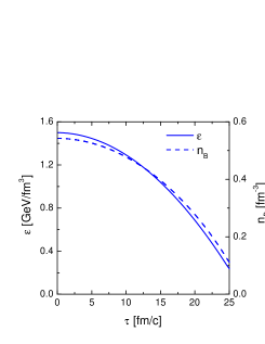
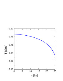
Figure 1: Left panel: the energy density (left scale) and the baryon density (right scale) as a function of time for a scenario that reproduces the data from 30 $A$GeV collisions. Right panel: the corresponding time dependence of the temperature.

For illustration we plot in Fig. 1 the time dependence of the energy density and baryon density and the temperature. The curves correspond to the scenario which reproduces experimental data on $\langle K^{+}\rangle/\langle\pi^{+}\rangle$, $\langle K^{-}\rangle/\langle\pi^{-}\rangle$, and $\langle\Lambda\rangle/\langle\pi\rangle$ ratios for 30 $A$GeV collisions as it is shown in Fig. 11 with parameters listed in Tables 1 and 3. Time evolutions in other scenarios are qualitatively very similar to the one presented here. It turns out that the shape of the curves is almost specified by the initial and final energy density and the lifetime. In fact, most of the time the fireball spends in the regime of accelerated expansion while the power law is realized only towards the end. This is driven by the requirement of a rather low initial energy density. Since the final density is fixed by the data, a longer power law tail leads readily to very high initial energy densities. We emphasize that the proposed evolution does not contradict to observations related to the freeze-out stage of a fireball expansion reconstructed via single-particle spectra and femtoscopy.

II.2 Chemical composition and reactions

For the sake of averaging over relative velocities, we shall assume that the momenta are distributed according to Boltzmann distribution

$$n_{i}(p)\propto\exp\left(-\frac{\sqrt{m_{i}^{2}+p^{2}}}{T}\right)\,.$$ (10)

Thus we make an assumption of thermal equilibrium, though chemically the system will be treated as non-equilibrated. The averaged cross section is then obtained as koform

$$\langle v_{ij}\sigma_{ij}^{X}\rangle=\\ \frac{\int_{\sqrt{s_{0}}}^{\infty}dx\,\sigma_{ij}^{X}(x)\,K_{1}\left(\frac{x}{T}\right)\,\left[x^{2}-(m_{i}+m_{j})^{2}\right]\left[x^{2}-(m_{i}-m_{j})^{2}\right]}{4\,m_{i}^{2}\,m_{j}^{2}\,T\,K_{2}(m_{i}/T)\,K_{2}(m_{j}/T)}$$ (11)

where $K_{i}$’s are the modified Bessel functions and $\sqrt{s_{0}}=\max(m_{i}+m_{j},\,\sum_{\rm final}m_{a})$ is the reaction threshold.

The following reaction channels producing kaons were taken into account

(20)

In order to keep the detailed balance we also included the inverse reactions for all channels with two particles in final state. Those processes with three and more final state particles are rather suppressed due to high thresholds and smaller phase space. By the same reason we neglect strange antibaryons. The error we thus introduce is small, because the matter is rather baryon-dominated in the investigated energy domain. The ratio $\bar{\Lambda}/\Lambda$ is about 10% at the highest SPS energy, so our discrepancy will be at most of this order. This is acceptable for a schematic model like the present one.

Only production of $K=(K^{+},K0)$ and $K^{*}=(K^{*+},K^{*0})$ mesons will be calculated from master equation (4) by including the above reaction channels. All the explicitly calculated species contain strange antiquark. They are produced being accompanied by strange and multistrange baryons, and $\bar{K}$ and $\bar{K}^{*}$ mesons containing a strange quark. In principle, we could trace density evolutions of those species kinetically. In practice, however, the reactions which do not create strange quarks but rather rearrange them in different hadrons are very quick. Therefore with a good approximation we can assume that all species containing strange quarks are in relative chemical equilibrium. In our calculations we include $K^{-}$, $\bar{K}^{0}$, $K^{*-}$, $\bar{K}^{*0}$, $\Lambda$, $\Sigma$, $\Lambda(1405)$, $\Lambda(1520)$, $\Sigma(1385)$, $\Xi$, and $\Omega$.

For the non-strange sector we assume that all species are chemically equilibrated. We included into calculations all non-strange mesons with masses below 1.5 GeV and baryons up to 2 GeV.

Since we follow evolution of every isospin state separately, we do not use isospin-averaged parameterizations for the cross sections. Appropriate cross section for every isospin channel is used instead. We list the used parameterizations in Appendix B.

For the calculation of densities of individual species and the evaluation of the average in eq. (11) we thus need the temperature $T$, and chemical potentials $\mu_{B}$ and $\mu_{3}$ connected with the baryon number and the third component of isospin, respectively. We also need phase-space occupation factors for kaons $\gamma_{K^{+}}$, $\gamma_{K^{0}}$, $\gamma_{K^{*+}}$, and $\gamma_{K^{*0}}$, as well as one common factor for species with $S<0$, $\gamma_{S}$. On the other hand, the time evolution is formulated in terms of $\varepsilon$, $\rho_{B}$, $\rho_{3}$, and kinetically calculated $\rho_{K^{+}}$, $\rho_{K^{0}}$, $\rho_{K^{*+}}$, and $\rho_{K^{*0}}$. We thus need to write down relations connecting these two sets of quantities. First, we note that the overall strangeness neutrality dictates that the density of strange quarks

$$\rho_{S}\equiv\sum_{i,\,S<0}|S_{i}|\,\rho_{i}=\rho_{K^{+}}+\rho_{K^{0}}+\rho_{K^{*+}}+\rho_{K^{*0}}$$ (21)

where the sum should run over all species containing strange quark, though practically we include only those mentioned above. Then, in Boltzmann approximation, we have the following relations between thermodynamic quantities and densities

$$\varepsilon = \frac{1}{2\pi^{2}}\,\sum_{i,S=0}g_{i}\,\lambda_{i}\,m_{i}^{2}\,T^{2}$$

$$\qquad\qquad\left\{\frac{m_{i}}{T}K_{1}\left(\frac{m_{i}}{T}\right)+3K_{2}\left(\frac{m_{i}}{T}\right)\right\}$$

$$+\frac{1}{2\pi^{2}}\,\sum_{i,S<0}g_{i}\,\lambda_{i}\,\gamma_{S}^{|S_{i}|}\,m_{i}^{2}\,T^{2}$$

$$\qquad\qquad\left\{\frac{m_{i}}{T}K_{1}\left(\frac{m_{i}}{T}\right)+3K_{2}\left(\frac{m_{i}}{T}\right)\right\}$$

$$+\frac{1}{2\pi^{2}}\,\sum_{i,{\rm kaons}}g_{i}\,\lambda_{i}\,\gamma_{i}\,m_{i}^{2}\,T^{2}$$

$$\qquad\qquad\left\{\frac{m_{i}}{T}K_{1}\left(\frac{m_{i}}{T}\right)+3K_{2}\left(\frac{m_{i}}{T}\right)\right\}$$

$$\rho_{B} = \frac{1}{2\pi^{2}}\,\sum_{i,S=0}B_{i}\,g_{i}\,\lambda_{i}\,m_{i}^{2}\,T\,K_{2}\left(\frac{m_{i}}{T}\right)$$

$$+\frac{1}{2\pi^{2}}\,\sum_{i,S<0}B_{i}\,g_{i}\,\lambda_{i}\,\gamma_{S}^{|S_{i}|}\,m_{i}^{2}\,T\,K_{2}\left(\frac{m_{i}}{T}\right)$$

$$\tilde{\rho}_{3} = \frac{1}{2\pi^{2}}\,\sum_{i,S=0}I_{3,i}\,g_{i}\,\lambda_{i}\,m_{i}^{2}\,T\,K_{2}\left(\frac{m_{i}}{T}\right)$$

$$+\frac{1}{2\pi^{2}}\,\sum_{i,S<0}I_{3,i}\,g_{i}\,\lambda_{i}\,\gamma_{S}^{|S_{i}|}\,m_{i}^{2}\,T\,K_{2}\left(\frac{m_{i}}{T}\right)$$

$$+\frac{1}{2\pi^{2}}\,\sum_{i,{\rm kaons}}I_{3,i}\,g_{i}\,\lambda_{i}\,\gamma_{i}\,m_{i}^{2}\,T\,K_{2}\left(\frac{m_{i}}{T}\right)$$

$$\rho_{S}=\frac{1}{2\pi^{2}}\,\sum_{i,S<0}|S_{i}|\,g_{i}\,\lambda_{i}\,\gamma_{S}^{|S_{i}|}\,m_{i}^{2}\,T\,K_{2}\left(\frac{m_{i}}{T}\right)$$ (22d)

and for all kaon species

$$\rho_{i}=\frac{1}{2\pi^{2}}\,\exp\left(\frac{I_{3,i}\mu_{3}}{T}\right)\,\gamma_{i}\,m_{i}^{2}\,T\,K_{2}\left(\frac{m_{i}}{T}\right)\,,$$

$$i=K^{+},\,K^{0},\,K^{*+},\,K^{*0}\,.$$ (22e)

These relations can be inverted numerically and $T$, $\mu_{B}$, $\mu_{3}$, $\gamma_{S}$, and the four $\gamma_{i}$’s can be determined.

In equations (22), $g_{i}$ is the spin degeneracy of species $i$ (different isospin states are accounted for separately). The fugacity

$$\lambda_{i}=\exp\left((B_{i}\,\mu_{B}+I_{3,i}\,\mu_{3})/T\right)\,,$$ (23)

$B_{i}$, $I_{3,i}$, and $S_{i}$ are baryon number, third component of isospin, and strangeness, respectively.

II.3 Kaons as a part of the system

Kaons have rather small cross sections for interactions in baryon-rich matter and therefore their scattering rate (mean number of collisions per unit of time) is not large and the mean free path is long. In our simulations we calculate the scattering rate in a similar way as the annihilation rate in eq. (3)

$${\cal R}_{\rm scatt}=\sum_{i}\langle v_{Ki}\sigma_{Ki}^{\rm tot}\rangle\,\frac{\rho_{i}}{1+\delta_{Ki}}\,.$$ (24)

In determining ${\cal R}_{\rm scatt}$ we take all processes that are included in kaon annihilation and add the elastic scattering off protons and neutrons with the cross sections given by eqs. (113) and (114).

Kaon scattering rates for three representative expansion scenarios are plotted in Fig. 2.

  

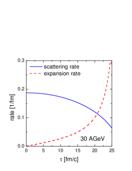
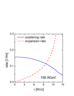
Figure 2: Comparison of the kaon scattering rate calculated according to Eq. (24) and the expansion rate introduced in Eq. (2) as a function of time for three scenarios which fit the data at: 11.6 $A$GeV (left), 30 $A$GeV (middle), and 158 $A$GeV (right).

They are typically of the order 0.1 fm^-1; somewhat larger at higher density in the beginning and smaller at later times. With thermal kaon velocity of about $0.7\,c$ this leads to a mean free path of 7 fm. Even if the kaon moved with light velocity, like some primordially produced kaons, the mean free path would still come to about 10 fm. This length is comparable to the size of a fireball. Would the kaon mean free path be much bigger than the size of a fireball, one could assume kaons to escape from the system right after the production event without any further scattering. Oppositely, a mean free path much smaller than the fireball size would indicate that kaons rescatter intensively and stay in thermal equilibrium with fireball medium. Reality is somewhere in between these two limits. In any case, they do not simply escape from the fireball. In our type of model we can only make two extreme assumptions: decouple the produced kaons from the system completely or treat them all as a part of the system. Due to a chance of absorption the latter appears closer to reality. For practical reason, in calculation of kaon scattering and annihilation rates thermally equilibrated velocity distributions have been assumed.

Let us also note that the inverse slope parameters $T^{*}$ of kaon spectra, together with pions and protons seem to follow the empirical prescription $T^{*}=T+m\langle v_{t}\rangle^{2}$, where $\langle v_{t}\rangle^{2}$ is average transverse expansion velocity na57 . This suggests that all these species freeze-out kinematically at the same time.

The influence of our simplification is twofold. Firstly, we may overestimate the amount of kaons that are annihilated. Secondly, the energy which the kaons carry is not taken out of the system as it would be so if kaons decouple.

The overestimation of kaon annihilation would introduce only small error if the annihilation rate is small compared to the production rate. The rates are plotted for three typical scenarios in Fig. 3 (same scenarios as in Fig. 2).

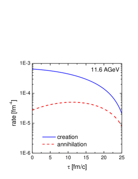
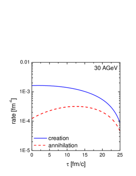
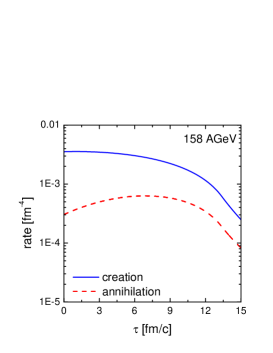
Figure 3: Comparison of total kaon creation and annihilation rates as a function of time for three scenarios which fit the data at: 11.6 $A$GeV (left), 30 $A$GeV (middle), and 158 $A$GeV (right).

The annihilation rate grows since the kaon abundance increases. Originally it is smaller than the creation rate by an order of magnitude, at late times by a factor of 2. From the fact that up to 50% of final state direct kaons are produced primordially and not due to kaon creation modelled here (see Fig. 12), we conclude that a decrease of the (small) annihilation rate would not change our results too much. At most, it would slightly shorten the lifetimes necessary to describe the data.

In order to estimate a possible error in the total energy of the fireball we plot in Fig. 4 the ratio of the energy carried by thermal kaons to the total energy of the system.

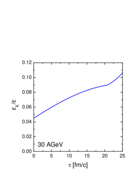
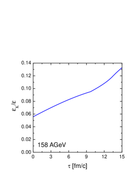
Figure 4: Ratios of the energy contained in kaons to the total energy of the system as functions of time for three scenarios which fit the data at: 11.6 $A$GeV (left), 30 $A$GeV (middle), and 158 $A$GeV (right).

At the beginning, at most 6% of energy is contained in kaons. This is the part of energy we should take away if we treat primordial kaons as non-interacting. Since energy density goes roughly with the fourth power of temperature, $T$ would not change much and the production rates would stay practically unchanged. In general, subtracting a few per cent from the energy density would have small influence on chemical composition because at the same time we would not include kaons and the available energy would be distributed among smaller number of degrees of freedom, thus changing the temperature only little.

It is possible to refine our treatment of kaons as a part of the fireball by comparing the kaon scattering rate to the expansion rate of the fireball, cf. Fig. 2. At the beginning of fireball evolution, expansion rate is lower than the scattering rate, thus we say that kaons are thermally equilibrated. When the expansion rate becomes comparable or bigger than the scattering rate, this means that the density of fireball drops considerably before a kaon had a chance to scatter. Then kaons are assumed to decouple from thermal equilibrium. Decoupling is a gradual process but we cannot treat it so in the framework of our model. We say that the kaons decouple at once when

$$-\frac{1}{\rho_{B}}\,\frac{d\rho_{B}}{d\tau}\geq\theta\,{\cal R}_{\rm scatt}\,.$$ (25)

When this condition becomes fulfilled, we fix the temperature for kaons in eq. (22e). We thus assume that the kaons keep a higher temperature than other species, because they decoupled from the thermal bath earlier. By default, the constant $\theta$ is set to 1, though no exact value can be specified by theory bgz ; fow . Variations of $\theta$ turn out to have negligible influence on the results.

In Fig. 2 we demonstrate that the decoupling according to this prescription happens only towards the end of expansion.

II.4 A summary of the evolution procedure

For an easier overview, we summarize the algorithm for time evolution. Suppose, at time $\tau$ we know all quantities: $\varepsilon$, $\rho_{B}$, $\rho_{3}$, all kaon densities, and thermodynamic quantities $T$, $\mu_{B}$, $\mu_{3}$, $\gamma_{S}$, and all $\gamma_{i}$’s. We proceed to time $\tau+d\tau$ in following steps:

1. Calculate new densities of $K^{+}$, $K^{0}$, $K^{*+}$, $K^{*0}$ from eq. (4).

2. Calculate total kaon scattering rate ${\cal R}_{\rm scatt}$ from eq. (24).

3. Obtain $\varepsilon$, $\rho_{B}$, $\rho_{3}$ from prescription (8). Also obtain expansion rate from eq. (9).

4. Determine $\rho_{S}$ from eq. (21).

5. Decide by the use of inequality (25) if kaons are thermalized according.

6. Obtain $T$, $\mu_{B}$, $\mu_{3}$, $\gamma_{S}$, and $\gamma_{i}$’s from numerically inverting relations (22). If kaons are not thermalized, fix their temperature in eq. (22e).

7. Calculate the density of any desired species via

   $$\rho_{i}=\frac{1}{2\pi^{2}}\,g_{i}\,\lambda_{i}\,m_{i}^{2}\,T\,K_{2}\left(\frac{m_{i}}{T}\right)$$ (26)

   for non-strange species, and

   $$\rho_{i}=\frac{1}{2\pi^{2}}\,g_{i}\,\lambda_{i}\,\gamma_{S}^{|S_{i}|}\,m_{i}^{2}\,T\,K_{2}\left(\frac{m_{i}}{T}\right)$$ (27)

   for species with $S<0$.

8. Continue to next time step by going to step 1.

In the outlined setup of the model there are different handles to tune the final $K^{+}$ density and those of $K^{-}$ and $\Lambda$. All these, normalized by pion densities, will be compared to data. Since the production of $K^{+}$ is calculated explicitly, its density depends on temperature and time. If we can reproduce the $\langle K^{+}\rangle/\langle\pi^{+}\rangle$ ratio, this means that we have gotten the total strangeness production right. The strange quarks are then distributed among $K^{-}$, $\Lambda$, and other species according to the temperature and chemical potentials. Thus the key to simultaneous fit to $\langle K^{-}\rangle/\langle\pi^{-}\rangle$ and $\langle\Lambda\rangle/\langle\pi\rangle$ ratios is the correct value of the temperature.

II.5 Final state and feed-down from resonance decays

Chemical composition of the final state in Au+Au collisions at beam energy 11.6 $A$GeV b23 ; b24 ; b25 ; b26 ; bcksr and Pb+Pb collisions at beam energies 30 AGeV alt20 , 40, 80, and 158 $A$GeV ktpdata have been analyzed in the framework of the statistical hadronization model complemented by strangeness suppression factor $\bar{\gamma}_{S}$ by Becattini and collaborators becatt . We use their results on temperature, chemical potentials and $\bar{\gamma}_{S}$ in order to characterize the state of chemical freeze-out which we aim for.

Table 1: Thermodynamic quantities and densities characterising the chemical freeze-out state in collisions at different energies. Values of $T$, $\mu_{B}$, $\mu_{3}$, $\mu_{S}$, and $\bar{\gamma}_{S}$ from becatt serve as an input in reconstructing the final state values of $\epsilon_{f}$, $\rho_{B\,f}$ and $\rho_{3\,f}$.

$E_{\rm beam}$ [$A$GeV]	11.6	30	40	80	158
$T$ [MeV]	118.1	139.0	147.6	153.7	157.8
$\mu_{B}$ [MeV]	549.1	423.1	375.1	293.6	243.7
$\mu_{3}$ [MeV]	–11.8	–11.0	–10.3	–8.2	–7.1
$\mu_{S}$ [MeV]	117.5	99.1	90.5	69.7	59.2
$\bar{\gamma}_{S}$	0.652	0.938	0.757	0.73	0.843
$\varepsilon_{f}$ [GeV/fm3]	0.132	0.173	0.203	0.194	0.198
$\rho_{Bf}$ [fm-3]	0.086	0.087	0.091	0.068	0.058
$\rho_{3f}$ [fm-3]	–0.0083	–0.0097	–0.0102	–0.0079	–0.0070

Thus obtain the final state value of the energy density, $B$ and $I_{3}$ densities (Table 1). These are three of the parameters which specify the time evolution. Note that even fixing the final state densities does not guarantee that we arrive at the correct final chemical composition because final temperature depends on the amount of produced strangeness which is calculated kinetically. On the other hand, it is important to realize that if we end up in a state with the correct amount of kaons and the correct final energy and baryon densities guaranteed by construction, then we also reproduce the temperature as inferred in chemical freeze-out fits in becatt and therefore all ratios of abundances, i.e. also those involving only non-strange species. If we then compare calculated density of one of the species to the total measured multiplicity of that species we could infer the volume and thus multiplicities of all other species.

A significant portion of final state pions stems from decays of resonances. These must be included when obtaining ratios of multiplicities. This is done by determining the number of resonances and multiplying by the average number of pions produced in a decay of one resonance. Also, there is feed-down to kaon production from $K^{*}$ decays and to the number of $\Lambda$’s from other strange baryons. A list of all contributions is provided in Appendix C.

II.6 Initial state

Now we have to specify the initial conditions for the evolution equation (4). Note that strangeness is also produced in primordial collisions of incident nucleons. The amount will be extrapolated from strangeness abundance in nucleon-nucleon interactions. We shall equate the ratio of $K^{+}$ density and the density of negative hadrons to the ratios of multiplicities $\langle K^{+}\rangle_{NN}/\langle h^{-}\rangle_{NN}$ extrapolated from nucleon-nucleon collisions. The values are summarized in Table 2.

Table 2: Mean multiplicity $\langle K^{+}\rangle_{NN}$ from nucleon-nucleon collisions and ratios $\langle K^{+}\rangle_{NN}/\langle h^{-}\rangle_{NN}$ extrapolated to a mixture of protons and neutrons corresponding to Au+Au or Pb+Pb collisions at indicated beam energies.

	$\langle K^{+}\rangle_{NN}$	$\frac{\langle K^{+}\rangle_{NN}}{\langle h^{-}\rangle_{NN}}$
Au+Au @ 11.6 AGeV	$0.0607\pm 0.0252$	0.0581
Pb+Pb @ 30 AGeV	$0.143\pm 0.027$	0.0821
Pb+Pb @ 40 AGeV	$0.163\pm 0.036$	0.0842
Pb+Pb @ 80 AGeV	$0.218\pm 0.059$	0.0880
Pb+Pb @ 158 AGeV	$0.272\pm 0.056$	0.0883

Density of $K^{0}$ is then determined as $\rho_{K^{0}}=\rho_{K^{+}}\exp(-\mu_{3}/T)$. No $K^{*}$’s are assumed in the initial state. Species with $S<0$ must balance the total strangeness to 0 and are set into relative chemical equilibrium. We describe the choice of the initial state in detail in Appendix D.

III Results and discussion

We calculated the resulting $\langle K^{+}\rangle/\langle\pi^{+}\rangle$, $\langle K^{-}\rangle/\langle\pi^{-}\rangle$ and $\langle\Lambda\rangle/\langle\pi\rangle$ ratios for many different evolution scenarios for the beam energies 11.6 $A$GeV (Au+Au), and 30, 40, 80, 158 $A$GeV (Pb+Pb). Thus we explore the region of the peak in $\langle K^{+}\rangle/\langle\pi^{+}\rangle$.

At every beam energy the investigated scenarios differ by the initial energy density and total lifetime of the fireball. The final configurations listed in Table 1 are fixed from the analysis becatt . The range of initial energy densities goes up to 3.0 GeV/fm³. This seems to surpass the critical value for deconfinement indicated by lattice calculations. We have two comments here, however: first, the system under investigation is out of equilibrium and it is a question whether results of equilibrium statistical physics can be applied here. The relaxation time is not known. Second, an uncertainty in determination of the critical temperature was reported at the Quark Matter 2005 conference katz leading to a value higher than one previously used.

The parameter $\tau_{0}$ is chosen such that it is smaller than the total lifetime by 7 fm/$c$, $\tau_{0}=\tau_{T}-7{\rm fm}/c$. Such a value is motivated by measurement of the longitudinal HBT radius $R_{l}$, which—in a Bjorken scenario—indicates that the thermal freeze-out happens about 8-9 fm/$c$ after the reference $\tau_{0}$. As we deal in our study with chemical freeze-out, we set $\tau_{T}-\tau_{0}$ a little smaller.

Since we know from transverse momentum spectra and HBT radius anlyses that there is considerable transverse expansion, we fix $\alpha=2$. The equation of state is set by a modest value of $\kappa=1/6$, or $\delta=6/7$.

The last parameter to specify is ${\cal R}_{\rm max}$. If we fix the initial and final densities and the total lifetime in which the fireball evolves between these two states, there is only a limited range of values the maximum expansion rate can assume. For every pair of chosen initial energy density and lifetime we explored the two limiting values of ${\cal R}_{\rm max}$. It turned out that the differences due to selection of ${\cal R}_{\rm max}$ in the studied ratios were of the order 10%.

The results are plotted in Figs. 5-9.

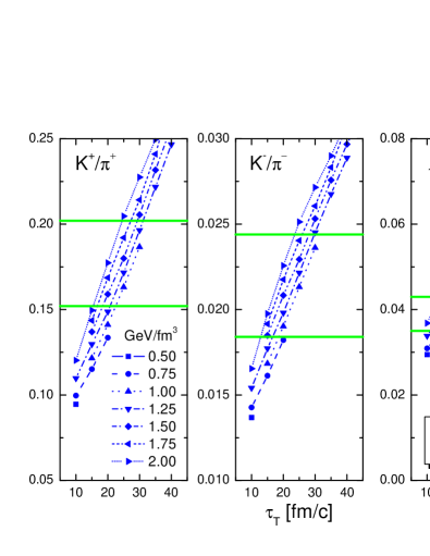
Figure 5: Ratios $\langle K^{+}\rangle/\langle\pi^{+}\rangle$, $\langle K^{-}\rangle/\langle\pi^{-}\rangle$, and $\langle\Lambda\rangle/\langle\pi\rangle$ as a function of the total lifetime of the system, calculated for Au+Au collisions at beam energy of 11.6 $A$GeV. Different curves correspond to different initial energy densities. Horizontal lines indicate 1$\sigma$ intervals around the measured data.

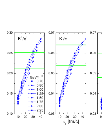
Figure 6: Ratios $\langle K^{+}\rangle/\langle\pi^{+}\rangle$, $\langle K^{-}\rangle/\langle\pi^{-}\rangle$, and $\langle\Lambda\rangle/\langle\pi\rangle$ as a function of the total lifetime of the system, calculated for Pb+Pb collisions at beam energy of 30 $A$GeV. Different curves correspond to different initial energy densities. Horizontal lines indicate 1$\sigma$ intervals around the measured data.

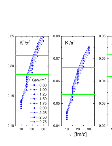
Figure 7: Ratios $\langle K^{+}\rangle/\langle\pi^{+}\rangle$, $\langle K^{-}\rangle/\langle\pi^{-}\rangle$, and $\langle\Lambda\rangle/\langle\pi\rangle$ as a function of the total lifetime of the system, calculated for Pb+Pb collisions at beam energy of 40 $A$GeV. Different curves correspond to different initial energy densities. Horizontal lines indicate 1$\sigma$ intervals around the measured data.

Figure 8: Ratios $\langle K^{+}\rangle/\langle\pi^{+}\rangle$, $\langle K^{-}\rangle/\langle\pi^{-}\rangle$, and $\langle\Lambda\rangle/\langle\pi\rangle$ as a function of the total lifetime of the system, calculated for Pb+Pb collisions at beam energy of 80 $A$GeV. Different curves correspond to different initial energy densities. Horizontal lines indicate 1$\sigma$ intervals around the measured data.

Figure 9: Ratios $\langle K^{+}\rangle/\langle\pi^{+}\rangle$, $\langle K^{-}\rangle/\langle\pi^{-}\rangle$, and $\langle\Lambda\rangle/\langle\pi\rangle$ as a function of the total lifetime of the system, calculated for Pb+Pb collisions at beam energy of 158 $A$GeV. Different curves correspond to different initial energy densities. Horizontal lines indicate 1$\sigma$ intervals around the measured data.

The shown results for energies 30 $A$GeV and upward were obtained for the highest possible ${\cal R}_{\rm max}$. If scenarios with slowest possible ${\cal R}_{\rm max}$ are used, the lifetime needed to reach the same result is prolonged by 1-2 fm/$c$. For the lowest studied energy we used the lowest ${\cal R}_{\rm max}$ scenarios.

In Figs. 5-9 we clearly observe that the resulting multiplicity ratios depend crucially on the total lifetime of the fireball. Dependence on the initial energy density is less important. The latter is more strongly pronounced at lower energies, where the baryon density is higher. Since the dependence on the energy density is so weak, we do not expect a major change in the results if parameterization for time dependence of the energy density was changed.

In order to quantify the agreement between our calculations and experimental data, for every examined scenario we calculate the standard $\chi^{2}$ measure

$$\chi^{2}=\sum_{i}\frac{(\mbox{theory}_{i}-\mbox{data}_{i})^{2}}{\mbox{error}_{i}^{2}}\,,$$ (28)

where the sum runs over the three measured data points for every beam energy: $\langle K^{+}\rangle/\langle\pi^{+}\rangle$, $\langle K^{-}\rangle/\langle\pi^{-}\rangle$, $\langle\Lambda\rangle/\langle\pi\rangle$. The resulting $\chi^{2}$ values are summarized in Fig. 10.

Figure 10: The quality-of-fit measure $\chi^{2}$, as defined in eq. (28) as a function of the total lifetime. Different panels correspond to different beam energies and various curves to different initial energy densities.

For beam energies above 30 $A$GeV the best agreement with data is indeed obtained if the lifetime decreases as a function of beam energy. At the highest AGS energy, our model fits data best if the lifetime is shorter than at 30 $A$GeV. In some sense we have translated the non-trivial excitation function of $\langle K^{+}\rangle/\langle\pi^{+}\rangle$ into the dependence of the lifetime on the collision energy. A maximum of the lifetime at 30 $A$GeV could be an indicator of some change in evolution dynamics, e.g. a soft point in the equation of state leading to a low pressure gradient and a prolonged lifetime. However, we can not insist on such conclusion here, since comparison with data cannot clearly exclude that a lifetime at beam energy 11.6 $A$GeV is as long as at 30 $A$GeV. A slight change in the dependence of $\tau_{T}$ on the collision energy, could be expected if other time evolution parameterizations is used.

In Table 3 we present the most favorable sets of the evolution parameters. We choose those sets where the fireball lifetime does not increase with an increasing beam energy. Corresponding final densities are given in Table 1. Our results for the ratios $\langle K^{+}\rangle/\langle\pi^{+}\rangle$, $\langle K^{-}\rangle/\langle\pi^{-}\rangle$, and $\langle\Lambda\rangle/\langle\pi\rangle$ are shown in Fig. 11.

Table 3: Parameters of the simulations which lead to results compared to data in Fig. 11. In the lower two rows we compare the chemical freeze-out temperature $T$ obtained by Becattini et al. becatt with the teperature $T_{f}$ we obtain in our simulations.

$E_{\rm beam}$ [$A$GeV]	11.6	30	40	80	158
$\varepsilon_{0}$ [GeV/fm3]	1	1.5	2	2.25	2.75
$\tau_{T}$ [fm/$c$]	25	25	20	15	15
${\cal R}_{\rm max}$ [fm-1]	0.286	0.305	0.333	0.379	0.374
$T$ [MeV]	118.1	139.0	147.6	153.7	157.8
$T_{f}$ [MeV]	114.7	134.1	143.3	149.3	153.6

Figure 11: Comparison of our results with data alt20 ; ktpdata . Calculations were performed with parameters listed in Tables 1 and 3.

In Table 3 we see that the final state temperature agrees rather well with the results of chemical freeze-out fits by Becattini et al. becatt . Note that we did not perform a calculation at the beam energy 20 $A$GeV due to lack of final state analysis from this collision energy in becatt .

Table 3 and Fig. 11 are the main results of our study. In the subsequent subsections we illustrate the time evolution of various densities and rates.

III.1 The evolution

Evolution of kaon density in Pb+Pb collisions at 30 $A$GeV is illustrated in Fig. 12 (left panel).

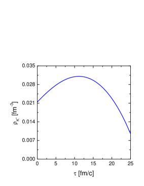
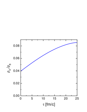
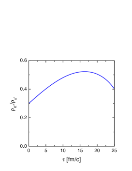
Figure 12: Left panel: evolution of the kaon densities. Middle panel: evolution of the kaon density divided by the baryon number density. Right panel: evolution of the ratio $\rho_{K^{+}}/\rho_{\pi^{+}}$.

The growth of $\rho_{K^{+}}$ is soon overrun by the decrease due to expansion. To cancel the expansion effect we have to normalize the kaon density by the baryon density. The latter, being density of a conserved charge, changes due to expansion only.

The ratio $\rho_{K^{+}}/\rho_{B}$ (middle panel in Fig. 12) shows a steady increase in time. The ratio of $\rho_{K^{+}}/\rho_{\pi^{+}}$ (right panel in Fig. 12) finishes with rather high value which does not correspond to the measured $\langle K^{+}\rangle/\langle\pi^{+}\rangle$. The final result which does reproduce the data includes, however, feed-down from resonance decays which contribute largely to pion production.

In Fig. 13 we show the density evolution for some other species.

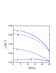
Figure 13: Densities of $\pi^{+}$, $p$, $\rho^{+}$, $\Lambda$, and $K^{-}$ as functions of time for the scenario which reproduces 30 $A$GeV data. In the lower panel the densities are normalized to the baryon density.

When the densities are normalized to baryon density in order to get rid of the effect of expansion we clearly see that due to cooling the relative abundance of pions and nucleons as the lightest mesons and baryons increases with respect to other species. Normalized $K^{-}$ and $\Lambda$ densities rise continuously in time.

III.2 The rates

Kaons are produced in various reactions. In Fig. 14 we show the production rates of different reactions as functions of time.

Figure 14: Production rates of $K^{+}$ due to selected processes as a function of time for three scenarios which fit the data at: 11.6 $A$GeV (left), 30 $A$GeV (middle), and 158 $A$GeV.

The three shown examples refer to scenarios which reproduce data for 11.6, 30, and 158 $A$GeV in Fig. 11. As expected, due to an increase of the energy density the production rates grow with increasing beam energy. In all cases, the dominant contribution is due to $\pi\pi$ reactions. A very important contribution comes from reactions of pions with hyperons. Recall that the corresponding cross section is not known experimentally and we chose a constant matrix element for this reaction. This introduces some uncertainty into our quantitative results. Note however that since the contribution from $\pi Y$ reactions has almost always the same relative importance in comparison to $\pi\pi$ reactions, we do not expect any qualitative change of our results under modification of $\pi Y$ cross sections.

There is a clear change when moving from lower, baryon-dominated, energies toward higher, meson-dominated energies. While at 11.6 $A$GeV the second largest contribution comes from $\pi N$ reactions, the contribution from this type of reactions decreases with increasing beam energy and actually becomes even lower than $\pi\rho$ contribution at 158 $A$GeV.

We study the meson-meson production rates together with $\pi N$, $\pi Y$ and $N\Delta$ rate as a function of temperature in Fig. 15.

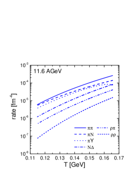
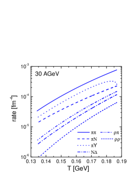
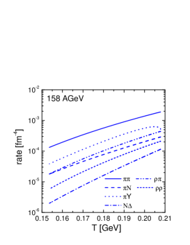
Figure 15: Production rates of $K^{+}$ from selected reaction processes as a function of temperature for three scenarios which fit the data at: 11.6 $A$GeV (left), 30 $A$GeV (middle), and 158 $A$GeV.

As mentioned, the difference between the three different panels in in baryon density. The $\pi\pi$ rate becomes relatively more and more important. As it is outlined in Appendices B.7 and B.8, we took a great care in determining the $\pi\rho$ and $\rho\rho$ cross sections. Note that we do not treat all meson-meson cross section as being the same, in contrast to HSD ; mosel . The resulting suppression in $\pi\rho$ channel is due to $p$-wave suppression of the reaction $\pi\rho\to\phi\to K\bar{K}$ and a higher threshold in the channel $\pi\rho\to K\bar{K}^{*}$. The later cross section was determined from the scattering amplitudes following from the covariant solution of the Bethe-Salpeter equation LK with the leading chiral order Weinberg-Tomozawa term as an interaction kernel. The untarization effects are found to be important leading to a smaller cross section than what would be inferred from $\pi\pi$ cross section. The $\rho\rho$ rate is suppressed thermally due to large mass of the $\rho$ mesons, and the resulting contribution is very low.

IV Conclusions

In the introduction we motivated our study by the question whether it is possible to rule out any hadronic interpretation of the observed excitation function of $\langle K^{+}\rangle/\langle\pi^{+}\rangle$, $\langle K^{-}\rangle/\langle\pi^{-}\rangle$, and $\langle\Lambda\rangle/\langle\pi\rangle$ ratios. We proposed a non-equilibrium hadronic model which is able to reproduce the data by virtue of varying the total lifespan of a fireball at different energies.

Thus one has to do more in trying to exclude this kind of models. Another indications of non-trivial effects in the region of the $\langle K^{+}\rangle/\langle\pi^{+}\rangle$ peak is a step in kaon spectra inverse slopes, and a change in the pion yield per participant. The model must be tested on these observables, as well.

Our findings are based on the assumption that the lifetime of a fireball becomes shorter as one moves to higher beam energies. We want to stress that most of the information we have about the space-time evolution of a fireball comes from hadronic spectra and correlations, which are formed at the freeze-out stage of fireball evolution. This is just the final state to which many possible evolution scenarios may lead. One of the future tasks should be a careful check how hadronic observables calculated within our model fit the data. This is rather involved project. Although we were lead by the data in formulating our model, we refrained from such detailed and careful fits here.

The whole duration of fireball evolution is reflected in penetrating probes like dilepton spectra. Their measurement was improved dramatically in the last years ceres ; ceres40 ; na60 . It seems to be crucial, therefore, to check our model assumption about the lifetime against the dilepton spectra.

Our approach addressed here only a part of the whole problem by asking how do different fireball evolution scenarios influence the data. We ignored the question how a specific evolution scenario follows from the microscopic properties of the created matter? This question must be, of course, addressed in the future if the model survives all experimental tests. On the other hand, if we succeed to exclude the model on a set of data, there will be no need to answer this question. This approach might be simpler to begin with.

Appendix A Parameters of the time dependence ansatz

Here we express the parameters of eqs. (8) in terms of $\varepsilon_{0}$, $\tau_{T}$, $\varepsilon_{f}$, $\rho_{Bf}$, $\rho_{3f}$, $\tau_{0}$, $\alpha$, and ${\cal R}_{\rm max}$, which were introduced in Section II.1.

The easiest to obtain are $\varepsilon_{0}^{\prime}$, $\rho_{B0}^{\prime}$, $\rho_{30}^{\prime}$

$$\varepsilon_{0}^{\prime} = \varepsilon_{f}\,(\tau_{T}-\tau_{0})^{\alpha/\delta}$$ (29a)

$$\rho_{B0}^{\prime} = \rho_{Bf}\,(\tau_{T}-\tau_{0})^{\alpha}$$ (29b)

$$\rho_{30}^{\prime} = \rho_{3f}\,(\tau_{T}-\tau_{0})^{\alpha}$$ (29c)

Since the expansion rate at time $\tau_{s}$ must be ${\cal R}_{\rm max}$, from eq. (9) we see

$$\tau_{s}=\frac{\alpha}{{\cal R}_{\rm max}}+\tau_{0}\,.$$ (30)

Parameters $a$ and $b$ are obtained from matching at time $\tau_{s}$

$$\varepsilon_{0}(1-a\tau_{s}-b\tau_{s}^{2}) = \frac{\varepsilon_{0}^{\prime}}{(\tau_{s}-\tau_{0})^{\alpha/\delta}}$$ (31a)

$$\varepsilon_{0}(1+2b\tau_{s}) = \frac{\alpha\,\varepsilon_{0}^{\prime}}{\delta(\tau_{s}-\tau_{0})^{\alpha/\delta-1}}$$ (31b)

which lead to

$$a = \frac{2}{\tau_{s}}$$ (32a)

$$-\frac{\varepsilon_{f}}{\varepsilon_{0}}\,\left(\frac{2}{\tau_{s}}+\frac{\alpha}{\delta(\tau_{s}-\tau_{0})}\right)\,\left(\frac{\tau_{T}-\tau_{0}}{\tau_{s}-\tau_{0}}\right)^{\alpha/\delta}$$

$$b = \frac{\varepsilon_{f}}{\varepsilon_{0}}\,\left(\frac{1}{\tau_{s}^{2}}+\frac{\alpha}{\delta\tau_{s}(\tau_{s}-\tau_{0})}\right)\left(\frac{\tau_{T}-\tau_{0}}{\tau_{s}-\tau_{0}}\right)^{\alpha/\delta}$$ (32b)

$$-\frac{1}{\tau_{s}^{2}}\,.$$

For $B$ and $I_{3}$ densities we obtain from matching at $\tau_{s}$

$$\rho_{B0} = \frac{\rho_{Bf}}{(1-a\tau_{s}-b\tau_{s}^{2})^{\delta}}\,\left(\frac{\tau_{T}-\tau_{0}}{\tau_{s}-\tau_{0}}\right)^{\alpha}$$ (33a)

$$\rho_{30} = \frac{\rho_{3f}}{(1-a\tau_{s}-b\tau_{s}^{2})^{\delta}}\,\left(\frac{\tau_{T}-\tau_{0}}{\tau_{s}-\tau_{0}}\right)^{\alpha}\,.$$ (33b)

In Table 4 we present the values of parameters $a$, $b$ and $\tau_{s}$ corresponding to the energy density, fireball lifetime and $\mathcal{R}_{\rm max}$ given in Table 3

Table 4: Parameters of the time dependence (8) corresponding to the energy density, fireball lifetime and $\mathcal{R}_{\rm max}$ given in Table 3.

$E_{\rm beam}$ [$A$GeV]	11.6	30	40	80	158
$a\times 10^{4}$ [fm-1]	$142.6$	$5.482$	$4.963$	$10.77$	$8.448\cdot 10^{-2}$
$b\times 10^{4}$ [fm-2]	$7.752$	$13.29$	$21.55$	$41.60$	$44.70$
$\tau_{s}$ [fm/$c$]	25.00	24.56	19.01	13.28	12.98

Appendix B Cross sections for kaon production

In this section we specify the cross sections of all reactions with strangeness production which are relevant at the collision energies under consideration. We disregard a possible modification of cross sections in dense and hot nuclear matter and accept their vacuum forms. This approximation complies with our assumption above that properties of all particles do not change in medium either.

For processes with two particles in the final state the inverse reactions are included in the calculation, as well. The cross section for the inverse reactions follows from phase-space considerations as

$$\sigma_{34\to 12}(\sqrt{s}) = \frac{(2J_{3}+1)(2J_{4}+1)}{(2J_{1}+1)(2J_{2}+1)}\,\frac{p^{2}_{\rm cm}(s,m_{1},m_{2})}{p^{2}_{\rm cm}(s,m_{3},m_{4})}\,$$ (34)

$$\times \sigma_{12\to 34}(\sqrt{s})\,,$$

where $J_{i}$ and $m_{i}$ are spins and masses of the participating species, and $p_{\rm cm}$ is the center-of-mass momentum defined as

$$p^{2}_{\rm cm}(s,m_{a},m_{b}) = {\frac{[s-(m_{1}^{2}+m_{2}^{2})]^{2}-4\,m_{1}^{2}\,m_{2}^{2}}{4\,s}}\,.$$ (35)

In all parameterizations below, energy units will be GeV and cross sections are measured in millibarns.

B.1 Reactions of $\pi+N$

Cross sections for $\pi N\to K^{+}\Lambda$ are all related by isospin symmetry kujon to $\pi^{0}n\to K^{0}\Lambda$, which we take from tsau

$$2\sigma(\pi^{0}p\to K^{+}\Lambda) = \sigma(\pi^{+}n\to K^{+}\Lambda)=\sigma(\pi^{-}p\to K^{0}\Lambda)=2\sigma(\pi^{0}n\to K^{0}\Lambda)=\frac{0.007665(\sqrt{s}-1.613)^{0.1341}}{(\sqrt{s}-1.720)^{2}+0.007826}\,.$$ (36)

In Fig. 16 we compare this parameterization of the $\pi^{+}p\to K^{0}\Lambda$ reaction with the available experimental data.

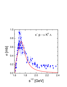
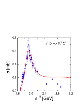
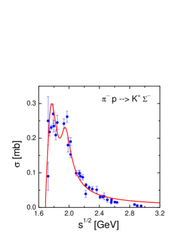
Figure 16: Total cross section of the $\pi^{+}p\to K^{0}\Lambda$, $\pi^{+}p\to K^{+}\Sigma^{+}$, and $\pi^{-}p\to K^{+}\Sigma^{-}$ reactions: solid line calculated with eq. (36), dots are the experimental data from Ref. expdata

¿From tsu we get the $\pi N\to\Sigma K^{+}$ cross sections

$$\sigma(\pi^{+}p\to K^{+}\Sigma^{+})=\,\sigma(\pi^{-}n\to K^{0}\Sigma^{-}) = \frac{0.03591(\sqrt{s}-1.688)^{0.9541}}{(\sqrt{s}-1.890)^{2}+0.01548}+\frac{0.1594(\sqrt{s}-1.688)^{0.01056}}{(\sqrt{s}-3.000)^{2}+0.9412}\,,$$ (37)

$$\sigma(\,\pi^{0}p\to K^{+}\Sigma^{0}\,)=\,\sigma(\,\pi^{0}n\to K^{0}\,\Sigma^{0}\,) = \frac{0.003978(\sqrt{s}-1.688)^{0.5848}}{(\sqrt{s}-1.740)^{2}+0.00667}+\frac{0.04709(\sqrt{s}-1.688)^{2.1650}}{(\sqrt{s}-1.905)^{2}+0.006358}\,,$$ (38)

$$\sigma(\pi^{-}p\to K^{+}\Sigma^{-})=\,\sigma(\pi^{+}n\to K^{0}\Sigma^{+}) = \frac{0.009803(\sqrt{s}-1.688)^{0.6021}}{(\sqrt{s}-1.742)^{2}+0.006583}+\frac{0.006521(\sqrt{s}-1.688)^{1.4728}}{(\sqrt{s}-1.940)^{2}+0.006248}\,,$$ (39)

$$\sigma(\pi^{+}n\to K^{+}\Sigma^{0})=\sigma(\pi^{-}p\to K^{0}\Sigma^{0})=\sigma(\pi^{0}n\to K^{+}\Sigma^{-})=\sigma(\pi^{0}p\to K^{0}\Sigma^{+})=\frac{0.05014(\sqrt{s}-1.688)^{1.2878}}{(\sqrt{s}-1.730)^{2}+0.006455}\,.$$ (40)

The quality of these parameterizations is demonstrated in Fig. 16 for $\pi^{+}p\to K^{+}\Sigma^{+}$, and $\pi^{-}p\to K^{+}\Sigma^{-}$ reactions.

Reactions $\pi N\to NK\bar{K}$ were studied in Ref. cassing . It was found that under assumption that main contribution to the $\pi N\to NK\bar{K}$ reaction is given by the diagram

(41)

all different isospin channels can be parameterized as

$$\bar{\sigma}(\pi_{a}N_{b}\to N_{c}K_{d}\bar{K}_{e})=c\,1.121\,\left[1-\frac{s_{0}}{s}\right]^{1.86}\!\left[\frac{s_{0}}{s}\right]^{2}\!,$$ (42)

where $\sqrt{s_{0}}=m_{N}+2m_{K}=1.929$ GeV and $c$ is a channel dependent isospin coefficient. The latter ones are collected Table 5. In Figs. 17 and 18 we confront these parameterizations with the available experimental data.

Table 5: Isospin coefficient in the parameterization (42) of $\pi N\to NK\bar{K}$ reactions

reaction	$c$		reaction	$c$
$\pi^{+}p\to pK^{+}\bar{K}^{0}$	1		$\pi^{-}p\to pK^{0}K^{-}$	1
$\pi^{+}n\to pK^{0}\bar{K}^{0}$	2		$\pi^{-}p\to nK^{0}\bar{K}^{0}$	2
$\pi^{+}n\to pK^{+}K^{-}$	2		$\pi^{-}p\to nK^{+}K^{-}$	2
$\pi^{+}n\to nK^{+}\bar{K}^{0}$	1		$\pi^{0}n\to pK^{0}K^{-}$	2
$\pi^{0}p\to pK^{0}\bar{K}^{0}$	$\frac{1}{2}$		$\pi^{0}n\to nK^{0}\bar{K}^{0}$	$\frac{1}{2}$
$\pi^{0}p\to pK^{+}K^{-}$	$\frac{1}{2}$		$\pi^{0}n\to nK^{+}K^{-}$	$\frac{1}{2}$
$\pi^{0}p\to nK^{+}\bar{K}^{0}$	2		$\pi^{-}n\to nK^{0}K^{-}$	1

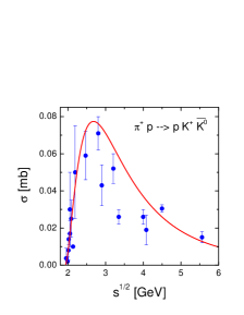
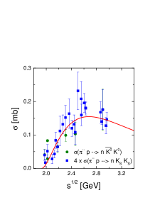
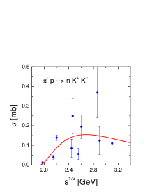
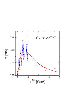
Figure 17: Total cross section of the $\pi^{+}p\to pK^{+}\bar{K^{0}}$, $\pi^{-}p\to nK^{0}\bar{K}^{0}$, $\pi^{-}p\to nK^{+}K^{-}$, and $\pi^{-}p\to pK^{0}K^{-}$ reactions: solid line calculated with eq. (42), dots are the experimental data from Ref. expdata

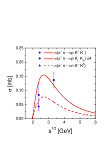
Figure 18: Total cross section of the $\pi^{+}n\to pK^{+}K^{-}$, $\pi^{+}n\to pK^{0}\bar{K}^{0}$, and $\pi^{+}n\to nK^{+}\bar{K}^{0}$ reactions: solid line calculated with eq. (42), dots are the experimental data from Ref. expdata . Note that isospin symmetry of the diagram (41) predicts that cross sections for $\pi^{+}n\to pK^{+}K^{-}$ and the one for $\pi^{+}n\to pK^{0}\bar{K}^{0}$ multiplied by 4 are same.

B.2 Reactions of $\pi+\Delta$

The cross sections for $\pi\Delta\to YK^{+}$ reactions we take from Ref. tsau

$$\sigma(\pi^{-}\Delta^{++}\to K^{+}\Lambda)=\frac{0.00983(\sqrt{s}-1.613)^{0.7866}}{(\sqrt{s}-1.720)^{2}+0.004852}\,.$$

(43)

The other channels leading to $\Lambda$ production are obtained from isospin symmetry

$$\sigma(\pi^{-}\Delta^{++}\to K^{+}\Lambda) =\sigma(\pi^{+}\Delta^{-}\to K^{0}\Lambda),$$

$$\sigma(\pi^{0}\Delta^{+}\,\,\to K^{+}\Lambda) =\sigma(\pi^{0}\Delta^{0}\to K^{0}\Lambda)$$

$$=\frac{2}{3}\sigma(\pi^{-}\Delta^{++}\to K^{+}\Lambda),$$

$$\sigma(\pi^{+}\Delta^{0}\to K^{+}\Lambda) =\sigma(\pi^{-}\Delta^{+}\to K^{0}\Lambda)$$

$$=\frac{1}{3}\sigma(\pi^{-}\Delta^{++}\to K^{+}\Lambda),$$

For $\pi\Delta\to\Sigma K$ reactions one assumes in tsug that the cross section has a contribution from the isospin $1/2$ channel only. The $I=3/2$ contribution was found small. Then all reactions are related to four isospin combinations parameterized in tsug as:

$$\sigma(\pi^{-}\Delta^{++}\to K^{+}\Sigma^{0})=\frac{0.004959(\sqrt{s}-1.688)^{0.7785}}{(\sqrt{s}-1.725)^{2}+0.008147},$$

$$\sigma(\pi^{0}\Delta^{0}\to K^{+}\Sigma^{-})=\frac{0.006964(\sqrt{s}-1.688)^{0.8140}}{(\sqrt{s}-1.725)^{2}+0.007713},$$

$$\sigma(\pi^{+}\Delta^{0}\to K^{+}\Sigma^{0})=\frac{0.002053(\sqrt{s}-1.688)^{0.9853}}{(\sqrt{s}-1.725)^{2}+0.005414},$$

$$+\frac{0.3179(\sqrt{s}-1.688)^{0.9025}}{(\sqrt{s}-2.675)^{2}+44.88},$$

$$\sigma(\pi^{+}\Delta^{-}\to K^{+}\Sigma^{-})=\frac{0.01741(\sqrt{s}-1.688)^{1.2078}}{(\sqrt{s}-1.725)^{2}+0.003777},$$

For other reactions one finds

$$\sigma(\pi^{0}\Delta^{++}\to K^{+}\Sigma^{+}) =\sigma(\pi^{0}\Delta^{-}\to K^{0}\Sigma^{-})=0,$$

$$\sigma(\pi^{+}\Delta^{+}\to K^{+}\Sigma^{+}) =\sigma(\pi^{-}\Delta^{0}\to K^{0}\Sigma^{-})=0,$$

$$\sigma(\pi^{+}\Delta^{-}\to K^{0}\Sigma^{0}) =\sigma(\pi^{-}\Delta^{++}\to K^{+}\Sigma^{0}),$$

$$\sigma(\pi^{0}\Delta^{+}\to K^{+}\Sigma^{0}) =\sigma(\pi^{0}\Delta^{0}\to K^{0}\Sigma^{0})$$

$$=\frac{1}{3}\sigma(\pi^{+}\Delta^{-}\to K^{+}\Sigma^{-}),$$

$$\sigma(\pi^{-}\Delta^{+}\to K^{0}\Sigma^{0}) =\sigma(\pi^{+}\Delta^{0}\to K^{+}\Sigma^{0}),$$

$$\sigma(\pi^{-}\Delta^{+}\to K^{+}\Sigma^{-}) =\sigma(\pi^{+}\Delta^{0}\to K^{0}\Sigma^{+})$$

$$=\frac{2}{3}\sigma(\pi^{-}\Delta^{++}\to K^{+}\Sigma^{0}),$$

$$\sigma(\pi^{0}\Delta^{+}\to K^{0}\Sigma^{+}) =\sigma(\pi^{0}\Delta^{0}\to K^{+}\Sigma^{-}),$$

$$\sigma(\pi^{-}\Delta^{++}\to K^{0}\Sigma^{+}) =\sigma(\pi^{+}\Delta^{-}\to K^{+}\Sigma^{-}),$$

We also include reactions $\pi\Delta\to NK\bar{K}$. These are taken with the cross section parameterized as in (42). The corresponding isospin constant $c$ follows from the analysis of the diagram (41), where the incoming nucleon line is replaced by the $\Delta$, and depends on incoming and outgoing isospin via Clebsch-Gordan coefficients (cf. eff ). The coefficients are collected in Table 6.

Table 6: Isospin coefficient in the parameterization (42) of $\pi\Delta\to NK\bar{K}$ reactions

reaction	$c$		reaction	$c$
$\pi^{+}\Delta^{+}\,\,\,\,\to pK^{+}\bar{K}^{0}$	2		$\pi^{+}\Delta^{-}\to nK^{+}K^{-}$	3
$\pi^{0}\,\Delta^{++}\to pK^{+}\bar{K}^{0}$	3		$\pi^{+}\Delta^{-}\to nK^{0}\bar{K}^{0}$	3
$\pi^{+}\Delta^{0}\,\,\,\,\,\to pK^{0}\bar{K}^{0}$	1		$\pi^{+}\Delta^{-}\to pK^{0}K^{-}$	0
$\pi^{+}\Delta^{0}\,\,\,\,\,\to pK^{+}K^{-}$	1		$\pi^{0}\,\Delta^{0}\,\to pK^{0}K^{-}$	1
$\pi^{+}\Delta^{0}\,\,\,\,\,\to nK^{+}\bar{K}^{0}$	2		$\pi^{0}\,\Delta^{0}\,\to nK^{0}\bar{K}^{0}$	3
$\pi^{0}\,\Delta^{+}\,\,\,\,\to pK^{0}\bar{K}^{0}$	1		$\pi^{0}\,\Delta^{0}\,\to nK^{+}K^{-}$	1
$\pi^{0}\,\Delta^{+}\,\,\,\,\to pK^{+}K^{-}$	3		$\pi^{-}\Delta^{+}\to nK^{+}K^{-}$	1
$\pi^{0}\,\Delta^{+}\,\,\,\,\to nK^{+}\bar{K}^{0}$	1		$\pi^{-}\Delta^{+}\to nK^{0}\bar{K}^{0}$	1
$\pi^{-}\Delta^{++}\to pK^{0}\bar{K}^{0}$	3		$\pi^{-}\Delta^{+}\to pK^{0}K^{-}$	2
$\pi^{-}\Delta^{++}\to pK^{+}K^{-}$	3		$\pi^{0}\,\Delta^{-}\to nK^{0}K^{-}$	3
$\pi^{-}\Delta^{++}\to nK^{+}\bar{K}^{0}$	0		$\pi^{-}\Delta^{0}\,\to nK^{0}K^{-}$	2

B.3 Reactions of $N+N$

Cross sections for reactions of the type $NN\to N\Lambda K$ and $NN\to N\Sigma K$ are parameterized in tstl . For $NN\to N\Lambda K$ reactions we have

$$\sigma(pp\to p\Lambda K^{+})=\sigma(nn\to n\Lambda K^{0})$$

$$\qquad=1.879\left(\frac{s}{s_{KN\Lambda}}-1\right)^{2.176}\left(\frac{s_{KN\Lambda}}{s}\right)^{5.264}$$

$$\sigma(pn\to n\Lambda K^{+})=\sigma(np\to p\Lambda K^{0})$$

$$\qquad=2.812\left(\frac{s}{s_{KN\Lambda}}-1\right)^{2.121}\left(\frac{s_{KN\Lambda}}{s}\right)^{4.893}$$ (46)

where $s_{KN\Lambda}=(m_{\Lambda}+m_{N}+m_{K})^{2}$ . These parameterizations are confronted with the available experimental data in Fig. 19.

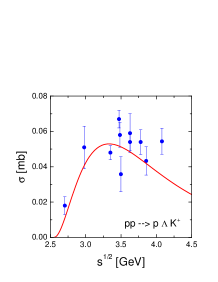
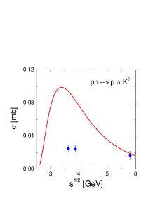
Figure 19: Total cross section of the $pp\to p\Lambda K^{+}$, $pn\to p\Lambda K^{0}$ reactions: solid line calculated with eq. (46), dots are the experimental data from Ref. expdata

For $NN\to N\Sigma K$ reactions we use

$$\sigma(pp\to p\Sigma^{0}K^{+})=\sigma(nn\to n\Sigma^{0}K^{0})$$

$$\qquad=5.321\left(\frac{s}{s_{KN\Sigma}}-1\right)^{2.753}\left(\frac{s_{KN\Sigma}}{s}\right)^{8.510},$$

$$\sigma(pp\to n\Sigma^{+}K^{+})=\sigma(nn\to p\Sigma^{-}K^{0})$$

$$\qquad=1.466\left(\frac{s}{s_{KN\Sigma}}-1\right)^{2.743}\left(\frac{s_{KN\Sigma}}{s}\right)^{3.271},$$

$$\sigma(pn\to p\Sigma^{-}K^{+})=\sigma(np\to n\Sigma^{+}K^{0})$$

$$\qquad=11.02\left(\frac{s}{s_{KN\Sigma}}-1\right)^{2.782}\left(\frac{s_{KN\Sigma}}{s}\right)^{7.674},$$

$$\sigma(pn\to n\Sigma^{0}K^{+})=\sigma(np\to p\Sigma^{0}K^{0})$$

$$\qquad=6.310\left(\frac{s}{s_{KN\Sigma}}-1\right)^{2.773}\left(\frac{s_{KN\Sigma}}{s}\right)^{7.820},$$

$$\sigma(nn\to n\Sigma^{-}K^{+})=\sigma(pp\to p\Sigma^{+}K^{0})$$

$$\qquad=7.079\left(\frac{s}{s_{KN\Sigma}}-1\right)^{2.760}\left(\frac{s_{KN\Sigma}}{s}\right)^{8.164},$$

(47)

where $s_{KN\Sigma}=(m_{\Sigma}+m_{N}+m_{K})^{2}$.

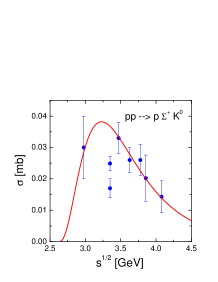
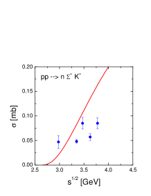
Figure 20: Total cross section of the $pp\to p\Sigma^{+}K^{0}$, $pp\to n\Sigma^{+}K^{+}$ reactions: solid line calculated with eq. (47), dots are the experimental data from Ref. expdata

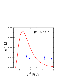
Figure 21: Total cross section of the $pp\to p\Sigma^{0}K^{+}$, $pn\to p\Sigma^{-}K^{+}$ reactions: solid line calculated with eq. (47), dots are the experimental data from Ref. expdata

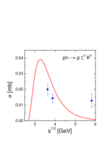
Figure 22: Total cross section of the $pn\to p\Sigma^{0}K^{0}$ reaction: solid line calculated with eq. (47), dots are the experimental data from Ref. expdata

These parameterizations are compared with the experimental data in Figs. 20, 21, 22.

Next we proceed to reactions of the type $NN\to NNK\bar{K}$. Following eff we will use the same isospin-averaged cross sections cas

$$\bar{\sigma}(NN\to NNK\bar{K})=1.5\left(1-\frac{s_{1}}{s}\right)^{3.17}\left(\frac{s_{1}}{s}\right)^{1.96}$$ (48)

with $s_{1}=(2m_{N}+2m_{K})^{2}$ for all possible isospin channels

(54)

Cross sections for processes $NN\to\Delta\Lambda K$ and $NN\to\Delta\Sigma K$ were calculated in Ref. tstl . The cross sections of reactions $pp\to\Delta^{++}\Lambda K^{0}$ and $pp\to\Delta^{++}\Sigma^{-}K^{+}$ are parameterized as follows

$$\sigma(pp\to\Delta^{++}\,\Lambda\,\,K^{0}\,)\!\!\! = \!\!\!6.166\left[\frac{s}{s_{\Delta\Lambda K}}-1\right]^{2.842}\left[\frac{s_{\Delta\Lambda K}}{s}\right]^{1.96}\!\!\!\!,$$

$$\sigma(pp\to\Delta^{++}\Sigma^{-}K^{+})\!\!\! = \!\!\!10.00\left[\frac{s}{s_{\Delta\Sigma K}}-1\right]^{2.874}\left[\frac{s_{\Delta\Sigma K}}{s}\right]^{2.543}\!\!\!\!,$$

where $s_{\Delta\Lambda K}=(m_{\Delta}+m_{\Lambda}+m_{K})^{2}$ and $s_{\Delta\Sigma K}=(m_{\Delta}+m_{\Sigma}+m_{K})^{2}$ . The other reactions channels are related to these two by isospin coefficients $c_{\Lambda}$ and $c_{\Sigma}$

$$\sigma(N_{a}N_{b}\to\Delta_{c}\Lambda K_{d})\!\!\! = \!\!\!c_{\Lambda}\,\sigma(pp\to\Delta^{++}\Lambda K^{0})$$

$$\sigma(N_{a}N_{b}\to\Delta_{c}\Sigma_{d}K_{e})\!\!\! = \!\!\!c_{\Sigma}\,\sigma(pp\to\Delta^{++}\Sigma^{-}K^{+})$$

This coefficients are collected in Table 7.

Table 7: The isospin coefficients in parameterizations of the reactions $NN\to\Delta\Lambda K$ and $NN\to\Delta\Sigma K$ (LABEL:pp2DLk,LABEL:pp2DSk,LABEL:clcs)

reaction	$c_{\Lambda}$	reaction	$c_{\Sigma}$	reaction	$c_{\Sigma}$
$pp\to\Delta^{+}\Lambda K^{+}$	$\frac{1}{3}$	$pp\to\Delta^{+}\,\,\,\Sigma^{0}K^{+}$	$\frac{1}{6}$	$pn\to\Delta^{+}\,\,\,\Sigma^{0}\,K^{0}$	$\frac{1}{6}$
$pn\to\Delta^{+}\Lambda K^{0}$	$\frac{1}{3}$	$pp\to\Delta^{+}\,\,\,\Sigma^{+}K^{0}$	$\frac{1}{3}$	$pn\to\Delta^{0}\,\,\,\,\Sigma^{+}K^{0}$	$\frac{1}{3}$
$pn\to\Delta^{0}\,\Lambda K^{0}$	$\frac{1}{3}$	$pp\to\Delta^{++}\Sigma^{0}K^{0}$	$\frac{1}{2}$	$pn\to\Delta^{++}\Sigma^{-}K^{0}$	$0$
$nn\to\Delta^{0}\,\Lambda K^{0}$	$\frac{1}{3}$	$pp\to\Delta^{0}\,\,\,\,\Sigma^{+}K^{+}$	$0$	$nn\to\Delta^{0}\,\,\,\,\Sigma^{-}K^{+}$	$\frac{1}{3}$
$nn\to\Delta^{-}\Lambda K^{+}$	$1$	$pn\to\Delta^{0}\,\,\,\,\Sigma^{0}K^{+}$	$\frac{1}{6}$	$nn\to\Delta^{-}\,\,\,\Sigma^{0}K^{+}$	$\frac{1}{2}$
		$pn\to\Delta^{+}\,\,\,\Sigma^{-}K^{+}$	$\frac{1}{3}$	$nn\to\Delta^{0}\,\,\,\,\Sigma^{0}\,K^{0}$	$\frac{1}{6}$
		$pn\to\Delta^{-}\,\,\,\Sigma^{+}K^{+}$	$0$	$nn\to\Delta^{-}\,\,\,\Sigma^{+}K^{0}$	$1$
				$nn\to\Delta^{+}\,\,\,\Sigma^{-}K^{0}$	$0$

B.4 Reactions of $\Delta+N$

Reactions $\Delta N\to NYK$ ($Y=\Lambda,\,\Sigma$) are parameterized in tstl in terms of two cross sections

$$\sigma(\Delta^{++}n\to p\Lambda K^{+})=8.337\left[\textstyle\frac{s}{s_{KN\Lambda}}-1\right]^{2.227}\!\!\left[\textstyle\frac{s_{KN\Lambda}}{s}\right]^{2.511}$$

(58)

$$\sigma(\Delta^{-}p\to n\Sigma^{-}K^{+})=52.72\left[\textstyle\frac{s}{s_{KN\Sigma}}-1\right]^{2.799}\!\!\left[\textstyle\frac{s_{KN\Sigma}}{s}\right]^{6.303}$$

(59)

The other reaction channels are related to these two by the isospin coefficients $\bar{c}_{\Lambda}$ and $\bar{c}_{\Sigma}$

$$\sigma(\Delta_{a}N_{b}\to N_{c}\Lambda K_{d})\!\!\! = \!\!\!c_{\Lambda}\,\sigma(\Delta^{++}n\to p\Lambda K^{+})$$

$$\sigma(\Delta_{a}N_{b}\to N_{c}\Sigma_{d}K_{e})\!\!\! = \!\!\!c_{\Sigma}\,\sigma(\Delta^{-}p\to n\Sigma^{-}K^{+})$$

Table 8: The isospin coefficients in parameterizations of the reactions $\Delta N\to NYK$  (58,59,LABEL:bclbcs)

reaction	$\bar{c}_{\Lambda}$	reaction	$\bar{c}_{\Sigma}$	reaction	$\bar{c}_{\Sigma}$
$\Delta^{++}n\to p\Lambda K^{+}$	$1$	$\Delta^{++}p\to p\Sigma^{+}K^{+}$	$0$	$\Delta^{+}n\to p\Sigma^{-}K^{+}$	$\frac{1}{3}$
$\Delta^{+}\,\,\,p\to p\Lambda K^{+}$	$\frac{1}{3}$	$\Delta^{+}\,\,\,p\to p\Sigma^{+}K^{0}$	$\frac{1}{3}$	$\Delta^{0}\,p\to p\Sigma^{-}K^{+}$	$\frac{1}{3}$
$\Delta^{+}\,\,\,n\to p\Lambda K^{0}$	$\frac{1}{3}$	$\Delta^{++}n\to p\Sigma^{+}K^{0}$	$1$	$\Delta^{+}n\to n\Sigma^{0}K^{+}$	$\frac{1}{6}$
$\Delta^{0}\,\,\,\,p\to p\Lambda K^{0}$	$\frac{1}{3}$	$\Delta^{+}\,\,\,p\to p\Sigma^{0}K^{+}$	$\frac{1}{6}$	$\Delta^{0}\,p\to n\Sigma^{0}K^{+}$	$\frac{1}{6}$
$\Delta^{+}\,\,\,n\to n\Lambda K^{+}$	$\frac{1}{3}$	$\Delta^{++}n\to p\Sigma^{0}K^{+}$	$\frac{1}{2}$	$\Delta^{0}\,n\to n\Sigma^{0}K^{0}$	$\frac{1}{6}$
$\Delta^{0}\,\,\,\,p\to n\Lambda K^{+}$	$\frac{1}{3}$	$\Delta^{+}\,\,\,p\to n\Sigma^{+}K^{+}$	$0$	$\Delta^{-}p\to n\Sigma^{0}K^{0}$	$\frac{1}{2}$
$\Delta^{-}\,\,\,p\to n\Lambda K^{0}$	$1$	$\Delta^{++}n\to n\Sigma^{+}K^{+}$	$0$	$\Delta^{0}\,n\to p\Sigma^{-}K^{0}$	$0$
$\Delta^{0}\,\,\,n\to n\Lambda K^{0}$	$\frac{1}{3}$	$\Delta^{+}\,\,\,n\to p\Sigma^{0}K^{0}$	$\frac{1}{6}$	$\Delta^{-}p\to p\Sigma^{-}K^{0}$	$0$
		$\Delta^{0}\,\,\,\,p\to p\Sigma^{0}K^{0}$	$\frac{1}{6}$	$\Delta^{0}\,n\to n\Sigma^{-}K^{+}$	$\frac{1}{3}$
		$\Delta^{+}\,\,\,n\to n\Sigma^{+}K^{0}$	$\frac{1}{3}$	$\Delta^{-}p\to n\Sigma^{-}K^{+}$	$1$
		$\Delta^{0}\,\,\,\,p\to n\Sigma^{+}K^{0}$	$\frac{1}{3}$	$\Delta^{-}n\to n\Sigma^{-}K^{0}$	$0$

For reactions of the type $\Delta N\to NNK\bar{K}$, all channels

(72)

will be taken with the averaged cross section for $NN\to NNK\bar{K}$ eff .

Next, we consider the family of processes $\Delta N\to\Delta YK$ ($Y=\Lambda,\Sigma$). In Ref. tstl the following ten reactions were parameterized:

$$\sigma_{\Delta\Delta}^{(1)} = \sigma(\Delta^{++}p\to\Delta^{++}\Lambda K^{+})$$

$$= 2.704\left[\textstyle\frac{s}{s_{\Delta\Lambda K}}-1\right]^{2.303}\left[\textstyle\frac{s_{\Delta\Lambda K}}{s}\right]^{5.551},$$

$$\sigma_{\Delta\Delta}^{(2)} = \sigma(\Delta^{+}p\to\Delta^{+}\Lambda K^{+})$$

$$= 2.917\left[\textstyle\frac{s}{s_{\Delta\Lambda K}}-1\right]^{2.350}\left[\textstyle\frac{s_{\Delta\Lambda K}}{s}\right]^{6.557},$$

$$\sigma_{\Delta\Delta}^{(3)} = \sigma(\Delta^{+}n\to\Delta^{0}\Lambda K^{+})$$ (73)

$$= 0.312\left[\textstyle\frac{s}{s_{\Delta\Lambda K}}-1\right]^{2.110}\left[\textstyle\frac{s_{\Delta\Lambda K}}{s}\right]^{2.165},$$

$$\sigma_{\Delta\Delta}^{(4)} = \sigma(\Delta^{++}p\to\Delta^{++}\Sigma^{0}K^{+})$$

$$= 10.30\left[\textstyle\frac{s}{s_{\Delta\Sigma K}}-1\right]^{2.748}\left[\textstyle\frac{s_{\Delta\Sigma K}}{s}\right]^{9.321},$$

$$\sigma_{\Delta\Delta}^{(5)} = \sigma(\Delta^{++}n\to\Delta^{++}\Sigma^{-}K^{+})$$

$$= 10.33\left[\textstyle\frac{s}{s_{\Delta\Sigma K}}-1\right]^{2.743}\left[\textstyle\frac{s_{\Delta\Sigma K}}{s}\right]^{8.915},$$

$$\sigma_{\Delta\Delta}^{(6)} = \sigma(\Delta^{+}p\to\Delta^{+}\Sigma^{0}K^{+})$$

$$= 10.62\left[\textstyle\frac{s}{s_{\Delta\Sigma K}}-1\right]^{2.759}\left[\textstyle\frac{s_{\Delta\Sigma K}}{s}\right]^{10.20},$$

$$\sigma_{\Delta\Delta}^{(7)} = \sigma(\Delta^{+}p\to\Delta^{0}\Sigma^{+}K^{+})$$

$$= 0.647\left[\textstyle\frac{s}{s_{\Delta\Sigma K}}-1\right]^{2.830}\left[\textstyle\frac{s_{\Delta\Sigma K}}{s}\right]^{3.862},$$

$$\sigma_{\Delta\Delta}^{(8)} = \sigma(\Delta^{0}p\to\Delta^{+}\Sigma^{-}K^{+})$$

$$= 2.128\left[\textstyle\frac{s}{s_{\Delta\Sigma K}}-1\right]^{2.843}\left[\textstyle\frac{s_{\Delta\Sigma K}}{s}\right]^{5.986},$$

$$\sigma_{\Delta\Delta}^{(9)} = \sigma(\Delta^{+}n\to\Delta^{+}\Sigma^{-}K^{+})$$

$$= 10.57\left[\textstyle\frac{s}{s_{\Delta\Sigma K}}-1\right]^{2.757}\left[\textstyle\frac{s_{\Delta\Sigma K}}{s}\right]^{10.11},$$

$$\sigma_{\Delta\Delta}^{(10)} = \sigma(\Delta^{+}n\to\Delta^{0}\Sigma^{0}K^{+})$$ (74)

$$= 1.112\left[\textstyle\frac{s}{s_{\Delta\Sigma K}}-1\right]^{2.846}\left[\textstyle\frac{s_{\Delta\Sigma K}}{s}\right]^{5.943}$$

The other isospin channels can be expressed in terms of these ten cross sections as it is given in Table 9.

Table 9: Cross sections of reactions $\Delta N\to\Delta YK$ ($Y=\Lambda,\Sigma$) in terms of cross sections (73,74)

$\Delta N\to\Delta\Lambda K$
reaction	$\sigma$	reaction	$\sigma$	reaction	$\sigma$	reaction	$\sigma$	reaction	$\sigma$
$\Delta^{++}p\to\Delta^{++}\Lambda K^{+}$	$\sigma^{(1)}_{\Delta\Delta}$	$\Delta^{++}n\to\Delta^{++}\Lambda K^{0}$	$\sigma^{(1)}_{\Delta\Delta}$	$\Delta^{++}n\to\Delta^{+}\Lambda K^{+}$	$\frac{4}{3}\sigma^{(3)}_{\Delta\Delta}$	$\Delta^{+}p\to\Delta^{++}\Lambda K^{0}$	$\frac{4}{3}\sigma^{(3)}_{\Delta\Delta}$	$\Delta^{+}p\to\Delta^{+}\Lambda K^{+}$	$\sigma^{(2)}_{\Delta\Delta}$
$\Delta^{+}\,\,\,n\to\Delta^{+}\,\,\,\Lambda K^{0}$	$\sigma^{(2)}_{\Delta\Delta}$	$\Delta^{+}\,\,\,n\to\Delta^{0}\,\,\,\,\Lambda K^{+}$	$\sigma^{(3)}_{\Delta\Delta}$	$\Delta^{0}\,\,\,\,p\to\Delta^{+}\Lambda K^{0}$	$\sigma^{(3)}_{\Delta\Delta}$	$\Delta^{0}\,p\to\Delta^{0}\,\,\,\,\,\Lambda K^{+}$	$\sigma^{(2)}_{\Delta\Delta}$	$\Delta^{0}\,n\to\Delta^{0}\Lambda K^{0}$	$\sigma^{(2)}_{\Delta\Delta}$
$\Delta^{0}\,\,\,\,n\to\Delta^{-}\,\,\,\Lambda K^{+}$	$\frac{4}{3}\sigma^{(3)}_{\Delta\Delta}$	$\Delta^{-}\,\,\,p\to\Delta^{0}\,\,\,\,\Lambda K^{0}$	$\frac{4}{3}\sigma^{(3)}_{\Delta\Delta}$	$\Delta^{-}\,\,\,p\to\Delta^{-}\Lambda K^{+}$	$\sigma^{(1)}_{\Delta\Delta}$	$\Delta^{-}n\to\Delta^{-}\,\,\,\Lambda K^{0}$	$\sigma^{(1)}_{\Delta\Delta}$

$\Delta N\to\Delta\Sigma K$
reaction	$\sigma$	reaction	$\sigma$	reaction	$\sigma$	reaction	$\sigma$	reaction	$\sigma$
$\Delta^{++}p\to\Delta^{++}\Sigma^{0}K^{+}$	$\sigma_{\Delta\Delta}^{(4)}$	$\Delta^{+}p\to\Delta^{++}\Sigma^{0}K^{0}$	$\frac{3}{4}\sigma_{\Delta\Delta}^{(10)}$	$\Delta^{+}n\to\Delta^{0}\Sigma^{0}K^{+}$	$\sigma_{\Delta\Delta}^{(10)}$	$\Delta^{0}p\to\Delta^{-}\Sigma^{+}K^{+}$	$\frac{3}{4}\sigma_{\Delta\Delta}^{(7)}$	$\Delta^{-}p\to\Delta^{+}\Sigma^{-}K^{0}$	$0\,\,\,$
$\Delta^{++}p\to\Delta^{++}\Sigma^{+}K^{0}$	$\sigma_{\Delta\Delta}^{(5)}$	$\Delta^{+}p\to\Delta^{+}\Sigma^{0}K^{+}$	$\sigma_{\Delta\Delta}^{(6)}$	$\Delta^{+}n\to\Delta^{++}\Sigma^{-}K^{0}$	$\frac{3}{4}\sigma_{\Delta\Delta}^{(7)}$	$\Delta^{0}n\to\Delta^{0}\Sigma^{0}K^{0}$	$\sigma_{\Delta\Delta}^{(6)}$	$\Delta^{-}p\to\Delta^{-}\Sigma^{+}K^{0}$	$\sigma_{\Delta\Delta}^{(5)}$
$\Delta^{++}p\to\Delta^{+}\Sigma^{+}K^{+}$	$\frac{3}{4}\sigma_{\Delta\Delta}^{(7)}$	$\Delta^{+}p\to\Delta^{+}\Sigma^{+}K^{0}$	$\sigma_{\Delta\Delta}^{(9)}$	$\Delta^{+}n\to\Delta^{-}\Sigma^{+}K^{+}$	$0\,\,\,$	$\Delta^{0}n\to\Delta^{0}\Sigma^{-}K^{+}$	$\sigma_{\Delta\Delta}^{(9)}$	$\Delta^{-}p\to\Delta^{-}\Sigma^{0}K^{+}$	$\sigma_{\Delta\Delta}^{(4)}$
$\Delta^{++}n\to\Delta^{++}\Sigma^{0}K^{0}$	$\sigma_{\Delta\Delta}^{(4)}$	$\Delta^{+}p\to\Delta^{++}\Sigma^{-}K^{+}$	$\frac{3}{4}\sigma_{\Delta\Delta}^{(8)}$	$\Delta^{0}p\to\Delta^{+}\Sigma^{0}K^{0}$	$\sigma_{\Delta\Delta}^{(10)}$	$\Delta^{0}n\to\Delta^{+}\Sigma^{-}K^{0}$	$\sigma_{\Delta\Delta}^{(7)}$	$\Delta^{-}n\to\Delta^{-}\Sigma^{0}K^{0}$	$\sigma_{\Delta\Delta}^{(4)}$
$\Delta^{++}n\to\Delta^{+}\Sigma^{0}K^{+}$	$\frac{3}{4}\sigma_{\Delta\Delta}^{(10)}$	$\Delta^{+}p\to\Delta^{0}\Sigma^{+}K^{+}$	$\sigma_{\Delta\Delta}^{(7)}$	$\Delta^{0}p\to\Delta^{+}\Sigma^{-}K^{+}$	$\sigma_{\Delta\Delta}^{(8)}$	$\Delta^{0}n\to\Delta^{-}\Sigma^{+}K^{0}$	$\frac{3}{4}\sigma_{\Delta\Delta}^{(8)}$	$\Delta^{-}n\to\Delta^{-}\Sigma^{-}K^{+}$	$\sigma_{\Delta\Delta}^{(5)}$
$\Delta^{++}n\to\Delta^{+}\Sigma^{+}K^{0}$	$\frac{3}{4}\sigma_{\Delta\Delta}^{(8)}$	$\Delta^{+}n\to\Delta^{+}\Sigma^{0}K^{0}$	$\sigma_{\Delta\Delta}^{(6)}$	$\Delta^{0}p\to\Delta^{0}\Sigma^{+}K^{0}$	$\sigma_{\Delta\Delta}^{(9)}$	$\Delta^{0}n\to\Delta^{-}\Sigma^{0}K^{+}$	$\frac{3}{4}\sigma_{\Delta\Delta}^{(10)}$	$\Delta^{-}n\to\Delta^{0}\Sigma^{-}K^{0}$	$\frac{3}{4}\sigma_{\Delta\Delta}^{(7)}$
$\Delta^{++}n\to\Delta^{++}\Sigma^{-}K^{+}$	$\sigma_{\Delta\Delta}^{(5)}$	$\Delta^{+}n\to\Delta^{+}\Sigma^{-}K^{+}$	$\sigma_{\Delta\Delta}^{(9)}$	$\Delta^{0}p\to\Delta^{0}\Sigma^{0}K^{+}$	$\sigma_{\Delta\Delta}^{(6)}$	$\Delta^{-}p\to\Delta^{0}\Sigma^{0}K^{0}$	$\frac{3}{4}\sigma_{\Delta\Delta}^{(10)}$
$\Delta^{++}n\to\Delta^{0}\Sigma^{+}K^{+}$	$0\,\,\,$	$\Delta^{+}n\to\Delta^{0}\Sigma^{+}K^{0}$	$\sigma_{\Delta\Delta}^{(8)}$	$\Delta^{0}p\to\Delta^{++}\Sigma^{-}K^{0}$	$0\,\,\,$	$\Delta^{-}p\to\Delta^{0}\Sigma^{-}K^{+}$	$\frac{3}{4}\sigma_{\Delta\Delta}^{(8)}$

B.5 Reactions $\Delta+\Delta$

Reactions $\Delta\Delta\to\Delta YK$ have small cross sections and thus contribute marginally to $K^{+}$ production. Nevertheless, they are included in the calculation with parameterizations from tstl .

$$\bar{\sigma}^{(1)}_{\Delta\Delta} = \sigma(\Delta^{+}\Delta^{++}\to\Delta^{++}\Lambda K^{+})$$

$$= 1.154\left(\frac{s}{s_{\Delta\Lambda K}}-1\right)^{2.149}\left(\frac{s_{\Delta\Lambda K}}{s}\right)^{7.969},$$

$$\bar{\sigma}^{(2)}_{\Delta\Delta} = \sigma(\Delta^{0}\Delta^{++}\to\Delta^{+}\Lambda K^{+})$$

$$= 0.881\left(\frac{s}{s_{\Delta\Lambda K}}-1\right)^{2.150}\left(\frac{s_{\Delta\Lambda K}}{s}\right)^{7.977},$$

$$\bar{\sigma}^{(3)}_{\Delta\Delta} = \sigma(\Delta^{0}\Delta^{+}\to\Delta^{0}\Lambda K^{+})$$ (75)

$$= 0.291\left(\frac{s}{s_{\Delta\Lambda K}}-1\right)^{2.148}\left(\frac{s_{\Delta\Lambda K}}{s}\right)^{7.934},$$

$$\bar{\sigma}^{(4)}_{\Delta\Delta} = \sigma(\Delta^{++}\Delta^{0}\to\Delta^{++}\Sigma^{-}K^{+})$$

$$= 3.532\left(\frac{s}{s_{\Delta\Sigma K}}-1\right)^{2.953}\left(\frac{s_{\Delta\Sigma K}}{s}\right)^{12.06},$$

$$\bar{\sigma}^{(5)}_{\Delta\Delta} = \sigma(\Delta^{++}\Delta^{0}\to\Delta^{+}\Sigma^{0}K^{+})$$

$$= 2.931\left(\frac{s}{s_{\Delta\Sigma K}}-1\right)^{2.952}\left(\frac{s_{\Delta\Sigma K}}{s}\right)^{12.03},$$

$$\bar{\sigma}^{(6)}_{\Delta\Delta} = \sigma(\Delta^{-}\Delta^{+}\to\Delta^{0}\Sigma^{-}K^{+})$$

$$= 5.861\left(\frac{s}{s_{\Delta\Sigma K}}-1\right)^{2.952}\left(\frac{s_{\Delta\Sigma K}}{s}\right)^{12.04},$$

$$\bar{\sigma}^{(7)}_{\Delta\Delta} = \sigma(\Delta^{-}\Delta^{0}\to\Delta^{-}\Sigma^{-}K^{+})$$ (76)

$$= 7.047\left(\frac{s}{s_{\Delta\Sigma K}}-1\right)^{2.952}\left(\frac{s_{\Delta\Sigma K}}{s}\right)^{12.05},$$

The other isospin channels can be expressed in term of these seven cross sections as it is given in Table 10.

Table 10: Cross sections of reactions $\Delta\Delta\to\Delta YK$ ($Y=\Lambda,\Sigma$) in terms of cross sections (75,76)

$\Delta\Delta\to\Delta\Lambda K$
reaction	$\sigma$	reaction	$\sigma$	reaction	$\sigma$	reaction	$\sigma$	reaction	$\sigma$
$\Delta^{++}\Delta^{+}\to\Delta^{++}\Lambda K^{+}$	$\bar{\sigma}^{(1)}_{\Delta\Delta}$	$\Delta^{++}\Delta^{0}\to\Delta^{++}\Lambda K^{0}$	$0\,\,\,$	$\Delta^{++}\Delta^{0}\to\Delta^{+}\Lambda K^{+}$	$\bar{\sigma}^{(2)}_{\Delta\Delta}$	$\Delta^{+}\,\,\,\,\Delta^{+}\to\Delta^{++}\Lambda K^{0}$	$\frac{1}{3}\bar{\sigma}^{(1)}_{\Delta\Delta}$	$\Delta^{+}\Delta^{+}\to\Delta^{+}\Lambda K^{+}$	$\frac{1}{9}\bar{\sigma}^{(1)}_{\Delta\Delta}$
$\Delta^{+}\,\,\,\Delta^{0}\to\Delta^{+}\,\,\,\Lambda K^{0}$	$\bar{\sigma}^{(3)}_{\Delta\Delta}$	$\Delta^{+}\,\,\,\Delta^{0}\to\Delta^{0}\,\,\,\,\Lambda K^{+}$	$\bar{\sigma}^{(3)}_{\Delta\Delta}$	$\Delta^{++}\Delta^{-}\to\Delta^{+}\Lambda K^{0}$	$0\,\,\,$	$\Delta^{++}\Delta^{-}\to\Delta^{0}\,\,\,\,\,\Lambda K^{+}$	$0\,\,\,$	$\Delta^{0}\,\Delta^{0}\to\Delta^{0}\Lambda K^{0}$	$\frac{1}{9}\bar{\sigma}^{(1)}_{\Delta\Delta}$
$\Delta^{0}\,\,\,\,\Delta^{0}\to\Delta^{-}\,\,\,\Lambda K^{+}$	$\frac{1}{3}\bar{\sigma}^{(1)}_{\Delta\Delta}$	$\Delta^{-}\,\,\,\Delta^{+}\to\Delta^{0}\,\,\,\,\Lambda K^{0}$	$\bar{\sigma}^{(2)}_{\Delta\Delta}$	$\Delta^{-}\,\,\,\Delta^{+}\to\Delta^{-}\Lambda K^{+}$	$0\,\,\,$	$\Delta^{-}\,\,\,\Delta^{0}\to\Delta^{-}\,\,\,\Lambda K^{0}$	$\sigma^{(1)}_{\Delta\Delta}$

$\Delta\Delta\to\Delta\Sigma K$
reaction	$\sigma$	reaction	$\sigma$	reaction	$\sigma$	reaction	$\sigma$
$\Delta^{++}\Delta^{+}\to\Delta^{++}\Sigma^{0}K^{+}$	$\frac{1}{2}\bar{\sigma}_{\Delta\Delta}^{(7)}$	$\Delta^{+}\Delta^{+}\to\Delta^{+}\Sigma^{+}K^{0}$	$\frac{1}{9}\bar{\sigma}_{\Delta\Delta}^{(7)}$	$\Delta^{-}\Delta^{++}\to\Delta^{+}\Sigma^{-}K^{+}$	$\bar{\sigma}_{\Delta\Delta}^{(4)}$	$\Delta^{-}\Delta^{+}\to\Delta^{0}\Sigma^{0}K^{0}$	$\bar{\sigma}_{\Delta\Delta}^{(5)}$
$\Delta^{++}\Delta^{+}\to\Delta^{++}\Sigma^{+}K^{0}$	$\bar{\sigma}_{\Delta\Delta}^{(7)}$	$\Delta^{+}\Delta^{+}\to\Delta^{++}\Sigma^{-}K^{+}$	$\frac{1}{3}\bar{\sigma}_{\Delta\Delta}^{(7)}$	$\Delta^{-}\Delta^{++}\to\Delta^{0}\Sigma^{+}K^{0}$	$\bar{\sigma}_{\Delta\Delta}^{(4)}$	$\Delta^{-}\Delta^{+}\to\Delta^{0}\Sigma^{-}K^{+}$	$\bar{\sigma}_{\Delta\Delta}^{(6)}$
$\Delta^{++}\Delta^{+}\to\Delta^{+}\Sigma^{+}K^{+}$	$0\,\,\,$	$\Delta^{+}\Delta^{+}\to\Delta^{0}\Sigma^{+}K^{+}$	$0\,\,\,$	$\Delta^{-}\Delta^{++}\to\Delta^{0}\Sigma^{0}K^{+}$	$\bar{\sigma}_{\Delta\Delta}^{(4)}$	$\Delta^{-}\Delta^{+}\to\Delta^{+}\Sigma^{-}K^{0}$	$0\,\,\,$
$\Delta^{++}\Delta^{0}\,\to\Delta^{++}\Sigma^{0}K^{0}$	$\bar{\sigma}_{\Delta\Delta}^{(4)}$	$\Delta^{+}\Delta^{0}\,\to\Delta^{+}\Sigma^{0}K^{0}$	$\frac{1}{6}\bar{\sigma}_{\Delta\Delta}^{(6)}$	$\Delta^{-}\Delta^{++}\to\Delta^{++}\Sigma^{-}K^{0}$	$0\,\,\,$	$\Delta^{-}\Delta^{+}\to\Delta^{-}\Sigma^{+}K^{0}$	$\bar{\sigma}_{\Delta\Delta}^{(4)}$
$\Delta^{++}\Delta^{0}\,\to\Delta^{+}\Sigma^{0}K^{+}$	$\bar{\sigma}_{\Delta\Delta}^{(5)}$	$\Delta^{+}\Delta^{0}\,\to\Delta^{+}\Sigma^{-}K^{+}$	$\frac{2}{3}\bar{\sigma}_{\Delta\Delta}^{(5)}$	$\Delta^{-}\Delta^{++}\to\Delta^{-}\Sigma^{+}K^{+}$	$0\,\,\,$	$\Delta^{-}\Delta^{+}\to\Delta^{-}\Sigma^{0}K^{+}$	$\bar{\sigma}_{\Delta\Delta}^{(4)}$
$\Delta^{++}\Delta^{0}\,\to\Delta^{+}\Sigma^{+}K^{0}$	$\bar{\sigma}_{\Delta\Delta}^{(6)}$	$\Delta^{+}\Delta^{0}\,\to\Delta^{0}\Sigma^{+}K^{0}$	$\frac{2}{3}\bar{\sigma}_{\Delta\Delta}^{(5)}$	$\Delta^{0}\,\Delta^{0}\,\,\,\,\,\to\Delta^{0}\Sigma^{0}K^{0}$	$\frac{1}{18}\bar{\sigma}_{\Delta\Delta}^{(7)}$	$\Delta^{-}\Delta^{0}\to\Delta^{-}\Sigma^{0}K^{0}$	$\frac{1}{2}\bar{\sigma}_{\Delta\Delta}^{(7)}$
$\Delta^{++}\Delta^{0}\,\to\Delta^{++}\Sigma^{-}K^{+}$	$\bar{\sigma}_{\Delta\Delta}^{(4)}$	$\Delta^{+}\Delta^{0}\to\Delta^{0}\Sigma^{0}K^{+}$	$\frac{1}{6}\bar{\sigma}_{\Delta\Delta}^{(6)}$	$\Delta^{0}\,\Delta^{0}\,\,\,\,\,\to\Delta^{0}\Sigma^{-}K^{+}$	$\frac{1}{9}\bar{\sigma}_{\Delta\Delta}^{(7)}$	$\Delta^{-}\Delta^{0}\to\Delta^{-}\Sigma^{-}K^{+}$	$\bar{\sigma}_{\Delta\Delta}^{(7)}$
$\Delta^{++}\Delta^{0}\,\to\Delta^{0}\Sigma^{+}K^{+}$	$0\,\,\,$	$\Delta^{+}\Delta^{0}\to\Delta^{++}\Sigma^{-}K^{0}$	$0\,\,\,$	$\Delta^{0}\,\Delta^{0}\,\,\,\,\,\to\Delta^{+}\Sigma^{-}K^{0}$	$0\,\,\,$	$\Delta^{-}\Delta^{0}\to\Delta^{0}\Sigma^{-}K^{0}$	$0\,\,\,$
$\Delta^{+}\,\,\,\Delta^{+}\to\Delta^{++}\Sigma^{0}K^{0}$	$\frac{1}{6}\bar{\sigma}_{\Delta\Delta}^{(7)}$	$\Delta^{+}\Delta^{0}\to\Delta^{-}\Sigma^{+}K^{+}$	$0\,\,\,$	$\Delta^{0}\,\Delta^{0}\,\,\,\,\,\to\Delta^{-}\Sigma^{+}K^{0}$	$\frac{1}{3}\bar{\sigma}_{\Delta\Delta}^{(7)}$	$\Delta^{++}\Delta^{++}\to\Delta^{++}\Sigma^{+}K^{+}$	$0\,\,\,$
$\Delta^{+}\,\,\ \Delta^{+}\to\Delta^{+}\Sigma^{0}K^{+}$	$\frac{1}{18}\bar{\sigma}_{\Delta\Delta}^{(7)}$	$\Delta^{-}\Delta^{++}\to\Delta^{+}\Sigma^{0}K^{0}$	$\bar{\sigma}_{\Delta\Delta}^{(4)}$	$\Delta^{0}\,\Delta^{0}\,\,\,\,\,\to\Delta^{-}\Sigma^{0}K^{+}$	$\frac{1}{6}\bar{\sigma}_{\Delta\Delta}^{(7)}$	$\Delta^{-}\,\,\,\Delta^{-}\to\Delta^{-}\Sigma^{-}K^{0}$	$0\,\,\,$

Another group of reactions are $\Delta\Delta\to NNK\bar{K}$. We use the same parameterization (48) for all isospin channels

(88)

B.6 Reactions of $\pi+\pi$

The source of information about $\pi\pi\to K\bar{K}$ reactions is the inelastic $\pi\pi$ scattering which was intensively studied experimentally exppipi . A characteristic feature of the $\pi\pi$ scattering is very rapid rise of the phase shift and the inelasticity parameter at energies about 1 GeV. Such a strong energy dependence is caused by the $f_{0}$ resonance with a pole around $980-i14$ MeV (cf. Ref. oset ). The inelasticity parameter translated into the cross section of the $\pi^{+}\pi^{-}\to K^{+}K^{-}$ reaction pipikk ; petersen is depicted in Fig. 23.

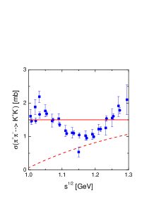
Figure 23: The cross section of the $\pi^{+}\pi^{-}\to K^{+}K^{-}$ reaction: solid line represents parameterization (89), dashed line is calculated as in Refs. mosel ; cas . The experimental points are from pipikk ; petersen

We checked, that the velocity-averaged cross section is reproduced almost exactly if we used a constant for a $\pi\pi\to K\bar{K}$

$$\sigma(\pi^{+}\pi^{-}\to K^{+}K^{-})=\sigma(\pi^{-}\pi^{+}\to K^{0}\bar{K}^{0})=1.6\,\mbox{mb}\,,$$ (89)

shown in Fig. 23 by the solid line. ¿From isospin symmetry, the other $\pi\pi$ channels have cross sections

$$\sigma(\pi^{0}\pi^{0}\to K^{+}K^{-})=\sigma(\pi^{0}\pi^{0}\to K^{0}\bar{K}^{0})$$ (90)

$$\qquad\qquad=\frac{2}{5}\,\sigma(\pi^{+}\pi^{-}\to K^{+}K^{-})=0.64\,\mbox{mb}\,,$$

$$\sigma(\pi^{+}\pi^{0}\to K^{+}\bar{K}^{0})=\sigma(\pi^{-}\pi^{0}\to K^{0}K^{-})$$ (91)

$$\qquad\qquad=\frac{6}{5}\,\sigma(\pi^{+}\pi^{-}\to K^{+}K^{-})=1.92\,\mbox{mb}\,.$$

Note that this implementation is different from the $\pi\pi$ cross sections used in mosel ; cas . The latter is shown in Fig. 23 by the dashed line.

B.7 Reactions of $\rho+\rho$

The cross section for these reactions is not known, because there are no data to which calculations could be compared. It has been calculated in broko as a kaon exchange process. We adopt this result here and parameterize the cross section as

$$\sigma(\rho^{+}\rho^{-}\to K^{+}K^{-})=\sigma(\rho^{+}\rho^{-}\to K^{0}\bar{K}^{0})$$ (92)

$$\qquad\qquad=\frac{1}{32\pi}\,\frac{p^{K}_{cm}}{p^{\rho}_{cm}}\,\exp\left(-\frac{\sqrt{s}-2m_{\rho}}{1\,\mbox{GeV}}\right)\,29.11\,\mbox{mb}\,,$$

where $p^{K}_{cm}(s)$, and $p^{\rho}_{cm}(s)$ are the momenta of kaons and rhos in the centre of mass frame, respectively. The exponential form is chosen such that it reproduces very well the matrix element calculated in broko .

Other $\rho\rho$ channels are determined from isospin symmetry, in analogy to $\pi\pi$ scattering

$$\sigma(\rho^{0}\rho^{0}\to K^{+}K^{-})=\sigma(\rho^{0}\rho^{0}\to K^{0}\bar{K}^{0})$$

$$\qquad\qquad=\frac{2}{5}\,\sigma(\rho^{+}\rho^{-}\to K^{+}K^{-})\,,$$ (93)

$$\sigma(\rho^{+}\rho^{0}\to K^{+}\bar{K}^{0})=\sigma(\rho^{-}\rho^{0}\to K^{0}K^{-})$$

$$\qquad\qquad=\frac{6}{5}\,\sigma(\rho^{+}\rho^{-}\to K^{+}K^{-})\,.$$ (94)

B.8 Reactions of $\pi+\rho$

Production of a $K\bar{K}$ pair in this reaction is suppressed because the $s$-wave component of cross section is forbidden. The reaction is dominated by $\phi$ resonance HSD

$$\sigma(\pi\rho\to\phi\to K\bar{K})=\frac{4\,\pi\,s}{p_{i}^{2}}\,\frac{\Gamma_{\phi\to\pi\rho}\,\left(\frac{k}{k_{0}}\right)^{3}\,\Gamma_{\phi\to K\bar{K}}\,\left(\frac{q}{q_{0}}\right)^{3}}{(s-M^{2}_{\phi})^{2}+s\,\Gamma_{\rm tot}^{2}(\sqrt{s})}\,,$$ (95)

where $p_{i}$ is the momentum of incoming particles in the centre-of-mass system and

$$q_{0}=p_{\rm cm}(M_{\phi}^{2},m_{K},m_{K})\,,\quad q=p_{\rm cm}(s,m_{K},m_{K})\,,$$

$$k_{0}=p_{\rm cm}(M_{\phi}^{2},m_{\pi},m_{\rho})\,,\quad\,\,\,k=p_{\rm cm}(s,m_{\pi},m_{\rho})\,,$$

and the total width is determined from the partial widths

$$\Gamma_{\rm tot}(\sqrt{s})=\Gamma_{\phi\to\pi\rho}\frac{k^{3}}{k_{0}^{3}}+\left(\Gamma_{\phi\to K^{+}K^{-}}+\Gamma_{\phi\to K^{0}\bar{K}^{0}}\right)\frac{q^{3}}{q_{0}^{3}}\,.$$ (96)

The partial widths for decays of $\phi$ into $K^{+}K^{-}$ and $K^{0}_{L}K^{0}_{S}$ are different, but since we keep isospin symmetry in all other reactions throughout this work, we shall use

$$\Gamma_{\phi\to K\bar{K}}=\frac{1}{2}\,\left(\Gamma_{\phi\to K^{+}K^{-}}+\Gamma_{\phi\to K^{0}\bar{K}^{0}}\right)$$ (97)

for all $I=0$ channels.

For the reaction of $\pi\rho$ into $K\bar{K}^{*}$, the leading order diagram in chiral counting is the contact Weinberg-Tomozawa term LK . We calculated the cross section

$$\sigma^{(I)} =\frac{9}{64\pi s}\,\frac{p_{\rm cm}(s,m_{K},m_{K*})}{p_{\rm cm}(s,m_{\pi},m_{\rho})}\,|M^{(I,0)}|^{2}\,\quad I=0,1$$

$$\sigma_{\rm X} =\frac{9}{64\pi s}\,\frac{p_{\rm cm}(s,m_{K},m_{K*})}{p_{\rm cm}(s,m_{\pi},m_{\rho})}\,\Re\Big{(}M^{(0,0)}\,\big{[}M^{(1,0)}\big{]}^{*}\Big{)}\,,$$

using unitarized amplitudes $M^{(I,S)}$, from LK , where $I$ and $S$ are isospin and strangeness quantum numbers indicating a particular reaction channel. The cross sections are shown in Fig. 24.

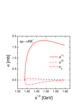
Figure 24: Cross sections for reactions $\pi\rho\to K\bar{K}^{*}$ with given isospin $\sigma^{(0)}$, $\sigma^{(1)}$ and the mixed terms $\sigma_{\rm X}$

We realized that, to a very good approximation, only the $I=1$ component of the cross section effectively contributes and can be replaced by a constant. From combining the involved isospin states we obtain relations

$$\sigma(\rho^{+}\pi^{-}\to K^{+}K^{*-})=\sigma(\rho^{-}\pi^{+}\to K^{0}\bar{K}^{*0})=0.2\,\mbox{mb},$$

$$\sigma(\rho^{-}\pi^{+}\to K^{+}K^{*-})=\sigma(\rho^{+}\pi^{-}\to K^{0}\bar{K}^{*0})=0.2\,\mbox{mb},$$

$$\sigma(\rho^{0}\pi^{0}\to K^{+}K^{*-})=\sigma(\rho^{0}\pi^{0}\to K^{0}\bar{K}^{*0})=0$$

$$\sigma(\rho^{+}\pi^{0}\to K^{+}\bar{K}^{*0})=\sigma(\rho^{0}\pi^{0}\to K^{0}\bar{K}^{*0})=0.4\,\mbox{mb},$$

$$\sigma(\rho^{0}\pi^{+}\to K^{+}\bar{K}^{*0})=\sigma(\rho^{0}\pi^{-}\to K^{0}K^{*-})=0.4\,\mbox{mb}\,.$$

B.9 Decays of $K^{*}$

Kaons can be also produced in decays of $K^{*}$. The decay rate is simply given by $\Gamma_{K^{*}}\rho_{K^{*}}$ where $\Gamma_{K^{*}}=50.8\,\mbox{MeV}$ is the width and $\rho_{K^{*}}$ the density. Individual channels must be multiplied by appropriate Clebsch-Gordan coefficients. These are

$$\begin{array}[]{lll}K^{*+}\to K^{+}\pi^{0}\,,&K^{*0}\to K^{0}\pi^{0}&\to\frac{1}{3}\\ K^{*+}\to K^{0}\pi^{+}\,,&K^{*0}\to K^{+}\pi^{-}&\to\frac{2}{3}\end{array}$$ (101)

The inverse reaction destroys kaons. The cross section is derived as DanBer

$$\sigma(K\pi\to K^{*})=\frac{\pi\,\Gamma_{K^{*}}\,A_{K^{*}}}{2\,p^{2}_{\rm cm}(m_{K^{*}}^{2},m_{\pi},m_{K})}\,,$$ (102)

where

$$A_{K^{*}}(\sqrt{s})=\frac{4\,m_{K^{*}}^{2}\Gamma_{K^{*}}}{(s-m_{K^{*}}^{2})^{2}+m_{K^{*}}^{2}\Gamma_{K^{*}}^{2}}\,.$$ (103)

B.10 Reactions of $Y+\pi$

These reactions produce kaon and a cascade. The cross sections are unknown, so we just use a parameterization

$$\sigma=C\,\frac{p_{\rm cm}(s,m_{\Xi},m_{K})}{p_{\rm cm}(s,m_{Y},m_{\pi})}\,10\,\mbox{mb}\,,$$

where the constant $C$ results from the Clebsch-Gordon coefficients of isospin adding. In the following we just list the parameterizations and the corresponding constants $C$:

$$\begin{array}[]{lllc}\Lambda\pi^{+}\to K^{+}\Xi^{0}\,,&\Lambda\pi^{-}\to K^{0}\Xi^{-}&\to&1\\ \Lambda\pi^{0}\to K^{+}\Xi^{-}\,,&\Lambda\pi^{0}\to K^{0}\Xi^{0}&\to&\frac{1}{2}\end{array}$$ (106)

$$\begin{array}[]{lllc}\Sigma^{+}\pi^{0}\,\to K^{+}\Xi^{0}\,,&\Sigma^{-}\pi^{0}\,\to K^{0}\Xi^{-}&\to&\frac{1}{2}\\ \Sigma^{+}\pi^{-}\to K^{+}\Xi^{-}\,,&\Sigma^{-}\pi^{+}\to K^{0}\Xi^{0}&\to&\frac{5}{12}\\ \Sigma^{0}\,\pi^{+}\to K^{+}\Xi^{0}\,,&\Sigma^{0}\,\pi^{-}\to K^{0}\Xi^{-}&\to&\frac{1}{2}\\ \Sigma^{0}\,\pi^{0}\,\to K^{+}\Xi^{-}\,,&\Sigma^{0}\,\pi^{0}\,\to K^{0}\Xi^{0}&\to&\frac{1}{3}\\ \Sigma^{-}\pi^{+}\to K^{+}\Xi^{-}\,,&\Sigma^{+}\pi^{-}\to K^{0}\Xi^{0}&\to&\frac{5}{12}\end{array}$$ (112)

B.11 Total cross sections of $KN$ reactions

These parameterizations are taken from casibi .

$$\sigma_{K^{+}p}=\begin{cases}12.4&:\quad p_{K}\leq 0.78\\ 1.09+14.5p_{K}&:\quad 0.78<p_{K}\leq 1.17\\ 18.64-0.5p_{K}&:\quad 1.17<p_{K}\leq 2.92\end{cases}$$ (113)

$$\sigma_{K^{+}n}=\begin{cases}15.5&:\quad p_{K}\leq 0.78\\ 4.19+14.5p_{K}&:\quad 0.78<p_{K}\leq 1.1\\ 22.78-2.4p_{K}&:\quad 1.1<p_{K}\leq 2.3\end{cases}$$ (114)

where $p_{K}$ is kaon momentum in the lab frame. In Fig. 25 we illustrate the quality of the paremeterization (113) .

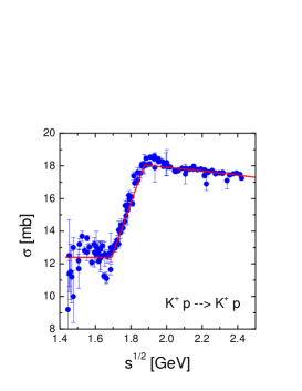
Figure 25: The total $K^{+}p$ cross section as given by (113) in comparison with the experimental data from expdata

Appendix C Feed-down from resonance decays

We list in Table 11 the average numbers of pions which are obtained by decays of individual resonances.

Table 11: List of resonances decaying into pions together with the average numbers of pion species produced by their decays.

	$\langle\pi^{+}\rangle_{R}$	$\langle\pi^{-}\rangle_{R}$		$\langle\pi^{+}\rangle_{R}$	$\langle\pi^{-}\rangle_{R}$
$\eta$	0.28	0.28	$N^{0}(1440)$	0.175	0.725
$\rho^{+}$	1	0	$\bar{N}^{+}(1440)$	0.175	0.725
$\rho^{0}$	1	1	$\bar{N}^{0}(1440)$	0.725	0.175
$\rho^{-}$	0	1	$K^{*+}$	2/3	0
$\omega$	0.91	0.91	$K^{*0}$	0	2/3
$\Delta^{++}$	1	0	$K^{-}$	0	2/3
$\Delta^{+}$	1/3	0	$\bar{K}^{*0}$	2/3	0
$\Delta^{0}$	0	1/3	$\Lambda(1405)$	1/3	1/3
$\Delta^{-}$	0	1	$\Lambda(1520)$	0.217	0.217
$\bar{\Delta}^{++}$	0	1	$\Sigma^{+}(1385)$	0.94	0
$\bar{\Delta}^{+}$	0	1/3	$\Sigma^{0}(1385)$	0.06	0.06
$\bar{\Delta}^{0}$	1/3	0	$\Sigma^{-}(1385)$	0	0.94
$\bar{\Delta}^{-}$	1	0	$\Xi^{-}$	0	1
$N^{+}(1440)$	0.725	0.175	$\Omega$	0	0.322

Resonances which feed-down into kaon, $\Lambda$ and $\Sigma$ production are listed in Table 12.

Table 12: List of resonances decaying into kaons, lambdas or sigmas together with average numbers of decay products.

	$\langle K^{+}\rangle_{R}$	$\langle K^{-}\rangle_{R}$	$\langle\Lambda\rangle_{R}$	$\langle\Sigma^{+}\rangle_{R}$	$\langle\Sigma^{-}\rangle_{R}$
$K^{*+}$	1/3
$K^{*0}$	2/3
$K^{*-}$		1/3
$\bar{K}^{*0}$		2/3
$\Sigma^{0}$			1
$\Lambda(1405)$			1/3	1/3	1/3
$\Lambda(1520)$			0.11	0.143	0.143
$\Sigma^{+}(1385)$			0.94	0.06
$\Sigma^{0}(1385)$			0.88	0.06	0.06
$\Sigma^{-}(1385)$			0.94		0.06
$\Xi^{0}$			1
$\Xi^{-}$			1
$\Omega$		0.678	1

Appendix D Strangeness content of the initial state

D.1 Strangeness multiplicity in $NN$ collisions

Strange particles are also produced in the initial nucleon-nucleon interactions. We shall assume that their initial multiplicities are given by production of kaons in $NN$ reactions in vacuum. Since in our approach kaon production is calculated explicitly and species with $S<0$ are populated statistically, we will only need input on primordial $K^{+}$ production. Data on kaon multiplicities in $pp$ collisions were summarized in grs . In order to obtain the average multiplicity in nucleon-nucleon collisions, we also need multiplicities in $nn$ and $pn$ collisions. It was observed that in $NN$ collisions multiplicity of charged kaons does not depend on isospin of the projectile/target and we can represent $\langle K^{+}\rangle_{NN}$ with $\langle K^{+}\rangle_{pp}$ ondrej ; na49a10

$$\langle K^{+}\rangle_{NN}=\langle K^{+}\rangle_{pp}=\langle K^{+}\rangle_{nn}=\langle K^{+}\rangle_{pn}\,.$$ (115)

D.2 Density from multiplicity

What we actually need for the simulation is the density, not the multiplicity. We will estimate the former by equating

$$\frac{\rho_{K^{+}}}{\rho_{h^{-}}}=\frac{\langle K^{+}\rangle_{NN}}{\langle h^{-}\rangle_{NN}}$$ (116)

Data on multiplicity of negatively charged hadrons from $NN$ interactions were collected by Gaździcki and Röhrich in grns . They collected $h^{-}$ yields from $pp$ and $pn$ collisions at different energies and estimated them for $nn$ collisions. The primordial yield (per nucleon-nucleon pair) for nucleus-nucleus collisions is then obtained as grns

$$\langle h^{-}\rangle_{NN}=\left(\frac{Z}{A}\right)^{2}\langle h^{-}\rangle_{pp}\\ +2\frac{Z}{A}\left(1-\frac{Z}{A}\right)\langle h^{-}\rangle_{pn}+\left(1-\frac{Z}{A}\right)^{2}\langle h^{-}\rangle_{nn}\,.$$ (117)

This relation is formulated for nuclei with atomic number $Z$ which contain $A$ nucleons.

The values for $h^{-}$ yields are not measured at all energies we need. Thus we use data collected in grs ; grns and linearly interpolate as a function of $\sqrt{s}$. The compilation is displayed in Table 13.

Table 13: Multiplicities of negative hadrons in $pp$, $pn$, and $nn$ collisions interpolated from data compiled in grs ; grns . The averaged values for nucleon-nucleon collisions are calculated according to eq. (117).

	$\langle h^{-}\rangle_{pp}$	$\langle h^{-}\rangle_{pn}$	$\langle h^{-}\rangle_{nn}$	$\langle h^{-}\rangle_{NN}$
Au+Au @ 11.6 AGeV	0.697	0.900	1.390	1.044
Pb+Pb @ 30 AGeV	1.265	1.728	1.965	1.741
Pb+Pb @ 40 AGeV	1.482	1.899	2.182	1.937
Pb+Pb @ 80 AGeV	2.025	2.434	2.725	2.477
Pb+Pb @ 158 AGeV	2.611	3.058	3.311	3.081

The resulting ratios $\langle K^{+}\rangle_{NN}/\langle h^{-}\rangle_{NN}$ are listed in Table 2.

D.3 Composition of multiplicity data and feed-down

The major part of the $h^{-}$ multiplicity are pions, a smaller fraction comes from negative kaons. Very small contribution is due to antiprotons. There is feed-down from resonance decays mainly into pion multiplicity. Feed-down to antiprotons is neglected because antibaryons are populated scarcely in general at these energies. Feed-down to $K^{-}$ and $\bar{K}^{0}$ from $K^{*}$ is taken into account.

This is implemented by using the effective densities of pions, kaons and antiprotons when determining the $h^{-}$ density at the left-hand-side of eq. (116)

$$\rho_{h^{-}}=\rho_{\tilde{\pi}^{-}}+\rho_{\tilde{K}^{-}}+\rho_{\bar{p}}\,.$$ (118)

The effective densities, denoted by tildes over subscripts, include the actual densities and pions (kaons) which can be produced by decays of all resonances in the system. These additions are calculated according to the same prescription as the feed-down in final state, see Section II.5 and Appendix C. By using the same strategy we keep the simulation internally consistent.

D.4 Algorithm to obtain the initial state

Technically, the initial state is obtained iteratively:

1. Set densities of all strange particles to zero. Set temperature and chemical potential to some “reasonable” value.

2. Determine energy density and $I_{3}$ density contributions stored in kaons, $\varepsilon_{K}$ and $\rho_{3K}$, respectively. This is done by first determining phase space occupancies $\gamma_{j}$ via

   $$\gamma_{j}=\frac{2\,\pi^{2}\,\rho_{j}}{\exp\left(\frac{I_{3,j}\,\mu_{3}}{T}\right)\,m_{K}^{2}\,T\,K_{2}\left(\frac{m_{K}}{T}\right)}\,,$$ (119)

   where $j=K^{+},\,K^{0}$. Then

   $$\varepsilon_{K}=\frac{1}{2\pi^{2}}\,m_{K}^{2}\,T^{2}\,\left\{\frac{m_{K}}{T}K_{1}\left(\frac{m_{K}}{T}\right)+3K_{2}\left(\frac{m_{K}}{T}\right)\right\}\\ \times\left(\gamma_{K^{+}}\,\exp(\mu_{3}/2T)+\gamma_{K^{0}}\,\exp(-\mu_{3}/2T)\right)\,,$$ (120)

   and

   $$\rho_{3K}=\frac{1}{2}(\rho_{K^{+}}-\rho_{K^{0}})\,.$$ (121)

   Subtract them from the total $\varepsilon$ and $\rho_{3}$, i.e., calculate

   $$\tilde{\varepsilon} = \varepsilon-\varepsilon_{K}$$ (122)

   $$\tilde{\rho}_{3} = \rho_{3}-\rho_{3K}$$ (123)

3. Calculate $\rho_{S}=\rho_{K^{+}}+\rho_{K^{0}}$.

4. ¿From the new $\tilde{\varepsilon},\,\rho_{B},\,\tilde{\rho}_{3},\,\rho_{S}$ calculate temperature, chemical potentials and the suppression factor $\gamma_{S}$.

5. From $T,\,\mu_{B},\,\mu_{3},\,\gamma_{S}$ calculate $\rho_{\tilde{\pi}^{-}}+\rho_{\tilde{K}^{-}}+\rho_{\bar{p}}$. This also includes resonance feed-down to pions and kaons according to the given temperature and chemical potentials.

6. Get $K^{+}$ density as

   $$\rho_{K^{+}}=\frac{\langle K^{+}\rangle_{NN}}{\langle h^{-}\rangle_{NN}}\,(\rho_{\tilde{\pi}^{-}}(T,\mu_{B},\mu_{3},\gamma_{S})\\ +\rho_{\bar{p}}(T,\mu_{B},\mu_{3},\gamma_{S})+\rho_{\tilde{K}^{-}}(T,\mu_{B},\mu_{3},\gamma_{S}))$$ (124)

7. Determine

   $$\rho_{K^{0}}=\rho_{K^{+}}\,\exp(-\mu_{3}/T)$$ (125)

8. Calculate again $\rho_{S}=\rho_{K^{+}}+\rho_{K^{0}}$.

9. If the obtained $\rho_{S}$ differs from that determined in step 3, go to step 2. If they agree, the routine has converged.

References

- (1) C. Alt et al. [NA49 Collaboration], J. Phys. G 30, S119 (2004).
- (2) S.V. Afanasiev et al. [NA49 Collaboration], Phys. Rev. C 66, 054902 (2002).
- (3) J. Cleymans, H. Oeschler, K. Redlich and S. Wheaton, Phys. Lett. B 615, 50 (2005).
- (4) E.L. Bratkovskaya et al., Phys. Rev. C 69, 054907 (2004).
- (5) M. Wagner, A. B. Larionov, U. Mosel, Phys. Rev. C 71, 034910 (2005).
- (6) Yu.B. Ivanov, V.N. Russkikh, V.D. Toneev, nucl-th/0503088.
- (7) J.K. Nayak, J.e. Alam, P. Roy, A.K. Dutt-Mazumder and B. Mohanty, arXiv:nucl-th/0511023.
- (8) M. Gaździcki and M.I. Gorenstein, Acta Physica Polonica B 30, 2705 (1999).
- (9) K. Redlich and A. Tounsi, Eur. Phys. J. C 24, 589 (2002).
- (10) W. Cassing, private communication.
- (11) I. G. Bearden et al. [BRAHMS Collaboration], Phys. Rev. Lett. 93, 102301 (2005).
- (12) F. Rami et al. [FOPI Collaboration], Phys. Rev. Lett. 84, 1120 (2000).
- (13) H.W. Barz, B.L. Friman, J. Knoll, H. Schulz, Nucl. Phys. A 484, 661 (1988).
- (14) H.W. Barz, B.L. Friman, J. Knoll, H. Schulz, Nucl. Phys. A 519, 831 (1990).
- (15) G.E. Brown, C.M. Ko, Z.G. Wu, L.H. Xia, Phys. Rev. C 43, 1881 (1991).
- (16) F. Becattini, M. Gaździcki, A. Keränen, J. Manninen, R. Stock, Phys. Rev. C 69, 024905 (2004); F. Becattini, private communications.
- (17) M. A. Lisa, S. Pratt, R. Soltz and U.A. Wiedemann, Ann. Rev. Nucl. Part. Sci. 55, 357 (2005).
- (18) C.M. Ko and L. Xia, Phys. Rev. C 38, 179 (1988).
- (19) F. Antinori et al. [NA57 Collaboration], J. Phys. G 30, 823 (2004).
- (20) J. P. Bondorf, S. I. A. Garpman and J. Zimányi, Nucl. Phys. A 296, 320 (1978).
- (21) B. Tomášik and U.A. Wiedemann, Phys. Rev. C 68, 034905 (2003).
- (22) S. Albergo et al., Phys. Rev. Lett. 88, 062301 (2003).
- (23) S. Ahmad et al., Phys. Lett. B 382, 35 (1996).
- (24) L. Ahle et al. [E802 Collaboration], Phys. Rev. C 60, 064901 (1999).
- (25) B. B. Back et al., [E917 Collaboration], Phys. Rev. Lett. 87, 242301 (2001).
- (26) F. Becattini, J. Cleymans, A. Keränen, E. Suhonen, K. Redlich, Phys. Rev. C 64, 024901 (2001).
- (27) S. Katz, talk at the conference Quark Matter 2005, Aug.4-9, 2005, Budapest, Hungary; private communication.
- (28) G. Agakichiev et al. [CERES/NA45 collaboration], Phys. Lett. B 422, 405 (1998).
- (29) S. Damjanovic and K. Filimonov [CERES/NA45 Collaboration], Pramana 60, 1067 (2002), [arXiv:nucl-ex/0111009].
- (30) S. Damjanovic for the NA60 collaboration, nucl-ex/0510044.
- (31) J. Cugnon and R.M. Lombard, Nucl. Phys. A422, 635 (1984).
- (32) K. Tsushima, S.W. Huang, A. Faessler, Australian Journal of Physics 50, 35 (1997).
- (33) A. Baldini, V. Flamino, W. G. Moorhead and D. R. O. Morrison, Total Cross Sections of High Energy Particles, Vol. 12 of Landolt-B rnstein, Numerical Data and Functional Relationships in Science and Technology, edited by H. Schopper (Springer-Verlag, Berlin, 1988).
- (34) K. Tsushima, S.W. Huang, A. Faessler, Phys. Lett. B 337, 245 (1994).
- (35) K. Tsushima, S.W. Huang, A. Faessler, J. Phys. G 21, 33 (1995).
- (36) A. Sibirtsev, W. Cassing, C.M. Ko, Z. Phys. A 358, 101 (1997).
- (37) M. Effenberger, Dissertation, Justus-Liebig-Universität Giessen, 1999.
- (38) W. Cassing, E.L. Bratkovskaya, U. Mosel, S. Teis, A. Sibirtsev, Nucl. Phys. A 614, 415 (1997).
- (39) K. Tsushima, A. Sibirtsev, A.W. Thomas, G.Q. Li, Phys. Rev. C 59, 369 (1999).
-
(40)
C. D. Froggatt and J. L. Petersen,
Nucl. Phys. B 129, 89 (1977);
D. H. Cohen et al., Phys. Rev. D 22, 2595 (1980);
A. D. Martin and E. N. Ozmutlu, Nucl. Phys. B 158, 520 (1979);
S. J. Lindenbaum and R. S. Longacre, Phys. Lett. B 274, 492 (1992). - (41) J.A. Oller, E. Oset, and J.R. Peláez, Phys. Rev. D 59, 074001 (1999).
- (42) G. Grayer et al., in International Conference on scattering and associated topics, Tallahassee, 1973 (P.K. Williams and V. Hagopian eds.), AIP Conf. Proc. 13, New York, 1973, p. 117.
- (43) J.L. Petersen, “The interaction”, CERN Yellow Report CERN 77-04, Geneva, 1977.
- (44) M. Wagner, A.B. Larionov, and U. Mosel, Phys. Rev. C 71, 034910 (2005).
- (45) W. Cassing, E.L. Bratkovskaya, Phys. Rep. 308, 65 (1999).
- (46) M.F.M. Lutz and E.E. Kolomeitsev, Nucl. Phys. A 730, 392 (2004).
- (47) P. Danielewicz, G.F. Bertsch, Nucl. Phys. A 533, 712 (1991).
- (48) A. Sibirtsev, W. Cassing, Nucl. Phys. A 641, 476 (1998).
- (49) M. Gaździcki and D. Röhrich, Z. Phys. C 71 (1996) 55.
-
(50)
O. Chvála, Eur. Phys. J. C direct,
DOI 10.1140/epjcd/s2004-03-1704-3. - (51) The NA49 Collaboration, Addendum 10 to proposal CERN/SPSC/P264, CERN/SPSC 2002-008.
- (52) M. Gaździcki and D. Röhrich, Z. Phys. C 65 (1995) 215.