An analytic, parameter-free (up to overall scale factors) solution of the Bohr Hamiltonian involving axially symmetric quadrupole and octupole deformations, as well as an infinite well potential, is obtained, after separating variables in a way reminiscent of the Variable Moment of Inertia (VMI) concept. Normalized spectra and $B(EL)$ ratios are found to agree with experimental data for ²²⁶Ra and ²²⁶Th, the nuclei known to lie closest to the border between octupole deformation and octupole vibrations in the light actinide region.

1. Introduction

Critical point symmetries [1, 2] are attracting recently considerable interest, since they provide parameter-independent (up to overall scale factors) predictions supported by experiment [3, 4, 5, 6]. The E(5) [1] and X(5) [2] critical point symmetries have been obtained from the Bohr Hamiltonian [7] after separating variables in different ways and using an infinite square well potential in the $\beta$ (quadrupole) variable, the latter corresponding to the critical point of the transition from quadrupole vibrations [U(5)] to axial quadrupole deformation [SU(3)] [2]. A systematic study of phase transitions in nuclear collective models has been given in [8, 9, 10].

In the present work a solution of the Bohr Hamiltonian aiming at the description of the transition from axial octupole deformation to octupole vibrations in the light actinides [11] is worked out. In the spirit of E(5) and X(5) the solution involves an infinite square well potential in the deformation variable and leads to parameter-free (up to overal scale factors) predictions for spectra and $B(EL)$ transition rates. Both (axially symmetric) quadrupole and octupole deformations are taken into account, in order to describe low-lying negative parity states related to octupole deformation, known to occur in the light actinides [11]. Separation of variables is achieved in a novel way, reminiscent of the Variable Moment of Inertia (VMI) concept [12]. The parameter-free predictions of the model turn out to be in good agreement with experimental data for ²²⁶Ra [13] and ²²⁶Th [14], the nuclei known [15, 16] to lie closest to the transition from octupole deformation to octupole vibrations in this region.

In Section 2 of the present work the solution is worked out. Numerical results are given and compared to experimental data in Section 3, while Section 4 contains discussion of the present results and plans for further work.

2. The model

When only axially symmetric quadrupole ($\beta_{2}$) and octupole ($\beta_{3}$) deformations are taken into account, the Hamiltonian reads [17, 18]

$$H=-\sum_{\lambda=2,3}{\hbar^{2}\over 2B_{\lambda}}{1\over\beta_{\lambda}^{3}}{\partial\over\partial\beta_{\lambda}}\beta_{\lambda}^{3}{\partial\over\partial\beta_{\lambda}}+{\hbar^{2}\hat{L^{2}}\over 6(B_{2}\beta_{2}^{2}+2B_{3}\beta_{3}^{2})}+V(\beta_{2},\beta_{3})$$ (1)

where $B_{2}$, $B_{3}$ are the mass parameters.

One then seeks solutions of the Schrödinger equation of the form [17]

$$\Phi^{\pm}_{L}(\beta_{2},\beta_{3},\theta)=(\beta_{2}\beta_{3})^{-3/2}\Psi^{\pm}_{L}(\beta_{2},\beta_{3})|LM0,\pm\rangle,$$ (2)

where $M$ is the angular momentum projection onto the laboratory-fixed $\hat{z}$-axis, $K=0$ is the projection onto the body-fixed $\hat{z}^{\prime}$-axis, and the functions $|LM0,+\rangle$ and $|LM0,-\rangle$ transform according to the irreducible representations (irreps) A and B₁ of the group D₂ respectively [17, 18], their explicit form being given in [16, 19].

Introducing [17, 18]

$$\tilde{\beta}_{2}=\beta_{2}\sqrt{B_{2}\over B},\quad\tilde{\beta}_{3}=\beta_{3}\sqrt{B_{3}\over B},\quad B={B_{2}+B_{3}\over 2},$$ (3)

reduced energies $\epsilon=(2B/\hbar^{2})E$ and reduced potentials $u=(2B/\hbar^{2})V$ [1, 2], as well as polar coordinates (with $0\leq\tilde{\beta}<\infty$ and $-\pi/2\leq\phi\leq\pi/2$) [17, 18]

$$\tilde{\beta}_{2}=\tilde{\beta}\cos\phi,\quad\tilde{\beta}_{3}=\tilde{\beta}\sin\phi,\quad\tilde{\beta}=\sqrt{\tilde{\beta}_{2}^{2}+\tilde{\beta}_{3}^{2}},$$ (4)

the Schrödinger equation takes the form [16]

$$\left[-{\partial^{2}\over\partial\tilde{\beta}^{2}}-{1\over\tilde{\beta}}{\partial\over\partial\tilde{\beta}}+{L(L+1)\over 3\tilde{\beta}^{2}(1+\sin^{2}\phi)}-{1\over\tilde{\beta}^{2}}{\partial^{2}\over\partial\phi^{2}}+u(\tilde{\beta},\phi)+{3\over\tilde{\beta}^{2}\sin^{2}2\phi}-\epsilon_{L}\right]\Psi_{L}^{\pm}(\tilde{\beta},\phi)=0.$$ (5)

Separation of variables in Eq. (5) can be achieved by assuming the potential to be of the form [17, 20] $u(\tilde{\beta},\phi)=u(\tilde{\beta})+u(\phi)/\tilde{\beta}^{2}$, leading to

$$\tilde{\beta}^{2}\left(-{\partial^{2}\over\partial\tilde{\beta}^{2}}-{1\over\tilde{\beta}}{\partial\over\partial\tilde{\beta}}+u(\tilde{\beta})-\epsilon_{\tilde{\beta}}(L)\right)\psi^{\pm}_{L}(\tilde{\beta})=-\nu^{2}\psi^{\pm}_{L}(\tilde{\beta}),$$ (6)

$$\left({\partial^{2}\over\partial\phi^{2}}-u(\phi)-u_{L}(\phi)\right)\chi^{\pm}(\phi)=-\nu^{2}\chi^{\pm}(\phi),$$ (7)

where

$$u_{L}(\phi)={3\over\sin^{2}2\phi}+{L(L+1)\over 3(1+\sin^{2}\phi)},$$ (8)

with $\nu^{2}$ being the separation constant and $\Psi^{\pm}_{L}(\tilde{\beta},\phi)=\psi^{\pm}_{L}(\tilde{\beta})\chi^{\pm}(\phi)$, where, however, the $\pm$ indices have become redundant.

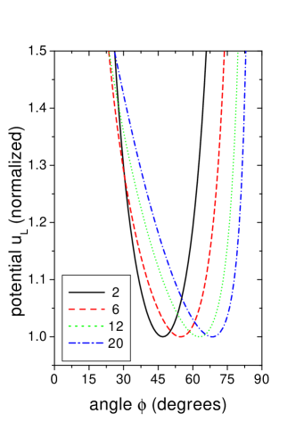
Figure 1: Potential $u_{L}$ [Eq. (8)] for different values of the angular momentum $L$, normalized for each $L$ to its minimum value. See section 2 for further discussion.

The potential $u_{L}(\phi)$ of Eq. (8) is shown in Fig. 1 for several values of $L$, normalized to its minimum value for each $L$. It is clear that in each case the potential has the form of a deep well, possessing an $L$-dependent minimum, denoted by $\phi_{L}$ and determined from the equation

$$u^{\prime}_{L}(\phi)=-{2\over 3}{L(L+1)\sin\phi\cos\phi\over(1+\sin^{2}\phi)^{2}}-{12\cos 2\phi\over\sin^{3}2\phi}=0.$$ (9)

Using standard trigonometric identities and defining $x=\sin^{2}\phi$ and $b=9/(4L(L+1))$ one easily sees that Eq. (9) takes the form

$$x^{4}-2(1+b)x^{3}+(1-3b)x^{2}+b=0,$$ (10)

which turns out to have only one real root in the interval $0\leq x\leq 1$ (imposed by $x=\sin^{2}\phi$).

Given its form, the potential $u_{L}(\phi)$ can be approximated around the minimum by the first terms of the Taylor expansion as

$$u_{L}(\phi)\approx u_{L}(\phi_{L})+{u^{\prime\prime}_{L}(\phi_{L})\over 2}(\phi-\phi_{L})^{2}.$$ (11)

In Eq. (7) one can then omit the potential $u(\phi)$, treating $u_{L}(\phi)$ as an effective potential naturally occuring in the framework of the theory, leading Eq. (7) into the harmonic oscillator form

$$-{\partial^{2}\chi\over\partial\zeta^{2}}+\zeta^{2}\chi=\varepsilon_{L}\chi,$$ (12)

with

$$\zeta^{2}=\sqrt{{u^{\prime\prime}_{L}(\phi_{L})\over 2}}(\phi-\phi_{L})^{2},\qquad\varepsilon_{L}={\nu^{2}-u_{L}(\phi_{L})\over\sqrt{{u^{\prime\prime}_{L}(\phi_{L})\over 2}}}.$$ (13)

Since $\varepsilon_{L}=2n+1$, where $n$ is the number of oscillator quanta, one obtains

$$\nu^{2}=\sqrt{u^{\prime\prime}_{L}(\phi_{L})\over 2}(2n+1)+u_{L}(\phi_{L}).$$ (14)

In what follows we are going to be limited to the case $n=0$.

Returning to Eq. (6), using for $u(\tilde{\beta})$ an infinite well potential ($u(\tilde{\beta})=0$ if $\tilde{\beta}\leq\tilde{\beta}_{W}$; $u(\tilde{\beta})=\infty$ if $\tilde{\beta}>\tilde{\beta}_{W}$), and defining [2] $\epsilon_{\tilde{\beta}}=k_{\tilde{\beta}}^{2}$, $z=\tilde{\beta}k_{\tilde{\beta}}$, one is led to the Bessel equation

$${d^{2}\psi_{\nu}\over dz^{2}}+{1\over z}{d\psi_{\nu}\over dz}+\left[1-{\nu^{2}\over z^{2}}\right]\psi_{\nu}=0.$$ (15)

Then the boundary condition $\psi_{\nu}(\tilde{\beta}_{W})=0$ determines the spectrum

$$\epsilon_{\tilde{\beta},s,\nu}=\epsilon_{\tilde{\beta},s,L}=(k_{s,\nu})^{2},\qquad k_{s,\nu}={x_{s,\nu}\over\tilde{\beta}_{W}},$$ (16)

and the eigenfunctions

$$\psi_{s,\nu}(\tilde{\beta})=\psi_{s,L}(\tilde{\beta})=c_{s,\nu}J_{\nu}(k_{s,\nu}\tilde{\beta}),$$ (17)

where $x_{s,\nu}$ is the $s$th zero of the Bessel function $J_{\nu}(z)$, while $c_{s,\nu}$ are normalization constants, determined from the condition $\int_{0}^{\tilde{\beta}_{W}}|\psi_{s,\nu}(\tilde{\beta})|^{2}\tilde{\beta}d\tilde{\beta}=1$ to be $c_{s,\nu}=\sqrt{2}/J_{\nu+1}(k_{s,\nu})$. The notation has been kept similar to that of Ref. [2].

A few comments are now in place:

a) $L$-dependent potentials, as the one of Eq. (8), are known to occur in nuclear physics in the framework of the optical model potential [21], as well as in the study of quasimolecular resonances, such as ¹²C+¹²C [22].

b) The procedure followed for the determination of $\phi_{L}$ is reminiscent of the Variable Moment of Inertia (VMI) model [12]. In the VMI case the energy is minimized with respect to the moment of inertia for each $L$ separately, resulting in a moment of inertia increasing with $L$. In the present case the effective potential energy $u_{L}$ is minimized with respect to $\phi$ for each $L$ separately, resulting in $\phi_{L}$ values increasing with $L$. As a consequence, in Eq. (8) the denominator of $L(L+1)$, which can be considered roughly as playing the role of a moment of inertia, is also increasing with $L$.

c) In order to separate variables, one can in general assume $u(\beta,\gamma)=u(\beta)+u(\gamma)$, as in the X(5) model [2], or $u(\beta,\gamma)=u(\beta)+u(\gamma)/\beta^{2}$, as in Refs. [17, 20]. In the former case the separation is approximate, since a $\beta^{2}$ term is involved in the $\gamma$ equation, replaced by its average value, but no extra parameter is introduced in the $\beta$-equation by the separation. In the latter case, the separation is exact, but (at least) one extra parameter appears in the $\beta$-equation, coming in from the $\gamma$-equation through the separation constant. In the present model this disadvantage of the latter case is avoided through the VMI-like procedure adapted.

d) For each $L$ the specific value of the variable $\phi$, which decides the relative presence of the quadrupole and octupole deformations, is determined in Eq. (7) by the effective potential $u_{L}(\phi)$, which has a rigid shape, as seen in Fig. 1, while the potential $u(\phi)$ plays no role.

The calculation of $B(EL)$ transition rates proceeds as in Ref. [16] and need not be repeated here.

3. Numerical results and comparison to experiment

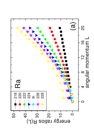
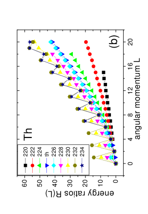
Figure 2: (a) Experimental energy ratios $R(L)=E(L)/E(2_{1}^{+})$ for ²¹⁸Ra [14, 23], ²²⁰Ra [14], and ^222-228Ra [13], compared to theoretical predictions. (b) Same for ^220-228Th [14], ²³⁰Th [13], ²³²Th [13, 14], and ²³⁴Th [13].

The parameter-free predictions of the model for the lowest bands are given in Table 1, together with the experimental spectra of ²²⁶Ra [13] and ²²⁶Th [14], which are known to lie near the border between the regions of octupole deformation and octupole vibrations [15, 16], as also seen in Figs. 2(a) and 2(b), where the experimental spectra of ^218-228Ra and ^220-234Th are included. In both figures the region below the theoretical predictions corresponds to octupole deformation, characterized by minimal odd-even staggering rapidly decreasing and disappearing with increasing $L$, while the region above the theoretical predictions corresponds to octupole vibrations, characterized by large odd-even staggering decreasing very slowly with increasing $L$. As seen in Table 1, in the case of ²²⁶Ra and ²²⁶Th the odd-even staggering is non-negligible only for the lowest four odd levels, the agreement between theory and experiment being very good for the even levels, as well as with the rest of the odd ones. The absence of staggering in the present model is due to the fact that the (infinite) potential wells for $\beta_{3}<0$ and $\beta_{3}>0$ [see Eq. (4)] are separated by an infinite barrier, and not by a finite one, as needed for odd-even staggering to be present [24].

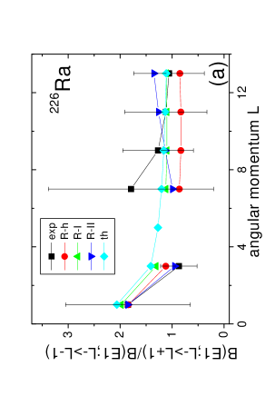
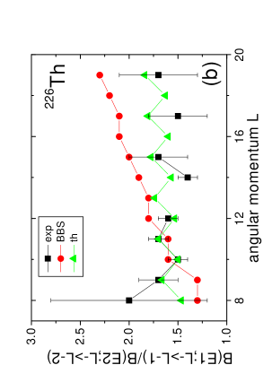
Figure 3: (a) Experimental $B(E1;L\to L+1)$ / $B(E1;L\to L-1)$ ratios [25] of $B(E1)$ values originating from the same level of ²²⁶Ra, compared to three different theoretical predictions from Ref. [27] (labeled as R-h, R-I, R-II), as well as to theoretical predictions of the present model. See section 3 for further discussion. (b) Experimental $B(E1;L\to L-1)$ / $B(E2;L\to L-2)$ ratios (multiplied by $10^{5}$) [15] of $B(E1)$ and $B(E2)$ values originating from the same level of ²²⁶Th, compared to theoretical predictions by Bizzeti and Bizzeti-Sona [15] (labeled as BBS), as well as to predictions of the present model. The ratios corresponding to $L=10$ and 11 have been used for normalization, as in Ref. [15].

Several parameter-free predictions for $B(E1)$, $B(E2)$, and $B(E3)$ transition rates, appropriately normalized, are reported in Table 2. Since the lack of experimental data does not allow for direct comparison to experiment, comparisons to $B(E1)$ branching ratios of ²²⁶Ra [25] and $B(E1)/B(E2)$ ratios for ²²⁶Th [15] are shown in Figs. 3(a) and 3(b) respectively. The theoretical predictions in Fig. 3(a) are compatible with the data within the experimental errors, while in addition they are quite similar to predictions of the Extended Coherent States Model (ECSM) [26] obtained with the lowest order $E1$ operator (R-h), as well as with two different choices of the $E1$ operator including anharmonicities (R-I, R-II) [27]. The theoretical predictions in Fig. 3(b) are also compatible with the data within the experimental errors, lying considerably lower than the predictions of Ref. [15] (BBS).

It is worth remarking that the ground state band spectrum and intraband $B(E2)$s of the present model are quite similar to these of the X(5) model [2] (extensively tabulated in Ref. [28]). Indeed the present model can be considered as an extension of X(5), in which the octupole degree of freedom is taken into account in order to account for the low-lying negative parity bands, while in parallel the $\gamma$ degree of freedom is left out in order to keep the problem tractable. One important difference between the two models is related to the (normalized) position of the $0_{2}^{+}$ state, which is predicted at 5.649 by the X(5) model [2], but at 12.569 by the present model. This implies that while searching for X(5)-like nuclei in the light actinide region, one should expect the $0_{2}^{+}$ state to occur higher by a factor of two. Indeed the Ra and Th isotopes near $A=226$ exhibit high-lying $0_{2}^{+}$ states [13, 14].

It should also be noticed that the predictions of the present parameter-independent model are very similar to those of the one-parameter ($\phi_{0}$) Analytic Quadrupole Octupole Axially symmetric (AQOA) model [16], in which best agreement to experiment is obtained for $\phi_{0}=56^{\rm o}$ in the case of ²²⁶Ra, and for $\phi_{0}=60^{\rm o}$ in the case of ²²⁶Th. These values of $\phi_{0}$ are understandable, when compared to the $\phi_{L}$ values shown in Table 1.

4. Discussion

A parameter-free (up to overall scale factors) version of an Analytic Quadrupole Octupole Axially symmetric (AQOA) model involving an infinite well potential, suitable for describing the transition from octupole deformation to octupole vibrations in the light actinides, has been constructed, after separating variables in the Bohr Hamiltonian in a way reminiscent of the Variable Moment of Inertia concept. Spectra and $B(EL)$ ratios are shown to be in good agreement with experimental data for ²²⁶Ra and ²²⁶Th, the nuclei supposed to lie closest to the above mentioned border. Application of the model in the $A\approx 150$ region, where octupole deformation is also well established [11], is receiving attention.

Table 1: Spectra of the present model for the ground state band and the associated negative parity band ($s=1$), as well as for the first excited band ($s=2$), together with relevant values of $\phi_{L}$ and experimental data for ²²⁶Ra [13] and ²²⁶Th [14]. Each spectrum is normalized to the energy of its own $2_{1}^{+}$ state. See section 3 for further discussion.

$L^{\pi}$	$\phi_{L}$	th	226Ra	226Th	$L^{\pi}$	$\phi_{L}$	th	226Ra	226Th
$s=1$
$0^{+}$	45.00	0.000	0.000	0.000	$1^{-}$	45.70	0.337	3.747	3.191
$2^{+}$	47.01	1.000	1.000	1.000	$3^{-}$	48.77	1.967	4.749	4.259
$4^{+}$	50.77	3.200	3.127	3.136	$5^{-}$	52.79	4.657	6.603	6.240
$6^{+}$	54.71	6.297	6.155	6.195	$7^{-}$	56.47	8.093	9.264	9.112
$8^{+}$	58.05	10.025	9.891	9.999	$9^{-}$	59.46	12.081	12.677	12.785
$10^{+}$	60.73	14.254	14.185	14.409	$11^{-}$	61.86	16.537	16.743	17.152
$12^{+}$	62.89	18.928	18.931	19.324	$13^{-}$	63.81	21.424	21.388	22.105
$14^{+}$	64.65	24.023	24.061	24.675	$15^{-}$	65.42	26.724	26.536	27.554
$16^{+}$	66.13	29.526	29.523	30.413	$17^{-}$	66.78	32.427	32.126	33.418
$18^{+}$	67.38	35.428	35.300	36.497	$19^{-}$	67.94	38.527	38.099	39.627
$20^{+}$	68.46	41.724	41.375	42.896
$s=2$
$0^{+}$	45.00	12.569	12.186	11.152
$2^{+}$	47.01	14.253
$4^{+}$	50.77	17.871

Table 2: $B(EL;L_{i}\to L_{f})$ values between states of the present model with $s=1$. $B(E2)$s with $L_{i}$ and $L_{f}$ even are normalized to the $2_{1}^{+}\to 0_{1}^{+}$ transition, while $B(E2)$s with $L_{i}$ and $L_{f}$ odd are normalized to the $3_{1}^{-}\to 1_{1}^{-}$ transition. $B(E1)$s are normalized to the $1_{1}^{-}\to 0_{1}^{+}$ transition, while $B(E3)$s are normalized to the $3_{1}^{-}\to 0_{1}^{+}$ transition. See section 3 for further discussion.

$L_{i}^{\pi}$	$L_{f}^{\pi}$	$B(E2)$	$L_{i}^{\pi}$	$L_{f}^{\pi}$	$B(E1)$	$L_{i}^{\pi}$	$L_{f}^{\pi}$	$B(E3)$ $L_{i}^{\pi}$	$L_{f}^{\pi}$	$B(E3)$
$2^{+}$	$0^{+}$	1.000	$1^{-}$	$0^{+}$	1.000	$3^{-}$	$0^{+}$	1.000	$2^{+}$	$1^{-}$	1.793
$4^{+}$	$2^{+}$	1.494	$2^{+}$	$1^{-}$	1.238	$4^{+}$	$1^{-}$	1.358	$3^{-}$	$2^{+}$	1.362
$6^{+}$	$4^{+}$	1.749	$3^{-}$	$2^{+}$	1.389	$5^{-}$	$2^{+}$	1.581	$4^{+}$	$3^{-}$	1.341
$8^{+}$	$6^{+}$	1.944	$4^{+}$	$3^{-}$	1.522	$6^{+}$	$3^{-}$	1.752	$5^{-}$	$4^{+}$	1.369
$10^{+}$	$8^{+}$	2.103	$5^{-}$	$4^{+}$	1.650	$7^{-}$	$4^{+}$	1.896	$6^{+}$	$5^{-}$	1.411
$12^{+}$	$10^{+}$	2.237	$6^{+}$	$5^{-}$	1.775	$8^{+}$	$5^{-}$	2.022	$7^{-}$	$6^{+}$	1.456
$14^{+}$	$12^{+}$	2.350	$7^{-}$	$6^{+}$	1.896	$9^{-}$	$6^{+}$	2.136	$8^{+}$	$7^{-}$	1.500
$16^{+}$	$14^{+}$	2.448	$8^{+}$	$7^{-}$	2.012	$10^{+}$	$7^{-}$	2.238	$9^{-}$	$8^{+}$	1.542
$18^{+}$	$16^{+}$	2.534	$9^{-}$	$8^{+}$	2.123	$11^{-}$	$8^{+}$	2.331	$10^{+}$	$9^{-}$	1.582
$20^{+}$	$18^{+}$	2.611	$10^{+}$	$9^{-}$	2.228	$12^{+}$	$9^{-}$	2.416	$11^{-}$	$10^{+}$	1.620
			$11^{-}$	$10^{+}$	2.328	$13^{-}$	$10^{+}$	2.494	$12^{+}$	$11^{-}$	1.655
$3^{-}$	$1^{-}$	1.000	$12^{+}$	$11^{-}$	2.424	$14^{+}$	$11^{-}$	2.566	$13^{-}$	$12^{+}$	1.689
$5^{-}$	$3^{-}$	1.246	$13^{-}$	$12^{+}$	2.515	$15^{-}$	$12^{+}$	2.632	$14^{+}$	$13^{-}$	1.720
$7^{-}$	$5^{-}$	1.413	$14^{+}$	$13^{-}$	2.602	$16^{+}$	$13^{-}$	2.694	$15^{-}$	$14^{+}$	1.750
$9^{-}$	$7^{-}$	1.547	$15^{-}$	$14^{+}$	2.685	$17^{-}$	$14^{+}$	2.752	$16^{+}$	$15^{-}$	1.777
$11^{-}$	$9^{-}$	1.658	$16^{+}$	$15^{-}$	2.764	$18^{+}$	$15^{-}$	2.806	$17^{-}$	$16^{+}$	1.804
$13^{-}$	$11^{-}$	1.752	$17^{-}$	$16^{+}$	2.840	$19^{-}$	$16^{+}$	2.856	$18^{+}$	$17^{-}$	1.829
$15^{-}$	$13^{-}$	1.832	$18^{+}$	$17^{-}$	2.913	$20^{+}$	$17^{-}$	2.904	$19^{-}$	$18^{+}$	1.852
$17^{-}$	$15^{-}$	1.902	$19^{-}$	$18^{+}$	2.983				$20^{+}$	$19^{-}$	1.875
$19^{-}$	$17^{-}$	1.964	$20^{+}$	$19^{-}$	3.050

References

- [1] F. Iachello, Phys. Rev. Lett. 85 (2000) 3580.
- [2] F. Iachello, Phys. Rev. Lett. 87 (2001) 052502.
- [3] R. F. Casten and N. V. Zamfir, Phys. Rev. Lett. 85 (2000) 3584.
- [4] R. M. Clark, et al., Phys. Rev. C 69 (2004) 064322.
- [5] R. F. Casten and N. V. Zamfir, Phys. Rev. Lett. 87 (2001) 052503.
- [6] R. M. Clark, et al., Phys. Rev. C 68 (2003) 037301.
- [7] A. Bohr, Mat. Fys. Medd. K. Dan. Vidensk. Selsk. 26 (1952) no. 14.
- [8] D. J. Rowe, Nucl. Phys. A 745, 47 (2004).
- [9] P. S. Turner and D. J. Rowe, Nucl. Phys. A 756, 333 (2005).
- [10] G. Rosensteel and D. J. Rowe, Nucl. Phys. A 759, 92 (2005).
- [11] P. A. Butler and W. Nazarewicz, Rev. Mod. Phys. 68 (1996) 349.
- [12] M. A. J. Mariscotti, G. Scharff-Goldhaber, and B. Buck, Phys. Rev. 178 (1969) 1864.
- [13] J. F. C. Cocks, et al., Nucl. Phys. A 645 (1999) 61.
- [14] Nuclear Data Sheets, as of December 2004.
- [15] P. G. Bizzeti and A. M. Bizzeti-Sona, Phys. Rev. C 70 (2004) 064319.
- [16] D. Bonatsos, D. Lenis, N. Minkov, D. Petrellis, and P. Yotov, Phys. Rev. C 71 (2005) 064309.
- [17] A. Ya. Dzyublik and V. Yu. Denisov, Yad. Fiz. 56 (1993) 30 [Phys. At. Nucl. 56 (1993) 303].
- [18] V. Yu. Denisov and A. Ya. Dzyublik, Nucl. Phys. A 589 (1995) 17.
- [19] A. Bohr and B. R. Mottelson, Nuclear Structure, Vol. II, Benjamin, New York, 1975.
- [20] L. Fortunato, Phys. Rev. C 70 (2004) 011302(R).
- [21] H. Fiedelday amd S. A. Sofianos, Z. Phys. A 311 (1983) 339.
- [22] W. Greiner, J. Y. Park, and W. Scheid, Nuclear Molecules, World Scientific, Singapore, 1995.
- [23] N. Schulz, et al., Phys. Rev. Lett. 63 (1989) 2645.
- [24] R. V. Jolos and P. von Brentano, Phys. Rev. C 49 (1994) R2301.
- [25] H. J. Wollersheim, et al., Nucl. Phys. A 556 (1993) 261.
- [26] A. A. Raduta, Recent Res. Devel. Nuclear Phys. 1 (2004) 1.
- [27] A. A. Raduta, D. Ionescu, I. I. Ursu, and A. Faessler, Nucl. Phys. A 720 (2003) 43.
- [28] D. Bonatsos, D. Lenis, N. Minkov, P. P. Raychev and P. A. Terziev, Phys. Rev. C 69 (2004) 014302.