Three-body continuum states on a Lagrange mesh

Abstract

Three-body continuum states are investigated with the hyperspherical method on a Lagrange mesh. The $R$-matrix theory is used to treat the asymptotic behaviour of scattering wave functions. The formalism is developed for neutral as well as for charged systems. We point out some specificities of continuum states in the hyperspherical method. The collision matrix can be determined with a good accuracy by using propagation techniques. The method is applied to the ⁶He (=$\alpha$+n+n) and ⁶Be (=$\alpha$+p+p) systems, as well as to ¹⁴Be (=¹²Be+n+n). For ⁶He, we essentially recover results of the literature. Application to ¹⁴Be suggests the existence of an excited $2^{+}$ state below threshold. The calculated B(E2) value should make this state observable with Coulomb excitation experiments.

I Introduction

Three-body systems present a large variety of interesting features Jo04 ; ZDF93 . The discovery of a halo structure in ⁶He THH85 triggered many experimental and theoretical works on exotic nuclei, such as ⁶He, ¹¹Li or ¹⁴Be. The bound-state spectroscopy of Borromean systems is now relatively well known. On the experimental side, current intensities of radioactive beams are high enough for precise measurements of spectroscopic properties, such as energies, r.m.s. radii on quadrupole moments. On the theoretical side, several methods have been developed, and provide accurate solutions of the three-body Schrödinger equation.

The hyperspherical harmonic method (HHM) is known to be well adapted to three-body systems MF53 ; Li95 . The six Jacobi coordinates are replaced by five angles, and a single dimensional coordinate, the hyperradius. The HHM transforms the three-body Schrödinger equation into a set of coupled differential equations depending on the hyperradius. It has been applied to many exotic nuclei.

Recently, we have combined the HHM with the Lagrange-mesh technique DDB03 . The Lagrange-mesh method (see Ref. BHV02 and references therein) is an approximate variational calculation that resembles a mesh calculation. The matrix elements are calculated at the Gauss approximation associated with the mesh. They become very simple. In particular, the potential matrix elements are replaced by their values at the mesh points. In spite of its simplicity, the Lagrange-mesh method is as accurate as the corresponding variational calculation. This was shown for two-body BHV02 as well as for three-body DDB03 systems.

In the present work, we extend the formalism of Ref. DDB03 to three-body continuum states. The information provided by continuum states is a natural complement to the bound-state spectroscopy. Experimentally, three-body continuum states are investigated through breakup experiments (see for example Ref. AAA99 ). On the theoretical point of view, various methods have been developed. Some of them, such as the Complex Scaling Method Ho83 , or the Analytic Continuation in the Coupling Constant KK77 deal with resonances only; they cannot be applied to non-resonant states. Other methods, such as the $R$-matrix theory LT58 are more difficult to apply, but can be used for non-resonant, as well as for resonant states.

Applications of the $R$-matrix method to two-body systems have been performed for many years in nuclear as well as in atomic physics. In nuclear physics, applications to three-body systems are more recent TDE00 . The $R$-matrix theory allows the use of a variational basis to describe unbound states. It is based on an internal region, where the wave function is expanded over the basis, and on an external region, where the asymptotic behaviour can be used. In three-body systems, the hyperspherical formalism is very efficient for bound states. For unbound states, however, it raises problems owing to the long range of the coupling potentials TDE00 . In the $R$-matrix framework this can be solved by using propagation techniques BN95 .

In two-body systems, the Lagrange-mesh technique associated with the $R$-matrix formalism has been applied in single- BHS98 and multi-channel HSV98 calculations. The purpose of the present work is to extend the method to three-body systems. Another development concerns the application to charged systems. Many exotic nuclei are unbound, even in their ground states, due to the Coulomb force. We show applications to the $\alpha$+n+n and ¹²Be+n+n systems, for which two-body potentials are available in the literature. The mirror systems are also investigated.

In Section 2, we summarize the three-body formalism, and present the $R$-matrix method. Section 3 is devoted to applications to ⁶He and ¹⁴Be, with the mirror systems. Concluding remarks are given in Section 4.

II Three-body continuum states

II.1 Hamiltonian and wave functions

Let us consider three particles with mass numbers $A_{i}$ (in units of the nucleon mass $m_{N}$), and space coordinates $\mbox{\boldmath$r$}_{i}$. A three-body Hamiltonian is given by

$$H=\sum_{i=1}^{3}T_{i}\ +\ \sum_{i>j=1}^{3}V_{ij}(\mbox{\boldmath$r$}_{j}-\mbox{\boldmath$r$}_{i}),$$ (1)

where $T_{i}$ is the kinetic energy of nucleon $i$, and $V_{ij}$ a nucleus-nucleus potential. We neglect three-body forces in this presentation.

The HHM is known to be an efficient tool to deal with three-body systems. This formalism is well known, and we refer to Refs. ZDF93 ; Li95 for detail. Starting from coordinates $\mbox{\boldmath$r$}_{i}$, one defines the Jacobi coordinates $\mbox{\boldmath$x$}_{k}$ and $\mbox{\boldmath$y$}_{k}$ ($k=1,2,3$). We adopt here the notations of Ref. DDB03 . The hyperradius $\rho$ and hyperangle $\alpha_{k}$ are then defined as

$$\rho^{2} =x_{k}^{2}+y_{k}^{2},$$ (2)

$$\alpha_{k} =\arctan{\frac{y_{k}}{x_{k}}}.$$

The hyperangle $\alpha_{k}$ and the orientations $\Omega_{x_{k}}$ and $\Omega_{y_{k}}$ provide a set of angles $\Omega_{5k}$. In this notation the kinetic energy reads

$$T_{\rho}=\sum_{i=1}^{3}T_{i}-T_{cm}=-\frac{\hbar^{2}}{2m_{N}}\left(\frac{\partial^{2}}{\partial\rho^{2}}+\frac{5}{\rho}\frac{\partial}{\partial\rho}-\frac{K^{2}(\Omega_{5k})}{\rho^{2}}\right).$$ (3)

In Eq. (3), $T_{cm}$ is the c.m. kinetic energy, and $K^{2}$ is a five-dimensional angular momentum RR70 whose eigenfunctions (with eigenvalues $K(K+4)$) are given by

$${\cal Y}^{\ell_{x}\ell_{y}}_{KLM_{L}}(\Omega_{5}) = \phi^{\ell_{x}\ell_{y}}_{K}(\alpha)\left[Y_{\ell_{x}}(\Omega_{x})\otimes Y_{\ell_{y}}(\Omega_{y})\right]^{LM_{L}},$$

$$\phi^{\ell_{x}\ell_{y}}_{K}(\alpha) = {\cal N}_{K}^{\ell_{x}\ell_{y}}(\cos\alpha)^{\ell_{x}}(\sin\alpha)^{\ell_{y}}P_{n}^{(\ell_{y}+\mbox{$\frac{1}{2}$},\ell_{x}+\mbox{$\frac{1}{2}$})}(\cos 2\alpha),$$ (4)

where $P_{n}^{(\alpha,\beta)}(x)$ is a Jacobi polynomial and ${\cal N}_{K}^{\ell_{x}\ell_{y}}$ a normalization factor Li95 (here $k$ is implied). In these definitions, $K$ is the hypermomentum, ($\ell_{x},\ell_{y}$) are the orbital momenta associated with ($x$,$y$), and $n$ is a positive integer defined by

$$n=(K-\ell_{x}-\ell_{y})/2.$$ (5)

Introducing the spin component $\chi^{SM_{S}}$ yields the hyperspherical function with total spin $J$

$${\cal Y}^{JM}_{\gamma K}(\Omega_{5})=\left[{\cal Y}^{\ell_{x}\ell_{y}}_{KL}(\Omega_{5})\otimes\chi^{S}\right]^{JM},$$ (6)

where index $\gamma$ stands for ($\ell_{x},\ell_{y},L,S$).

A wave function $\Psi^{JM\pi}$, solution of the Schrödinger equation associated with Hamiltonian (1), is expanded over basis functions (6) as

$$\Psi^{JM\pi}(\rho,\Omega_{5})=\rho^{-5/2}\sum_{\gamma K}{\chi}^{J\pi}_{\gamma K}(\rho)\ {\cal Y}^{JM}_{\gamma K}(\Omega_{5}),$$ (7)

where $\pi=(-1)^{K}$ is the parity of the three-body relative motion, and ${\chi}^{J\pi}_{\gamma K}(\rho)$ are hyperradial wave functions which should be determined. Rigorously, the summation over ($\gamma K$) should contain an infinite number of terms. In practice, this expansion is limited by a maximum $K$ value, denoted as $K_{max}$. For weakly bound states, it is well known that the convergence is rather slow, and that large $K_{max}$ values must be used. Typically $100-200$ terms are necessary for realistic $K_{max}$ values.

The radial functions ${\chi}^{J\pi}_{\gamma K}(\rho)$ are derived from a set of coupled differential equations

$$\left[-\frac{\hbar^{2}}{2m_{N}}\left(\frac{d^{2}}{d\rho^{2}}-\frac{{\cal L}_{K}({\cal L}_{K}+1)}{\rho^{2}}\right)-E\right]{\chi}^{J\pi}_{\gamma K}(\rho)$$

$$+\sum_{K^{\prime}\gamma^{\prime}}V^{J\pi}_{K\gamma,K^{\prime}\gamma^{\prime}}(\rho)\,{\chi}^{J\pi}_{\gamma^{\prime}K^{\prime}}(\rho)=0,$$ (8)

with ${\cal L}_{K}=K+3/2.$ The potential terms are given by the contribution of the three nucleus-nucleus interactions

$$V^{J\pi}_{K\gamma,K^{\prime}\gamma^{\prime}}(\rho)=\sum_{i=1}^{3}(V^{J\pi(Ni)}_{K\gamma,K^{\prime}\gamma^{\prime}}(\rho)+V^{J\pi(Ci)}_{K\gamma,K^{\prime}\gamma^{\prime}}(\rho)),$$ (9)

where we have explicitly written the nuclear $(N)$ and Coulomb ($C)$ terms.

Assuming the use of ($\mbox{\boldmath$x$}_{1},\mbox{\boldmath$y$}_{1}$) for the coordinate set, the contribution $i=1$ is directly determined from

$$V^{J\pi(1)}_{K\gamma,K^{\prime}\gamma^{\prime}}(\rho)=\int{\cal Y}^{JM*}_{\gamma K}(\Omega_{5})\,V_{23}\left(\frac{\rho\cos\alpha}{\sqrt{\mu_{23}}}\right)\,{\cal Y}^{JM}_{\gamma^{\prime}K^{\prime}}(\Omega_{5})d\Omega_{5},$$ (10)

where $\mu_{ij}=A_{i}A_{j}/(A_{i}+A_{j})$. The terms $i=2,3$ are computed in the same way, with an additional transformation using the Raynal-Revai coefficients RR70 . Definition (10) is common to the nuclear and Coulomb contributions. Integrations over $\Omega_{x}$ and $\Omega_{y}$ are performed analytically, whereas integration over the hyperangle $\alpha$ is treated numerically. For the Coulomb potential, the $\rho$ dependence is trivial; we have

$$\sum_{i=1}^{3}V^{J\pi(Ci)}_{K\gamma,K^{\prime}\gamma^{\prime}}(\rho)=z^{J\pi}_{K\gamma,K^{\prime}\gamma^{\prime}}\frac{e^{2}}{\rho}$$ (11)

where $z^{J\pi}_{\gamma K,\gamma^{\prime},K^{\prime}}$ is an effective charge, independent of $\rho$, and calculated numerically from Eq. (10) and from Raynal-Revai coefficients VNA01 . Examples of matrices $z^{J\pi}$ are given in Ref. VNA01 for the $\alpha$+p+p system. Knowing the analytical $\rho$-dependence of the potential is crucial for continuum states (see below). Notice that, to derive Eq. (11), one assumes the $1/|\mbox{\boldmath$r$}_{j}-\mbox{\boldmath$r$}_{i}|$ dependence of the Coulomb potential. Using a point-sphere definition is straightforward, as the difference can be included in the nuclear part.

II.2 Asymptotic behaviour of the potential

For small $\rho$ values the potential must be determined by numerical integration of Eq. (10). However, analytical approximations can be derived for large $\rho$ values. For the Coulomb interaction, definition (11) is always valid. Let us now consider the nuclear contribution. After integration over $\Omega_{x}$ and $\Omega_{y}$, a matrix element between basis states (4) is written as

$$V^{\ell_{x}\ell_{y},\ell^{\prime}_{x}\ell^{\prime}_{y}}_{KL,K^{\prime}L^{\prime}}(\rho) = \delta_{LL^{\prime}}\delta_{\ell_{y}\ell^{\prime}_{y}}\int_{0}^{\pi/2}\phi^{\ell_{x}\ell_{y}}_{K}(\alpha)V_{N}\left(\frac{\rho\cos\alpha}{\sqrt{\mu_{23}}}\right)\phi^{\ell^{\prime}_{x}\ell_{y}}_{K^{\prime}}(\alpha)\sin^{2}\alpha\cos^{2}\alpha d\alpha$$ (12)

$$= {\cal N}_{K}^{\ell_{x}\ell_{y}}{\cal N}_{K^{\prime}}^{\ell^{\prime}_{x}\ell_{y}}\delta_{LL^{\prime}}\delta_{\ell_{y}\ell^{\prime}_{y}}\frac{1}{\rho^{3}}\int_{0}^{\rho}P_{n}^{(\ell_{y}+\mbox{$\frac{1}{2}$},\ell_{x}+\mbox{$\frac{1}{2}$})}\left(2\frac{u^{2}}{\rho^{2}}-1\right)V_{N}\left(\frac{u}{\sqrt{\mu_{23}}}\right)$$

$$\times P_{n^{\prime}}^{(\ell_{y}+\mbox{$\frac{1}{2}$},\ell^{\prime}_{x}+\mbox{$\frac{1}{2}$})}\left(2\frac{u^{2}}{\rho^{2}}-1\right)\left(1-\frac{u^{2}}{\rho^{2}}\right)^{\ell_{y}+\mbox{$\frac{1}{2}$}}\left(\frac{u}{\rho}\right)^{\ell_{x}+\ell^{\prime}_{x}}u^{2}du$$

To deal with the spin, the coupling order in Eq. (6) is modified in order to introduce the total spin of the interacting particles $j_{x}=\ell_{x}+S$. This is achieved with standard angular-momentum algebra, involving $6j$ coefficients. If the tensor force is not included, we also have $\ell_{x}=\ell^{\prime}_{x}$. For large $\rho$ values, and if the potential goes to zero faster than $1/u^{2}$, we can use the following expansions AS72

$$P_{n}^{(\alpha,\beta)}(2x-1)=\sum_{m=0}^{n}c_{m}^{(\alpha,\beta)}x^{m},$$

$$c_{m}^{(\alpha,\beta)}=\frac{(-1)^{n+m}}{m!(n-m)!}\frac{\Gamma(\beta+n+1)\Gamma(\alpha+\beta+n+m+1)}{\Gamma(\beta+m+1)\Gamma(\alpha+\beta+n+1)},$$

$$(1-x)^{\alpha}=\sum_{m=0}^{\infty}\left(\begin{array}[]{c}\alpha\\ m\end{array}\right)(-x)^{m},$$ (15)

and we end up with the asymptotic expansion of the potential

$$V^{\ell_{x}\ell_{y},\ell^{\prime}_{x}\ell^{\prime}_{y}}_{KL,K^{\prime}L^{\prime}}(\rho)\approx\delta_{LL^{\prime}}\delta_{\ell_{y}\ell^{\prime}_{y}}\frac{1}{\rho^{\ell_{x}+\ell^{\prime}_{x}+3}}\sum_{k=0}^{\infty}\frac{v_{k}}{\rho^{2k}},$$ (16)

where

$$v_{k} = {\cal N}_{K}^{\ell_{x}\ell_{y}}{\cal N}_{K^{\prime}}^{\ell^{\prime}_{x}\ell_{y}}\int_{0}^{\infty}u^{\ell_{x}+\ell^{\prime}_{x}+2k+2}V\left(\frac{u}{\sqrt{\mu_{23}}}\right)du$$ (19)

$$\times\sum_{m_{1},m_{2}}(-1)^{k-m_{1}-m_{2}}\left(\begin{array}[]{c}\ell_{y}+\mbox{$\frac{1}{2}$}\\ k-m_{1}-m_{2}\end{array}\right)c_{m_{1}}^{(\ell_{y}+\mbox{$\frac{1}{2}$},\ell_{x}+\mbox{$\frac{1}{2}$})}c_{m_{2}}^{(\ell_{y}+\mbox{$\frac{1}{2}$},\ell^{\prime}_{x}+\mbox{$\frac{1}{2}$})}.$$

Owing to the finite range of the potential, the upper limit in the integrals (12) has been replaced by infinity. Up to a normalization factor, the contribution of each $k$ value is a moment of the potential. As it is well known TDE00 , the leading term is $v_{0}/\rho^{3}$ for $\ell_{x}=\ell^{\prime}_{x}=0$. Expansion (16) is carried out for the three nucleus-nucleus potentials with additional Raynal-Revai transformations for the second and third terms. Analytic expansions of potentials (10) are finally obtained with

$$\sum_{i=1}^{3}V^{J\pi(Ni)}_{K\gamma,K^{\prime}\gamma^{\prime}}(\rho)\approx\frac{1}{\rho^{l_{x}+l^{\prime}_{x}+3}}\sum_{k=0}^{\infty}\frac{\tilde{v}_{k}}{\rho^{2k}},$$ (20)

where coefficients $\tilde{v_{k}}$ are obtained from $v_{k}$ after Raynal-Revai and spin coupling transformations.

Let us evaluate coefficients $\tilde{v_{k}}$ for ⁶He=$\alpha$+n+n, with the $\alpha-n$ potential taken from Kanada et al. KKN79 . Coefficients $\tilde{v_{0}}$ to $\tilde{v_{4}}$ are given in Table 1 for $J=0^{+}$. We also provide the amplitude of the centrifugal term

$$v_{cent}=\frac{\hbar^{2}}{2m_{N}}(K+3/2)(K+5/2),$$ (21)

which depends on $\rho$ as $1/\rho^{2}$. It is clear from Table 1 that coefficients $\tilde{v_{k}}$ are large and increasing with $k$. Integrals in (19) must be computed with a high accuracy. Special attention must be paid to partial waves involving two-body forbidden states. In this case, we use a supersymmetry transform of the potential Ba87 , in order to remove forbidden states in the three-body problem. This transformation is carried out numerically, and the resulting potential presents a singularity at short distances.

From Table 1, we evaluate the $\rho$ value where the nuclear part is negligible with respect to the centrifugal term. In other words, $\rho_{max}$ is defined as

$$\frac{|\tilde{v_{0}}|}{\rho^{3}_{max}}=\epsilon\times\frac{v_{cent}}{\rho_{max}^{2}}.$$ (22)

Values of $\rho_{max}$ are given in Table 1 by assuming $\epsilon=0.01$. In general they are larger for low $K$ values for two reasons: $(i$) the centrifugal term is of course lower, and $(ii)$ low partial waves generally involve forbidden states which lead to singularities in the potential, and hence to larger values of $\tilde{v_{0}}$.

Table 1: Coefficients $\tilde{v_{0}}$ to $\tilde{v_{4}}$ in ⁶He for $J=0^{+},L=S=0$, and for typical partial waves (energies are expressed in MeV and lengths in fm). The bracketed values represent the power of 10, and $\gamma=\ell_{x},\ell_{y}$.

$K,\gamma$	$K^{\prime},\gamma^{\prime}$	$\tilde{v_{0}}$	$\tilde{v_{1}}$	$\tilde{v_{2}}$	$\tilde{v_{3}}$	$\tilde{v_{4}}$	$v_{cent}$	$\rho_{max}$
0,0,0	0,0,0	3.40(3)	-7.46(3)	-2.02(4)	-1.53(5)	-1.78(6)	78	4370
4,0,0	4,0,0	1.18(3)	-1.20(5)	7.31(6)	-2.13(8)	2.87(9)	741	160
8,0,0	8,0,0	-2.59(3)	-1.19(5)	5.46(7)	-6.66(9)	4.98(11)	2068	125
4,2,2	4,2,2	2.61(4)	-1.27(6)	5.40(7)	-1.39(9)	1.81(10)	741	3520
8,2,2	8,2,2	5.49(4)	-7.82(6)	1.06(9)	-1.02(11)	6.78(12)	2068	2660
0,0,0	4,0,0	-3.41(3)	8.04(4)	-1.09(6)	4.27(6)	1.43(7)
0,0,0	8,0,0	1.19(3)	-1.08(5)	6.21(6)	-1.75(8)	2.33(9)
0,0,0	4,2,2	9.62(3)	-2.41(5)	3.47(6)	-1.37(7)	-4.61(7)
0,0,0	8,2,2	1.40(4)	-9.90(5)	4.80(7)	-1.30(9)	1.71(10)

From the $\rho_{max}$ values displayed in Table 1, it is clear that the channel radius $a$ of the $R$ matrix must be very large. Using basis functions valid up to these distances would require tremendous basis sizes. This is solved by using a propagation technique which is presented in Sec. 2.3.3.

In the analytical expansion of the potential, the maximum value $k_{max}$ is determined from the requirement

$$\frac{{\tilde{v}}_{k_{max}+1}}{a^{2k_{max}+2}}\ll\frac{{\tilde{v}}_{k_{max}}}{a^{2k_{max}}}.$$ (23)

This yields typical values $k_{max}\approx 3-4$, depending on the system and on the partial wave.

II.3 Three-body $R$-matrix

II.3.1 Principle of the $R$ matrix

The $R$-matrix theory is well known for many years LT58 . It allows matching a variational function over a finite interval with the correct asymptotic solutions of the Schrödinger equation. We summarize here the main ingredients of the $R$-matrix theory and emphasize its three-body aspects. The $R$-matrix method is based on the assumption that the configuration space can be divided into two regions: an internal region, with radius $a$, where the solution of (8) is given by some variational expansion, and an external region where the exact solutions of (8) are known. This is formulated as

$${\chi}^{J\pi}_{\gamma K,int}(\rho)=\sum_{i=1}^{N}\,c^{J\pi}_{\gamma Ki}\,u_{i}(\rho),$$ (24)

where the $N$ functions $u_{i}(\rho)$ represent the variational basis, and $c^{J\pi}_{\gamma Ki}$ are the corresponding coefficients. In the external region, it is assumed that only the Coulomb and centrifugal potentials do not vanish; we have, for an entrance channel $\gamma^{\prime}K^{\prime}$,

$${\chi}^{J\pi}_{\gamma K,ext}(\rho)=A^{J\pi}_{\gamma K}\left[H^{-}_{\gamma K}(k\rho)\delta_{\gamma\gamma^{\prime}}\delta_{KK^{\prime}}-U^{J\pi}_{\gamma K,\gamma^{\prime}K^{\prime}}H^{+}_{\gamma K}(k\rho)\right],$$ (25)

where the amplitude is chosen as

$$A^{J\pi}_{\gamma K}=i^{K+1}(2\pi/k)^{5/2},$$ (26)

and where $\mbox{\boldmath$U$}^{J\pi}$ is the collision matrix, and $k=\sqrt{2m_{N}E/\hbar^{2}}$ is the wave number TDE00 . If the three particles do not interact, Eq. (25) is a partial wave of a 6-dimension plane wave RR70

$$\exp\left[i(\mbox{\boldmath$k_{x}$}.\mbox{\boldmath$x$}+\mbox{\boldmath$k_{y}$}.\mbox{\boldmath$y$})\right] = \frac{(2\pi)^{3}}{(k\rho)^{2}}\sum_{\ell_{x}\ell_{y}LM_{L}K}i^{K}J_{K+2}(k\rho)$$ (27)

$$\times{\cal Y}^{\ell_{x}\ell_{y}}_{KLM_{L}}(\Omega_{5\rho})\,{\cal Y}^{\ell_{x}\ell_{y}*}_{KLM_{L}}(\Omega_{5k}).$$

For charged systems, we have

$$H^{\pm}_{\gamma K}(x) = G_{K+\frac{3}{2}}(\eta_{\gamma K},x)\pm iF_{K+\frac{3}{2}}(\eta_{\gamma K},x),$$ (28)

where $G_{K+3/2}$ and $F_{K+3/2}$ are the irregular and regular Coulomb functions, respectively TB86 . The Sommerfeld parameters $\eta_{\gamma K}$ are given by

$$\eta_{\gamma K}=z^{J\pi}_{\gamma K,\gamma K}\frac{m_{N}e^{2}}{\hbar^{2}k},$$ (29)

where $\mbox{\boldmath$z$}^{J\pi}$ is the effective-charge matrix (11); $\eta$ therefore depends on the channel. Notice that we neglect non-diagonal terms of the Coulomb potential. This is in general a good approximation as these terms are significantly smaller than diagonal terms VNA01 . For neutral systems, the ingoing and outgoing functions $H^{\pm}_{\gamma K}(x)$ do not depend on $\gamma$ and are defined as

$$H^{\pm}_{\gamma K}(x)=\pm i\left(\frac{\pi x}{2}\right)^{1/2}\left[J_{K+2}(x)\pm iY_{K+2}(x)\right],$$ (30)

where $J_{n}(x)$ and $Y_{n}(x)$ are Bessel functions of first, and second kind, respectively. The phase is chosen to recover the plane wave in absence of interaction ($U$=$I$).

For bound states ($E<0$), the external wave function is written as

$${\chi}^{J\pi}_{\gamma K,ext}(\rho)=B^{J\pi}_{\gamma K}\,W_{-\eta_{\gamma K},K+2}(2\kappa\rho),$$ (31)

where $W_{ab}(x)$ is a Whittaker function, and $B^{J\pi}_{\gamma K}$ the amplitude ($\kappa^{2}=-2m_{N}E/\hbar^{2}$). For neutral systems, we have

$${\chi}^{J\pi}_{\gamma K,ext}(\rho)=C^{J\pi}_{\gamma K}\,(\kappa\rho)^{1/2}K_{K+2}(\kappa\rho),$$ (32)

where $K_{n}(x)$ is a modified Bessel function.

II.3.2 The Bloch-Schrödinger equation

The basic idea of the $R$-matrix theory is to solve Eq. (8) over the internal region. To restore the hermiticity of the kinetic energy, one solves the Bloch-Schrödinger equation

$$\left(H+{\cal L}(\mbox{\boldmath$L$})-E\right)\Psi^{JM\pi}={\cal L}(\mbox{\boldmath$L$})\Psi^{JM\pi},$$ (33)

with the Bloch operator ${\cal L}(\mbox{\boldmath$L$})$ defined as

$${\cal L}(\mbox{\boldmath$L$})=\frac{\hbar^{2}}{2m_{N}}\sum_{\gamma K}|{\cal Y}^{JM}_{\gamma K}>\delta(\rho-a_{0})\frac{1}{\rho^{5/2}}\left(\frac{\partial}{\partial\rho}-\frac{L_{\gamma K}}{\rho}\right)\rho^{5/2}<{\cal Y}^{JM}_{\gamma K}|,$$ (34)

where $L$ is a set of arbitrary constants $L_{\gamma K}$. In the following, we assume $L_{\gamma K}=0$ for positive energies. Formulas presented in this subsection are given for any channel radius $a_{0}$, which can be different from $a$, defined in 2.3.1.

Let us define matrix $\mbox{\boldmath$C$}^{J\pi}$ as

$$C_{\gamma Ki,\gamma^{\prime}K^{\prime}i^{\prime}}^{J\pi}=<u_{i}{\cal Y}^{JM}_{\gamma K}|H+{\cal L}(\mbox{\boldmath$L$})-E|u_{i^{\prime}}{\cal Y}^{JM}_{\gamma^{\prime}K^{\prime}}>_{I},$$ (35)

where subscript $I$ means that the matrix element is evaluated in the internal region only, i.e. for $\rho\leq a_{0}$. Using the partial-wave expansion (7) and the continuity of the wave function at $\rho=a_{0}$, we obtain the $R$-matrix at $a_{0}$ from

$$R^{J\pi}_{\gamma K,\gamma^{\prime}K^{\prime}}(a_{0})=\frac{\hbar^{2}}{2m_{N}a_{0}}\sum_{i,i^{\prime}}u_{i}(a_{0})\left(\mbox{\boldmath$C$}^{J\pi}\right)^{-1}_{\gamma Ki,\gamma^{\prime}K^{\prime}i^{\prime}}u_{i^{\prime}}(a_{0}).$$ (36)

II.3.3 $R$-matrix propagation and collision matrix

As shown in Sect. 2.2, the nuclear potential extends to very large distances, even for short-range nucleus-nucleus interactions. In other words, the asymptotic behaviour (25) is not accurate below distances which may be as large as 1000 fm or more. This is a drawback of the hyperspherical method, where even for large $\rho$ values, two particles can still be close to each other and contribute to the three-body matrix elements.

It is clear that using basis functions valid up to distances of 1000 fm is not realistic, as the size of the basis would be huge. On the other hand, using a low channel radius (typically $30\sim 40$ fm) would keep the basis size in reasonable limits, but would not satisfy the key point of the $R$-matrix theory, namely that the wave function has reached its asymptotic behaviour at the channel radius $a_{0}$. This problem can be solved with propagation techniques, well known in atomic physics BN95 . The idea is to use $a_{0}$ as a starting point for the $R$ matrix; its value is small enough to allow reasonable basis sizes. The $R$ matrix is then propagated from $a_{0}$ to $a$, where the Coulomb asymptotic behaviour (25) is valid. Between $a_{0}$ and $a$, the wave functions $\chi^{J\pi}(\rho)$ are still given by Eq. (8), but with the potential replaced by its (analytical) asymptotic expansion.

More precisely, the internal wave functions in the different intervals are given by

$${\chi}^{J\pi}_{\gamma K,int}(\rho) = \sum_{i=1}^{N}\,c^{J\pi}_{\gamma Ki}\,u_{i}(\rho){\rm\ for\ }\rho\leq a_{0},$$ (37)

$$= {\tilde{\chi}}^{J\pi}_{\gamma K}(\rho){\rm\ for\ }a_{0}\leq\rho\leq a,$$

where ${\tilde{\chi}}_{\gamma K}(\rho)$ are solutions of Eq. (8) with the analytical expansion (20) of the potential term.

The $R$ matrix is first computed at $a_{0}$ with Eq. (36) (typical values are $a_{0}\approx 20-40$ fm). Then we consider $N_{0}$ sets of initial conditions for ${\tilde{\chi}}(\rho)$, where $N_{0}$ is the number of $\gamma K$ values (from now on we drop the $J\pi$ index for clarity). We combine these sets as matrix $\mbox{\boldmath${\tilde{\chi}}_{0}$}(\rho)$, and choose

$$\mbox{\boldmath${\tilde{\chi}}_{0}$}(a_{0})=\mbox{\boldmath$I$},$$ (38)

where $I$ is the unit matrix.

According to the definition of the $R$ matrix LT58 , we immediately find the derivative at $a_{0}$

$$\mbox{\boldmath$\tilde{\chi}_{0}$}^{\prime}(a_{0})=\frac{1}{a_{0}}\mbox{\boldmath$R$}^{-1}(a_{0})\mbox{\boldmath${\tilde{\chi}}_{0}$}(a_{0})=\frac{1}{a_{0}}\mbox{\boldmath$R$}^{-1}(a_{0}).$$ (39)

Knowing functions ${\tilde{\chi}}_{0\gamma K}$ and their derivatives at $a_{0}$, they are then propagated until $a$ by using the Numerov algorithm Ra72 , well adapted to the Schrödinger equation. The analytical form (20) of the potential is used, with a summation limited to a few $k$ values. The $R$ matrix at $a$ is then determined by using Eq. (39) with $\mbox{\boldmath$\tilde{\chi}$}_{0}(a)$ and $\mbox{\boldmath$\tilde{\chi}$}^{\prime}_{0}(a)$. We have

$$\mbox{\boldmath$R$}(a)=\frac{1}{a}\mbox{\boldmath${\tilde{\chi}}_{0}$}(a)\left(\mbox{\boldmath$\tilde{\chi}_{0}$}^{\prime}(a)\right)^{-1}.$$ (40)

Notice that the propagated $R$ matrix (40) does not depend on the choice of ${\tilde{\chi}}_{0}(a_{0})$. In Ref. BN95 , the propagation is performed through the Green function defined in the intermediate region, and expanded over a basis. The method presented here uses the Numerov algorithm, and does not rely on the choice of a basis. The analytical form of the potential in this region makes calculations fast and accurate.

Finally the collision matrix is obtained from the $R$ matrix at the channel radius $a$ with

$$\mbox{\boldmath$U$}^{J\pi}=\left(\mbox{\boldmath$Z$}^{J\pi\star}\right)^{-1}\mbox{\boldmath$Z$}^{J\pi},$$ (41)

and

$$Z^{J\pi}_{\gamma K,\gamma^{\prime}K^{\prime}}=H^{-}_{\gamma K}(ka)\delta_{\gamma\gamma^{\prime}}\delta_{KK^{\prime}}-ka(H^{-}_{\gamma K}(ka))^{\prime}R^{J\pi}_{\gamma K,\gamma^{\prime}K^{\prime}}(a),$$ (42)

where the derivation is performed with respect to $ka$.

Lower values of the channel radius $a$ can be used by employing the Gailitis method Ga76 . In this method the asymptotic forms (28) are generalized with the aim of using them at shorter distances. This means that the propagation should be performed in a more limited range (typical values for $a$ are $a\sim 200-400$ fm). However this does not avoid propagation which, in any case, is very fast. In addition, the Gailitis method cannot be applied to charged systems, as it assumes from the very beginning that the coupling potentials decrease faster than $1/\rho$.

The extension of the $R$-matrix formalism to bound states is well known for two-body systems BD83 . Basically, the $L_{\gamma K}$ constants are defined so as to cancel the r.h.s. of Eq. (33). Then, the problem is reduced to a matrix diagonalization with iteration on the energy BD83 ; DV90 .

II.3.4 Wave functions

Once the collision matrix is known, the internal wave function (37) can be determined in both intervals. Although the choice of $\mbox{\boldmath${\tilde{\chi}}_{0}$}(a_{0})$ is arbitrary, functions $\mbox{\boldmath$\tilde{\chi}$}(\rho)$ entering Eq. (37) do not depend on that choice. In the intermediate region $a_{0}\leq\rho\leq a$, functions $\mbox{\boldmath$\tilde{\chi}$}(\rho)$ and $\mbox{\boldmath$\tilde{\chi}$}_{0}(\rho)$ are related to each other by a linear transformation

$$\mbox{\boldmath$\tilde{\chi}$}(\rho)=\mbox{\boldmath${\tilde{\chi}}_{0}$}(\rho)\mbox{\boldmath$M$}.$$ (43)

Matrix $M$ is deduced by using the asymptotic behaviour (25) at $\rho=a$,

$$\mbox{\boldmath$\tilde{\chi}$}(a)=\mbox{\boldmath$\tilde{\chi}$}_{0}(a)\mbox{\boldmath$M$}=\mbox{\boldmath$\chi$}_{ext}(a),$$ (44)

where $\mbox{\boldmath$\chi$}_{ext}(a)$ is the matrix involving all entrance channels [see Eq. (25)]. It depends on the collision matrix.

Coefficients $c^{J\pi}_{\gamma Ki}$ defining the internal wave function in the interval $\rho\leq a_{0}$ are finally obtained by

$$c^{J\pi}_{\gamma Ki}=\frac{\hbar^{2}}{2m_{N}}\sum_{\gamma^{\prime}K^{\prime}i^{\prime}}\left(\mbox{\boldmath$C^{-1}$}\right)^{J\pi}_{\gamma Ki,\gamma^{\prime}K^{\prime}i^{\prime}}\,\left(\frac{d{\tilde{\chi}}^{J\pi}_{\gamma^{\prime}K^{\prime}}}{d\rho}\right)_{\rho=a_{0}}\,u_{i^{\prime}}(a_{0}).$$ (45)

II.3.5 The Lagrange-mesh method

Up to now, the basis functions $u_{i}(\rho)$ are not specified. We use here the Lagrange-mesh method which has been proved to be quite efficient in two-body HRB02 and three-body DDB03 systems. Notice however that its application to three-body continuum states is new.

When dealing with a finite interval, the $N$ basis functions $u_{i}(\rho)$ are defined as BHS98

$$u_{i}(\rho)=(-1)^{N-i}\left(\frac{1-x_{i}}{a_{0}x_{i}}\right)^{1/2}\frac{\rho P_{N}(2\rho/a_{0}-1)}{\rho-a_{0}x_{i}},$$ (46)

where the $x_{i}$ are the zeros of a shifted Legendre polynomial given by

$$P_{N}(2x_{i}-1)=0.$$ (47)

The basis functions satisfy the Lagrange condition

$$u_{i}(a_{0}x_{j})=(a_{0}\lambda_{i})^{-1/2}\delta_{ij},$$ (48)

where the $\lambda_{i}$ are the weights of the Gauss-Legendre quadrature corresponding to the [0,1] interval, i.e. half of the weights corresponding to the traditional interval [-1,1].

The main advantage of the Lagrange-mesh technique is to strongly simplify the calculation of matrix elements (35) if the Gauss approximation is used. Matrix elements of the kinetic energy $(T+{\cal L})$ are obtained analytically BHS98 . Integration over $\rho$ provides matrix elements of the potential by a single evaluation of the potential at $\rho=a_{0}x_{i}$. The potential matrix is diagonal with respect to $i$ and $i^{\prime}$.

In Ref. DDB03 , we applied the Lagrange-mesh technique to bound states of three-body systems. As the natural interval ranges from zero to infinity, we used a Laguerre mesh. It was shown that the Gauss quadrature is quite accurate for the matrix elements, and that computer times can be strongly reduced.

III Applications

III.1 Conditions of the calculations

Here we apply the method to the ⁶He and ¹⁴Be nuclei. The $\alpha$-n and ¹²Be-n interactions are chosen as local potentials. They contain Pauli forbidden states (one in $\ell=0$ for $\alpha$-n, and one in $\ell=0,1$ for ¹²Be-n) which should be removed for a correct description of three-body states TDE00 ; DDB03 . For bound states, two methods are available: the use of a projector KP78 , and a supersymmetric transformation of the nucleus-nucleus potential Ba87 . Although both approaches provide different wave functions, spectroscopic properties are similar DDB03 . For unbound systems, it turns out that the projector technique is quite difficult to apply with a good accuracy. Expansions similar to Eq. (20) for the projection operator provide non-local potentials. Consequently, all applications presented here are obtained with supersymmetric partners of the nucleus-nucleus potentials.

As collision matrices can be quite large, it is impossible to analyze all elements. To show the essential information derived from the collision matrix, we rather present some eigenphases. Those presenting the largest variation in the considered energy range are shown.

Analyzing the collision matrix in terms of eigenphases raises two problems. First, it is in general not obvious to link the eigenphases at different energies. As eigenphases cannot be associated with given quantum numbers, there is no direct way to draw continuous eigenphases. The procedure can be strongly improved by analyzing the eigenvectors. Starting from a given energy, eigenphases for the next energy are chosen by minimizing the differences between the corresponding eigenvectors.

A second problem associated with eigenphases arises from the Coulomb interaction. As matrix elements of the Coulomb force are not diagonal, the corresponding phase shifts do not appear in a simple way, as in two-body collisions. Consequently, in order to extract the nuclear contribution $U_{N}$ from the total collision matrix $U$, we perform two calculations: a full calculation providing $U$, and a calculation without the nuclear contribution, providing the Coulomb collision matrix $U_{C}$. Then we define the nuclear collision matrix $U_{N}$ by

$$\mbox{\boldmath$U$}=\mbox{\boldmath$U_{C}$}^{1/2}\mbox{\boldmath$U_{N}$}\mbox{\boldmath$U_{C}$}^{1/2}.$$ (49)

As $U$ and $U_{C}$ are symmetric and unitary, the same properties hold for $U_{N}$. Examples of Coulomb phase shifts will be given in the next sections.

III.2 Application to ⁶He and ⁶Be

The conditions of the calculation are those of Ref. DDB03 . The $\alpha$-n potential $V_{\alpha-n}$ has been derived by Kanada et al. KKN79 . It contains spin-orbit and parity terms. The n-n potential is the Minnesota interaction TLT77 . As bare nucleus-nucleus potentials cannot be expected to reproduce the ⁶He ground-state energy with a high accuracy, we renormalize $V_{\alpha-n}$ by a factor $\lambda=1.051$ (note that this value was misprinted in Ref. DDB03 ). This value reproduces the ⁶He experimental energy $-0.97$ MeV and provides 2.44 fm for the r.m.s. radius. The convergence with respect to $K_{max}$ and to the Lagrange-mesh parameters has already been discussed in Ref. DDB03 .

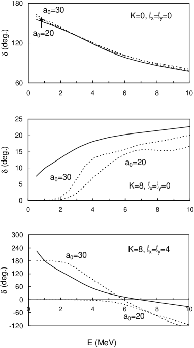
Figure 1: $\alpha$+n+n phase shifts ($J=0^{+}$) for channel radii $a_{0}=20$ fm $(N=20)$ and $a_{0}=30$ fm $(N=30)$, and for different partial waves. Solid lines are obtained with propagation up to $a=250$ fm of the $R$ matrix (curves corresponding to different $a_{0}$ are undistinguishable), and dashed lines without propagation.

Let us first illustrate the importance of the propagation technique. In Fig. 1, we plot some elements of the $J=0^{+}$ collision matrix under different conditions. In each case, we compare the phase shifts for two channel radii: $a_{0}=20$ fm and $a_{0}=30$ fm. The calculation is performed with and without propagation. For $K=0$, reasonable values can be obtained without propagation. However, for larger $K$ values ($K=8$ is displayed with $\ell_{x}=\ell_{y}=0$ and $\ell_{x}=\ell_{y}=4$), the channel radius should be quite large to reach convergence. To keep the same accuracy, the number of basis functions should be increased. However, one basis function per fm is a good estimate, and this leads to unrealistically large basis sizes. This convergence problem is due to the long range of the potential. The propagation technique (performed here up to $a=250$ fm) allows us to get a very high stability (better than $0.1^{\circ}$ at all energies) even for rather small channel radii. Consequently calculations with high $K$ values are still feasible.

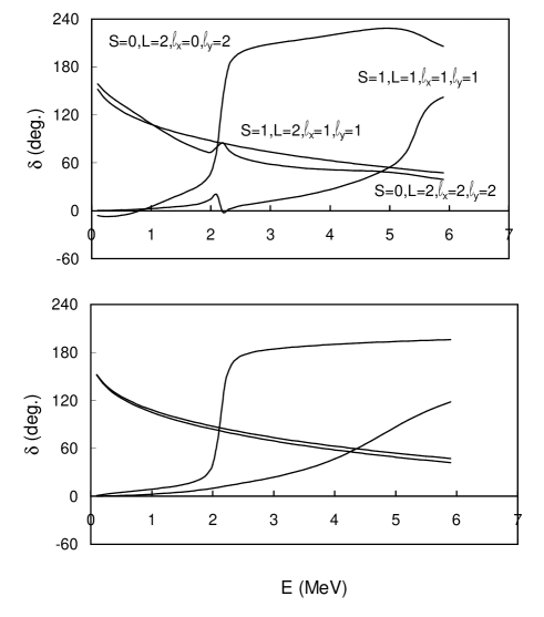
Figure 2: Diagonal phase shifts (upper panel) and eigenphases (lower panel) for the $\alpha$+n+n system ($J=2^{+},K_{max}=2$).

To illustrate the diagonalization of the collision matrix, we compare in Fig. 2 the diagonal phase shifts with the corresponding eigenphases. We have selected a particular case, with $J=2^{+}$, and $K_{max}=2$. With these conditions the collision matrix is $4\times 4$, and presents a narrow resonance near 2 MeV. In the upper part of Fig. 2, we plot the diagonal phase shifts. One of them presents a $180^{\circ}$ jump, characteristical of narrow resonances. This resonant behaviour is also observable in two other partial waves. After diagonalization of the collision matrix (Fig. 2, lower part) the resonant behaviour shows up in one eigenphase only. The three other eigenphases smoothly depend on energy.

The convergence with respect to $K_{max}$ is illustrated in Fig. 3 with the $J=0^{+}$ eigenphases. It turns out that, at low energies, high hypermomenta are necessary to achieve a precise convergence. However, above 4 MeV, $K_{max}=20$ is sufficient to obtain an accuracy of $2^{\circ}$.

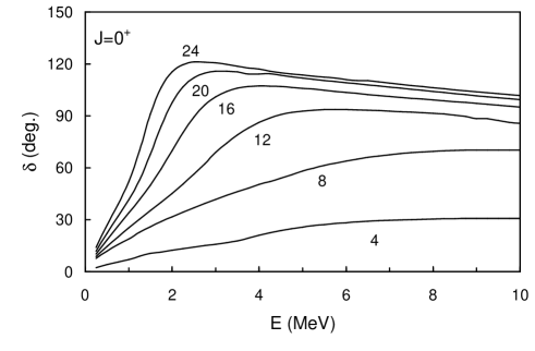
Figure 3: Energy dependence of $\alpha$+n+n eigenphases ($J=0^{+}$) for different $K_{max}$ values.

Figure 4 gives the eigenphases for $J=0^{+},1^{-},2^{+}$ in ⁶He and ⁶Be ($K_{max}$ is taken as 24, 19 and 16, respectively). As expected, the 2⁺ phase shift of ⁶He presents a narrow resonance. The theoretical energy (about 0.2 MeV) is however underestimated as the experimental value TCG02 is $E=0.82$ MeV. In order to provide meaningful properties for this state, we have readjusted the scaling factor to $\lambda=1.020$, which provides the correct energy. The 0⁺ and 1^- phase shifts show broad structures near 1.5 MeV. Similar phase shifts have been obtained by Danilin et al. DTV98 ; DRV04 and by Thompson et al. TDE00 with other potentials.

In ⁶Be, the ground state is found at $E=1.26$ MeV with a width $\Gamma=65$ keV. These values are in reasonable agreement with experiment TCG02 ($E=1.37$ MeV, $\Gamma=92\pm 6$ keV), the width being underestimated by the model due to the lower energy. Experimentally, a 2⁺ state is known near $E=3.0$ MeV with a width of $\Gamma=1.16\pm 0.06$ MeV. These properties are consistent with the theoretical 2⁺ eigenphase, which presents a broad structure near $E\approx 4$ MeV. The largest Coulomb eigenphases ($J=0^{+}$) are shown as dotted lines in Fig. 4. As expected, the Coulomb interaction plays a dominant role at low energies, but it cannot be completely neglected even near 10 MeV. Coulomb eigenphases for other spin values are very similar and therefore are not presented. Energies and widths are given in Table 2.

In Table 2, we also present the E2 transition probability in ⁶He. For the narrow $2^{+}$ resonance, we use the bound-state approximation. Without effective charge, the $B(E2)$ value for the $0^{+}\rightarrow 2^{+}$ transition is underestimated with respect to the experimental value AAA99 . However, the E2 matrix element is very sensitive to the effective charge. A small correction ($\delta e=0.05e$) provides a $B(E2)$ within the experimental error bars.

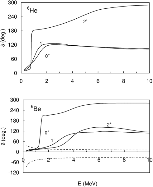
Figure 4: Eigenphases of ⁶He and ⁶Be for different $J$ values (solid lines). For ⁶Be, dotted lines represent the largest Coulomb eigenphases for $J=0^{+}$.

Table 2: ⁶He and ⁶Be properties. Unless specified, experimental data are taken from Ref. TCG02 .

	6He		6Be
	present	exp.	present	exp.
$E(0^{+})$ (MeV)	-0.97	-0.97	1.26	1.37
$\Gamma(0^{+})$ (keV)			65	$92\pm 6$
$E(2^{+})$ (MeV)	0.8	0.82	$\approx 4.0$	3.04
$\Gamma(2^{+})$ (MeV)	$0.04$	$0.113\pm 0.020$	$\approx 1.0$	$1.16\pm 0.06$
$\sqrt{<r^{2}>}$ (fm)	2.44	$2.33\pm 0.04^{a)}$
		$2.57\pm 0.10^{b)}$
		$2.45\pm 0.10^{c)}$
B(E2,$0^{+}\rightarrow 2^{+}$) ($e^{2}.$fm4)	1.23 ($\delta e=0$)	$3.2\pm 0.6^{d)}$
	2.69 ($\delta e=0.05e$)

^a) Ref. THH85 , ^b) Ref. Ch89 ^c) Ref. ADL04 , ^d) Ref. AAA99

III.3 Application to ¹⁴Be

As shown in previous works Ba97 ; ABD95 ; TZ96 , a ¹²Be+n+n three-body model can provide a realistic description of ¹⁴Be. The spectroscopy of the ¹⁴Be ground state has already been investigated in non-microscopic Ba97 ; ABD95 ; TZ96 ; TTT04 and microscopic De95 models. Here we extend three-body descriptions to ¹⁴Be excited and continuum states.

The ¹³Be ground state is expected to be a virtual $s$ wave, with a large and negative scattering length ($a_{s}<-10$ fm) TYH01 . In addition, the existence of a $5/2^{+}$ $d$-state near 2 MeV is well established. These properties can be reproduced by a ¹²Be-n potential

$$V(r)=-\frac{V_{0}+V_{s}\,\mbox{\boldmath$\ell\cdot s$}}{1+\exp((r-r_{0})/a)},$$ (50)

where $\ell$ is the relative angular momentum and $s$ the neutron spin. In Eq. (50), $r_{0}=2.908$ fm, $a=0.67$ fm, $V_{0}=43$ MeV, $V_{s}=6$ MeV. The range and diffuseness of the Woods-Saxon potential are taken from Ref. TZ96 . The amplitudes $V_{0}$ and $V_{s}$ provide $E(5/2^{+})=2.1$ MeV, and $a_{s}=-47$ fm, which are consistent with the data. For the n-n potential, we use the Minnesota interaction, as for the ⁶He study.

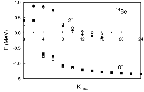
Figure 5: Energy of the ¹⁴Be $0^{+}$ (squares) and $2^{+}$ (circles) states as a function of $K_{max}$. Full symbols correspond to a renormalized ¹²Be-n potential, and open symbols to a phenomenological three-body term (see text).

With these potentials, the ¹⁴Be ground state is found at $E=-0.16$ MeV, which represents an underbinding with respect to experiment ($-1.34\pm 0.11$ MeV AW93 ). This calculation has been performed with $K_{max}=24$, which ensures the convergence. The underbinding problem is common to all three-body approaches, and can be solved in two ways. $(i)$ A renormalization factor $\lambda=1.08$ provides a ground-state energy at $-1.30$ MeV, i.e. within the experimental uncertainties. This procedure leads to a slightly bound ¹³Be ground state, which might influence the ¹⁴Be properties. $(ii)$ A three-body phenomenological term $V^{(123)}$, taken as in Ref. TDE00 , i.e.,

$$V^{(123)}_{K\gamma,K^{\prime}\gamma^{\prime}}(\rho)=-\delta_{KK^{\prime}}\delta_{\gamma\gamma^{\prime}}\,V_{3}/[1+(\rho/\rho_{3})^{2}],$$ (51)

reproduces the experimental energy with an amplitude $V_{3}=4.7$ MeV (according to Ref. TDE00 , we take $\rho_{3}=5$ fm). This potential is diagonal in $(K,\gamma)$, and is simply added to the two-body term [see Eqs. (10),(11)]. In ⁶He, it was shown that both readjustments of the interaction provide similar results DDB03 . However the renormalization factor is larger for ¹⁴Be, and both methods will be considered in the following.

The convergence with respect to $K_{max}$ is illustrated in Fig. 5. For $J=0^{+}$, the calculations have been done with $K_{max}$ up to 24. The energies obtained with renormalization or with the three-body potential are very similar. This confirms the conclusion drawn for the ⁶He nucleus DDB03 .

Table 3: Properties of the ¹⁴Be $0^{+}$ and $2^{+}$ states. $\lambda$ is the renormalization factor of the ¹²Be-n potential and $V_{3}$ is this amplitude of the three-body potential.

		$\lambda=1.08,V_{3}=0$	$\lambda=1,V_{3}=4.7$
$0^{+}$	$E$ (MeV)	$-1.34$	$-1.34$
	$\sqrt{<r^{2}>}$ (fm)	3.10	3.14
	$P_{S=1}$	0.046	0.033
$2^{+}$	$E$ (MeV)	$-0.15$	$-0.03$
	$\sqrt{<r^{2}>}$ (fm)	2.99	3.04
	$P_{S=1}$	0.192	0.165
$0^{+}\rightarrow 2^{+}$	B(E2) ($e^{2}$.fm4)	0.48 ($\delta e=0$)	0.64 ($\delta e=0$)
		3.18 ($\delta e=0.05e$)	4.05 ($\delta e=0.05e$)

Spectroscopic properties of ¹⁴Be are given in Tables 3 and 4. The r.m.s. radii have been determined with 2.57 fm as ¹²Be radius. For the ground state, we have $\sqrt{<r^{2}>}=3.10$ fm or 3.14 fm, in nice agreement with experiment ($3.16\pm 0.38$ fm, see Ref. TKY88 ). In all cases, the $S=1$ component (denoted as $P_{S=1}$) is small ($<5\%$). The decomposition in shell-model orbitals (see Table 4) shows that the $0^{+}$ state is essentially ($\approx 70\%$) $(2s_{1/2})^{2}$, with small $(2d_{3/2})^{2}$ and $(2d_{5/2})^{2}$ admixtures.

Table 4: Components (in %) in ¹⁴Be wave functions.

	$0^{+}(\lambda=1.08,V_{3}=0)$	$0^{+}(\lambda=1,V_{3}=4.7)$
$(p_{3/2})^{2}$	2.0	2.2
$(p_{1/2})^{2}$	1.0	1.1
$(s_{1/2})^{2}$	70.4	73.1
$(d_{5/2})^{2}$	14.6	13.0
$(d_{3/2})^{2}$	11.2	9.8
	$2^{+}(\lambda=1.08,V_{3}=0)$	$2^{+}(\lambda=1,V_{3}=4.7)$
$p_{3/2}p_{3/2}$	7.7	8.2
$p_{3/2}f_{7/2}$	9.6	9.4
$p_{1/2}p_{3/2}$	18.0	18.6
$p_{1/2}f_{5/2}$	5.8	5.7
$s_{1/2}d_{5/2}$	23.2	23.5
$s_{1/2}d_{3/2}$	19.2	18.5
$d_{5/2}d_{5/2}$	5.6	5.3
$d_{3/2}d_{5/2}$	4.0	3.6
$d_{3/2}d_{3/2}$	3.0	2.9

Regarding $J=2^{+}$, we have considered values up to $K_{max}=16$, where the number of partial waves is 172. Going beyond $K_{max}=16$ would require too large computer memories. Fig. 5 shows the energy convergence with respect to $K_{max}$. For both potentials, the energy is below threshold, and the r.m.s. radius is close to 3 fm. A partial-wave analysis provides 19% of $S=1$ admixture, a value much larger than in the ground state. Table 4 suggests that the structure of the 2⁺ state is spread over many components. The $(s_{1/2}d_{5/2})$ component is dominant ($\approx 23\%$) but other $(sd)$ and $(pf)$ orbitals also play a role.

E2 transition probabilities are also given in Table 3. Without effective charge, we have B(E2,$0^{+}\,\rightarrow\,2^{+}$) = 0.48 and 0.64 $e^{2}$fm⁴, which is lower than for the corresponding transition in ⁶He. However, the amplitudes of the proton and neutron E2 operators being even more different in ¹⁴Be than in ⁶He, the B(E2) values strongly depend on the effective charge. For $\delta e=0.05e$, we find B(E2) = 3.18 or 4.05 $e^{2}$fm⁴ according to the potential. Such transition probabilities should be measurable through Coulomb excitation experiments.

In Figs. 6-7, we present the 0⁺ and 2⁺ radial wave functions and probabilities $P(x,y)$ defined as

$$P^{J\pi}(x,y)=\int d\Omega_{x}\,d\Omega_{y}x^{2}y^{2}\mid\Psi^{JM\pi}(\mbox{\boldmath$x$},\mbox{\boldmath$y$})\mid^{2}.$$ (52)

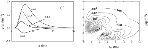
Figure 6: Left panel: radial functions $\chi(\rho)$ for the $0^{+}$ state. The curves are labeled by $\ell_{x},\ell_{y},n$. Right panel: probability $P(r_{nn},r_{Be-nn})$, deduced from Eq. (52) with $r_{nn}=\sqrt{2}x$ and $r_{Be-nn}=\sqrt{6/7}y$. Contour levels are plotted by steps of 0.005.

The dominant $S=0$ components are plotted. The $0^{+}$ probability shows two well distinct maxima, which resemble the maxima found in ⁶He, corresponding to ”dineutron” and ”cigar” configurations. Partial waves $\chi^{J\pi}_{\gamma K}(\rho)$ have maxima for $\rho>5$ fm. This corresponds to distances larger than in ⁶He DDB03 where the maxima of the main components are located near 4 fm. As expected, the 2⁺ probability is similar to the $0^{+}$ probability, with two maxima.

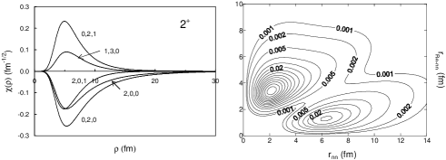
Figure 7: See Fig. 6 for the $2^{+}$ state.

Three-body eigenphases are displayed in Fig. 8. As for the ¹⁴Be spectroscopy the use of a three-body potential does not qualitatively change the phase shifts. The 1^- phase shift presents two jumps but they cannot be directly assigned to physical resonances. On the contrary, the 2⁺ phase shift shows a narrow resonance near 2 MeV. For the sake of completeness, ¹²O+p+p mirror phase shifts are also shown in Fig. 8. As expected, no narrow structure is found. A very broad 0⁺ resonance shows up near 8 MeV, and should correspond to the ¹⁴Ne ground state.

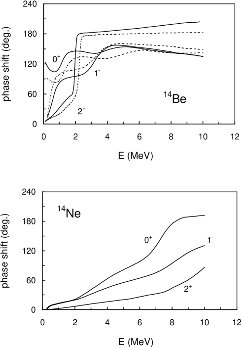
Figure 8: Three-body ¹²Be-n-n and ¹²O-p-p eigenphases. Solid lines correspond to a renormalized core-nucleon potential, and dotted lines to a phenomenological three-body term.

IV Conclusion

In this work, we have extended the three-body formalism of Ref. DDB03 to unbound states. As for two-body systems, the Lagrange-mesh technique, associated with the $R$-matrix method, provides an efficient and accurate way to derive collision matrices and wave functions. Compared with two-body systems, three-body $R$-matrix approaches are more tedious, owing to the coupling potentials which extend to very large distances. This behaviour is inherent to the use of hyperspherical coordinates which provide three-body potentials behaving as $1/\rho^{3}$, even for short-range two-body interactions. This problem can be efficiently solved by using propagation techniques. Here, we propagate the wave function and the $R$ matrix by using the Numerov algorithm. This formalism has been extended to charged systems.

The ⁶He system has essentially been used as a test of the method, as most of its properties are available in the literature. The $B(E2,0^{+}\rightarrow 2^{+})$ experimental value can be reproduced with a small effective charge $\delta e=0.05e$. We have determined $\alpha$+p+p phase shifts, and found a good agreement with experiment for the ⁶Be ground-state properties.

Application to three-body ¹²Be+n+n states is new, and has been developed in two directions. The bound-state description of ¹⁴Be provides evidence for a 2⁺ bound state, as expected from the shell model. The study of the ¹²Be+n+n system has been complemented by three-body phase shifts, which suggest the existence of a second narrow $2^{+}$ resonance at $E_{x}\approx 3.4$ MeV.

A limitation of the method is the slow convergence of the phase shifts with respect to the maximum hypermomentum $K_{max}$. To achieve a full convergence, values up to $K_{max}$ = 20 or more are necessary. This problem is even stronger for high spins, where the number of partial waves increases rapidly. A possible solution to this problem would be to apply the Feshbach reduction method Fe62 to scattering states. Another possible development would be to use a projection technique to remove Pauli forbidden states KK77 . In that case, asymptotic potentials (19) are non local, which makes the calculation still heavier.

The present model offers an efficient way to investigate bound and unbound states. In exotic nuclei, most low-lying states are unbound, and a rigorous analysis requires scattering conditions. The inclusion of the Coulomb interaction still extends the application field, and is interesting even for non-exotic nuclei. In this context, an accurate analysis of unbound $\alpha+\alpha+\alpha$ states seems desirable in view of its strong interest in the triple-$\alpha$ reaction rate fynbo05 .

References

- (1) B. Jonson, Phys. Rep. 389 (2004) 1.
- (2) M.V. Zhukov, B.V. Danilin, D.V. Fedorov, J.M. Bang, I.J. Thompson, J.S. Vaagen, Phys. Rep. 231 (1993) 151.
- (3) I. Tanihata, H. Hamagaki, O. Hashimoto, Y. Shida, N. Yoshikawa, K. Sugimoto, O. Yamakawa, T. Kobayashi, N. Takahashi, Phys. Rev. Lett. 55 (1985) 2676.
- (4) P.M. Morse, H. Feshbach, Methods in Theoretical Physics, vol. II, McGraw-Hill, New York, (1953).
- (5) C.D. Lin, Phys. Rep. 257 (1995) 1.
- (6) P. Descouvemont, C. Daniel, D. Baye, Phys. Rev. C 67 (2003) 044309.
- (7) D. Baye, M. Hesse, M. Vincke, Phys. Rev. E 65 (2002) 026701.
- (8) T. Aumann et al., Phys. Rev. C 59 (1999) 1252.
- (9) Y.K. Ho, Phys. Rep. 99 (1983) 1.
- (10) V.I. Kukulin, V.M. Krasnopol’sky, J. Phys. A 10 (1977) 33.
- (11) A.M. Lane, R.G. Thomas, Rev. Mod. Phys. 30 (1958) 257.
- (12) I.J. Thompson, B.V. Danilin, V.D. Efros, J.S. Vaagen, J.M. Bang, M.V. Zhukov, Phys. Rev. C 61 (2000) 024318.
- (13) V.M. Burke, C.J. Noble, Comput. Phys. Commun. 85 (1995) 471.
- (14) D. Baye, M. Hesse, J.-M. Sparenberg, M. Vincke, J. Phys. B 31 (1998) 3439.
- (15) M. Hesse, J.-M. Sparenberg, F. Van Raemdonck, D Baye, Nucl. Phys. A 640 (1998) 37.
- (16) J. Raynal, J. Revai, Nuovo. Cim. A 39 (1970) 612.
- (17) V. Vasilevsky, A.V. Nesterov, F. Arickx, J. Broeckhove, Phys. Rev. C 63 (2001) 034606.
- (18) M. Abramowitz, I.A. Stegun, Handbook of Mathematical Functions, Dover, London (1972).
- (19) H. Kanada, T. Kaneko, S. Nagata, M. Nomoto, Prog. Theor. Phys. 61 (1979) 1327.
- (20) D. Baye, Phys. Rev. Lett. 58 (1987) 2738.
- (21) I.J. Thompson, A.R. Barnett, J. Comput. Phys. 64 (1986) 490.
- (22) J. Raynal, in ”Computing as a Language of Physics”, Trieste 1971, IAEA, Vienna, (1972) p. 281.
- (23) M. Gailitis, J. Phys. B9 (1976) 843.
- (24) D. Baye, P. Descouvemont, Nucl. Phys. A 407 (1983) 77.
- (25) P. Descouvemont, M. Vincke, Phys. Rev. A 42 (1990) 3835.
- (26) M. Hesse, J. Roland, D. Baye, Nucl. Phys. A 709 (2002) 184.
- (27) V.I. Kukulin, V.N. Pomerantsev, Ann. Phys. 111 (1978) 330.
- (28) D.R. Thompson, M. LeMere, Y.C. Tang, Nucl. Phys. A 286 (1977) 53.
- (29) D.R. Tilley, C.M. Cheves, J.L. Godwin, G.M. Hale, H.M. Hofmann, J.H. Kelley, C.G. Sheua, H.R. Weller, Nucl. Phys. A 708 (2002) 3.
- (30) B.V. Danilin, I.J. Thompson, J.S. Vaagen, M.V. Zhukov, Nucl. Phys. A 632 (1998) 383.
- (31) B.V. Danilin, T. Rogde, J.S. Vaagen, I.J. Thompson, M.V. Zhukov, Phys. Rev. C 69 (2004) 024609.
- (32) L.V. Chulkov et al., Europhys. Lett. 8 (1989) 245.
- (33) G.D. Alkhazov, A.V. Dobrovolsky, A.A. Lobodenko, Nucl. Phys. A 734 (2004) 361.
- (34) D. Baye, Nucl. Phys. A 627 (1997) 305.
- (35) A. Adahchour, D. Baye, P. Descouvemont, Phys. Lett. B 356 (1995) 445.
- (36) I.J. Thompson, M.V. Zhukov, Phys. Rev. C 53 (1996) 708.
- (37) T. Tarutina, I.J. Thompson, J.A. Tostevin, Nucl. Phys. A 733 (2004) 53.
- (38) P. Descouvemont, Phys. Rev. C 52 (1995) 704.
- (39) M. Thoennessen, S. Yokoyama, P.G. Hansen, Phys. Rev. C 63 (2001) 014308.
- (40) G. Audi, A.H. Wapstra, Nucl. Phys. A 565 (1993) 1.
- (41) I. Tanihata, T. Kobayashi, O. Yamakawa, S. Shimoura, K. Ekuni, K. Sugimoto, N. Takahashi, T. Shimoda, H. Sato, Phys. Lett. B 206 (1988) 592.
- (42) H. Feshbach, Ann. Phys. 19 (1962) 287.
- (43) H. Fynbo et al., Nature 433 (2005) 136.