Critical Point Symmetries (CPS) appear in regions of the nuclear chart where a rapid change from one symmetry to another is observed. The first CPSs, introduced by F. Iachello, were E(5), which corresponds to the transition from vibrational [U(5)] to $\gamma$-unstable [O(6)] behaviour, and X(5), which represents the change from vibrational [U(5)] to prolate axially deformed [SU(3)] shapes. These CPSs have been obtained as special solutions of the Bohr collective Hamiltonian. More recent special solutions of the same Hamiltonian, to be described here, include Z(5) and Z(4), which correspond to maximally triaxial shapes (the latter with “frozen” $\gamma=30^{\rm o}$), as well as X(3), which corresponds to prolate shapes with “frozen” $\gamma=0^{\rm o}$. CPSs have the advantage of providing predictions which are parameter free (up to overall scale factors) and compare well to experiment. However, their mathematical structure [with the exception of E(5)] needs to be clarified.

1 Introduction

Critical point symmetries [1, 2], describing nuclei at points of shape phase transitions between different limiting symmetries, have recently attracted considerable attention, since they lead to parameter independent (up to overall scale factors) predictions which are found to be in good agreement with experiment [3, 4, 5, 6, 7]. The E(5) critical point symmetry [1] is supposed to correspond to the transition from vibrational [U(5)] to $\gamma$-unstable [O(6)] nuclei, while the X(5) critical point symmetry [2] is assumed to describe the transition from vibrational [U(5)] to prolate axially symmetric [SU(3)] nuclei. Both symmetries are obtained as special solutions of the Bohr Hamiltonian [8]. In the E(5) case [1] the potential is supposed to depend only on the collective variable $\beta$ and not on $\gamma$. Then exact separation of variables is achieved and the equation containing $\beta$ can be solved exactly [1, 9] for an infinite square well potential in $\beta$, the eigenfunctions being Bessel functions of the first kind, while the equation containing the angles has been solved a long time ago by Bès [10]. In the X(5) case [2] the potential is supposed to be of the form $u(\beta)+u(\gamma)$. Then approximate separation of variables is achieved in the special case of $\gamma\simeq 0$, the $\beta$-equation with an infinite square well potential leading to Bessel eigenfunctions, while the $\gamma$-equation with a harmonic oscillator potential having a minimum at $\gamma=0$ leads to a two-dimensional harmonic oscillator with Laguerre eigenfunctions [2]. In both cases the full five variables of the Bohr Hamiltonian [8] (the collective variables $\beta$ and $\gamma$, as well as the three Euler angles) are involved. The algebraic structure of E(5) is clear, since the Hamiltonian is the second order Casimir operator of E(5), which corresponds to the square of the momentum operator in five dimensions (see [11, 12] and references therein), while an SO(5) subalgebra (generated by the angular momentum operators in five dimensions) exists. The algebraic structure of X(5) (if any, since X(5) is an approximate and not an exact solution) has not been identified yet.

It is of interest to identify additional special cases leading to analytical solutions of the Bohr Hamiltonian, and to examine their relation to critical behaviour of nuclei, clarifying in parallel their algebraic structure.

It has been known for a long time that the Bohr equation gets simplified in the special case of $\gamma=30^{\rm o}$ [13, 14], since two of the principal moments of inertia become equal in this case, guaranteeing the existence of a good quantum number (the projection $\alpha$ of angular momentum on the body-fixed $\hat{x}^{\prime}$ axis), although the nucleus possesses a triaxial shape. In other words, the Hamiltonian possesses a symmetry, while the shape of the nucleus does not. By allowing the potential to be of the form $u(\beta)+u(\gamma)$, and by permitting $\gamma$ to vary only around $\gamma\simeq 30^{\rm o}$, approximate separation of variables is achieved [15], similar in spirit to the X(5) solution. The $\beta$-equation with an infinite square well potential leads then to Bessel eigenfunctions, while the $\gamma$-equation with a harmonic oscillator potential having a minimum at $\gamma=30^{\rm o}$ takes the form of a simple harmonic oscillator equation. The full five variables of the Bohr Hamiltonian are involved in this case, while the algebraic structure (if any, since the solution is approximate) is yet unknown. This solution, which has been called Z(5) [15], is presented in Section 2.

Separation of variables becomes exact by “freezing” the $\gamma$ variable to the special value of $\gamma=30^{\rm o}$, in the spirit of the Davydov and Chaban [16] approach. Then the $\beta$-equation with an infinite square well potential leads to Bessel eigenfunctions [12], while the equation involving the Euler angles and the parameter $\gamma$ (which is not a variable any more) leads to the solution obtained by Meyer-ter-Vehn [14]. The projection $\alpha$ of angular momentum on the body-fixed $\hat{x}^{\prime}$ axis is a good quantum number also in this case. Only four variables ($\beta$ and the three Euler angles) are involved, while the full algebraic structure is yet unknown. It has been remarked [12], however, that the ground state band of this model coincides with the ground state band of E(4), the Euclidean algebra in four dimensions. This solution, which has been labelled as Z(4) [12], is presented in Section 3.

The question arises then of what happens in the case one “freezes” the $\gamma$ variable to the value $\gamma=0$, which corresponds to axially symmetric prolate shapes, for which the projection $K$ of angular momentum on the body-fixed $\hat{z}$-axis is a good quantum number. It turns out [17] that only three degrees of freedom are relevant in this case, since the nucleus is axially symmetric, so that two angles suffice for describing its direction in space, while the variable $\beta$ describes its shape. Separation of variables becomes exact [17], the $\beta$ equation with an infinite square well potential leading to Bessel eigenfunctions, while the equation involving the angles leads to the simple spherical harmonics. The algebraic structure of this model is yet unknown. This solution, which has been called X(3) [17], is presented in Section 4.

Finally, in Section 5 the present results are briefly discussed and plans for further work are exposed.

2 The Z(5) model

The original Bohr Hamiltonian [8] is

$$H=-{\hbar^{2}\over 2B}\left[{1\over\beta^{4}}{\partial\over\partial\beta}\beta^{4}{\partial\over\partial\beta}+{1\over\beta^{2}\sin 3\gamma}{\partial\over\partial\gamma}\sin 3\gamma{\partial\over\partial\gamma}\right.$$

$$\left.-{1\over 4\beta^{2}}\sum_{k=1,2,3}{Q_{k}^{2}\over\sin^{2}\left(\gamma-{2\over 3}\pi k\right)}\right]+V(\beta,\gamma),$$ (1)

where $\beta$ and $\gamma$ are the usual collective coordinates, while $Q_{k}$ ($k=1$, 2, 3) are the components of angular momentum in the intrinsic coordinate system and $B$ is the mass parameter.

In the case in which the potential has a minimum around $\gamma=\pi/6$ one can write the last term of Eq. (1) in the form $4(Q_{1}^{2}+Q_{2}^{2}+Q_{3}^{2})-3Q_{1}^{2}$. Using this result in the Schrödinger equation corresponding to the Hamiltonian of Eq. (1), introducing [1] reduced energies $\epsilon=2BE/\hbar^{2}$ and reduced potentials $u=2BV/\hbar^{2}$, and assuming [2] that the reduced potential can be separated into two terms, one depending on $\beta$ and the other depending on $\gamma$, i.e. $u(\beta,\gamma)=u(\beta)+u(\gamma)$, the Schrödinger equation can be separated into two equations

$$\left[-{1\over\beta^{4}}{\partial\over\partial\beta}\beta^{4}{\partial\over\partial\beta}+{1\over 4\beta^{2}}(4L(L+1)-3\alpha^{2})+u(\beta)\right]\xi_{L,\alpha}(\beta)=\epsilon_{\beta}\xi_{L,\alpha}(\beta),$$ (2)

$$\left[-{1\over\langle\beta^{2}\rangle\sin 3\gamma}{\partial\over\partial\gamma}\sin 3\gamma{\partial\over\partial\gamma}+u(\gamma)\right]\eta(\gamma)=\epsilon_{\gamma}\eta(\gamma),$$ (3)

where $L$ is the angular momentum quantum number, $\alpha$ is the projection of the angular momentum on the body-fixed $\hat{x}^{\prime}$-axis ($\alpha$ has to be an even integer [14]), $\langle\beta^{2}\rangle$ is the average of $\beta^{2}$ over $\xi(\beta)$, and $\epsilon=\epsilon_{\beta}+\epsilon_{\gamma}$.

The total wave function should have the form $\Psi(\beta,\gamma,\theta_{i})=\xi_{L,\alpha}(\beta)\eta(\gamma){\cal D}^{L}_{M,\alpha}(\theta_{i})$, where $\theta_{i}$ ($i=1$, 2, 3) are the Euler angles, ${\cal D}(\theta_{i})$ denote Wigner functions of them, $L$ is the angular momentum quantum number, while $M$ and $\alpha$ are the eigenvalues of the projections of angular momentum on the laboratory fixed $\hat{z}$-axis and the body-fixed $\hat{x}^{\prime}$-axis respectively.

Instead of the projection $\alpha$ of the angular momentum on the $\hat{x}^{\prime}$-axis, it is customary to introduce the wobbling quantum number [14, 18] $n_{w}=L-\alpha$. Inserting $\alpha=L-n_{w}$ in Eq. (2) one obtains

$$\left[-{1\over\beta^{4}}{\partial\over\partial\beta}\beta^{4}{\partial\over\partial\beta}+{1\over 4\beta^{2}}(L(L+4)+3n_{w}(2L-n_{w}))+u(\beta)\right]\xi_{L,n_{w}}(\beta)$$

$$=\epsilon_{\beta}\xi_{L,n_{w}}(\beta),$$ (4)

where the wobbling quantum number $n_{w}$ labels a series of bands with $L=n_{w},n_{w}+2,n_{w}+4,\dots$ (with $n_{w}>0$) next to the ground state band (with $n_{w}=0$) [14].

In the case in which $u(\beta)$ is an infinite well potential

$$u(\beta)=\left\{\begin{array}[]{ll}0&\mbox{if $\beta\leq\beta_{W}$}\\ \infty&\mbox{for $\beta>\beta_{W}$}\end{array}\right.,$$ (5)

one can use the transformation [2] $\tilde{\xi}(\beta)=\beta^{3/2}\xi(\beta)$, as well as the definitions [2] $\epsilon_{\beta}=k_{\beta}^{2}$, $z=\beta k_{\beta}$, in order to bring Eq. (4) into the form of a Bessel equation

$${d^{2}\tilde{\xi}\over dz^{2}}+{1\over z}{d\tilde{\xi}\over dz}+\left[1-{\nu^{2}\over z^{2}}\right]\tilde{\xi}=0,$$ (6)

with

$$\nu={\sqrt{4L(L+1)-3\alpha^{2}+9}\over 2}={\sqrt{L(L+4)+3n_{w}(2L-n_{w})+9}\over 2}.$$ (7)

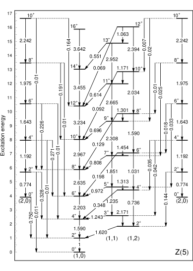
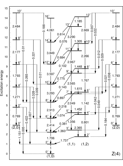
Figure 1: (a) Intraband and interband B(E2) transition rates in the Z(5) model [15], normalized to the B(E2;$2_{1,0}\to 0_{1,0}$) rate. Bands are labelled by $(s,n_{w})$, their levels being normalized to $2_{1,0}$. The (2,0) band is shown both at the left and at the right end of the figure for drawing purposes. (b) Same for the Z(4) model [12].

Then the boundary condition $\tilde{\xi}(\beta_{W})=0$ determines the spectrum

$$\epsilon_{\beta;s,\nu}=\epsilon_{\beta;s,n_{w},L}=(k_{s,\nu})^{2},\qquad k_{s,\nu}=x_{s,\nu}/\beta_{W},$$ (8)

and the eigenfunctions

$$\xi_{s,\nu}(\beta)=\xi_{s,n_{w},L}(\beta)=\xi_{s,\alpha,L}(\beta)=c_{s,\nu}\beta^{-3/2}J_{\nu}(k_{s,\nu}\beta),$$ (9)

where $x_{s,\nu}$ is the $s$th zero of the Bessel function $J_{\nu}(z)$, while the normalization constants $c_{s,\nu}$ are determined from the normalization condition $\int_{0}^{\infty}\beta^{4}\xi^{2}_{s,\nu}(\beta)d\beta=1$. The notation for the roots has been kept the same as in Ref. [2], while for the energies the notation $E_{s,n_{w},L}$ will be used. The ground state band corresponds to $s=1$, $n_{w}=0$. We shall refer to the model corresponding to this solution as Z(5) (which is not meant as a group label), in analogy to the E(5) [1] and X(5) [2] models.

The $\gamma$-part of the spectrum is obtained from Eq. (3), which, in the case of a harmonic oscillator potential having a minimum at $\gamma=\pi/6$, takes the form of a simple harmonic oscillator equation [15]. Similar potentials and solutions in the $\gamma$-variable have been considered in [8]. The total energy in the case of the Z(5) model is then

$$E(s,n_{w},L,n_{\tilde{\gamma}})=E_{0}+A(x_{s,\nu})^{2}+Bn_{\tilde{\gamma}},$$ (10)

where $n_{\tilde{\gamma}}$ is the quantum number of the oscillator occuring in the $\gamma$-equation.

The calculation of B(E2) transition rates has been described in detail in Ref. [15]. The resulting level scheme is shown in Fig. 1(a). Experimental manifestations of Z(5) seem to appear in the ^192-196Pt region [15].

3 The Z(4) model

3.1 The Z(4) solution

In the model of Davydov and Chaban [16] it is assumed that the nucleus is rigid with respect to $\gamma$-vibrations. Then the Hamiltonian depends on four variables ($\beta,\theta_{i}$) and has the form [16]

$$H=-\frac{\hbar^{2}}{2B}\Biggl{[}\frac{1}{\beta^{3}}\frac{\partial}{\partial\beta}\beta^{3}\frac{\partial}{\partial\beta}-\frac{1}{4\beta^{2}}\sum_{k=1}^{3}\frac{Q_{k}^{2}}{\sin^{2}(\gamma-\frac{2\pi}{3}k)}\Biggr{]}+U(\beta).$$ (11)

In this Hamiltonian $\gamma$ is treated as a parameter and not as a variable. The kinetic energy term of Eq. (11) is different from the one appearing in the E(5) and X(5) models, because of the different number of degrees of freedom treated in each case (four in the former case, five in the latter).

Introducing [1] reduced energies $\epsilon=(2B/\hbar^{2})E$ and reduced potentials $u=(2B/\hbar^{2})U$, and considering a wave function of the form $\Psi(\beta,\theta_{i})=\phi(\beta)\psi(\theta_{i})$, where $\theta_{i}$ ( $i=1$, 2, 3) are the Euler angles, separation of variables leads to two equations

$$\Biggl{[}\frac{1}{\beta^{3}}\frac{\partial}{\partial\beta}\beta^{3}\frac{\partial}{\partial\beta}-\frac{\lambda}{\beta^{2}}+(\epsilon-u(\beta))\Biggr{]}\phi(\beta)=0,$$ (12)

$$\Biggl{[}\frac{1}{4}\sum_{k=1}^{3}\frac{Q_{k}^{2}}{\sin^{2}(\gamma-\frac{2\pi}{3}k)}-\lambda\Biggr{]}\psi(\theta_{i})=0.$$ (13)

In the case of $\gamma=\pi/6$, the last equation takes the form

$$\Biggl{[}\frac{1}{4}(Q_{1}^{2}+4Q_{2}^{2}+4Q_{3}^{2})-\lambda\Biggr{]}\psi(\theta_{i})=0.$$ (14)

This equation has been solved by Meyer-ter-Vehn [14], the eigenfunctions being

$$\psi(\theta_{i})=\psi^{L}_{\mu,\alpha}(\theta_{i})=\sqrt{\frac{2L+1}{16\pi^{2}(1+\delta_{\alpha,0})}}\,\Bigl{[}{\cal D}^{(L)}_{\mu,\alpha}(\theta_{i})+(-1)^{L}{\cal D}^{(L)}_{\mu,-\alpha}(\theta_{i})\Bigr{]}$$ (15)

with

$$\lambda=\lambda_{L,\alpha}=L(L+1)-\frac{3}{4}\,\alpha^{2},$$ (16)

where $\mu$ and $\alpha$ are the eigenvalues of the projections of angular momentum on the laboratory fixed $\hat{z}$-axis and the body-fixed $\hat{x}^{\prime}$-axis respectively. $\alpha$ has to be an even integer [14]. As in the previous section, the wobbling quantum number, $n_{w}$ [14, 18], is introduced at this point.

The “radial” Eq. (12) is exactly soluble in the case of an infinite square well potential [Eq. (5)]. Using the transformation $\phi(\beta)=\beta^{-1}f(\beta)$, Eq. (12) becomes a Bessel equation

$$\Biggl{[}\frac{\partial^{2}}{\partial\beta^{2}}+\frac{1}{\beta}\frac{\partial}{\partial\beta}+\Bigl{(}\epsilon-\frac{\nu^{2}}{\beta^{2}}\Bigr{)}\Biggr{]}f(\beta)=0,$$ (17)

with

$$\nu=\sqrt{\lambda+1}={\sqrt{L(L+4)+3n_{w}(2L-n_{w})+4}\over 2}.$$ (18)

Then the boundary condition $f(\beta_{W})=0$ determines the spectrum, which is given by Eq. (8), while the eigenfunctions are

$$\phi(\beta)=\phi_{s,\nu}(\beta)=\phi_{s,n_{w},L}(\beta)=\frac{1}{\sqrt{c}}\,\beta^{-1}J_{\nu}(k_{s,\nu}\beta),\quad c=\frac{\beta_{W}^{2}}{2}\,J^{2}_{\nu+1}(x_{s,\nu})$$ (19)

where the normalization constant $c$ is determined from the condition $\int_{0}^{\beta_{W}}\beta^{3}\phi^{2}(\beta)d\beta=1$. The notation for the roots has been kept the same as in Ref. [2], while for the energies the notation $E_{s,n_{w},L}$ will be used. The ground state band corresponds to $s=1$, $n_{w}=0$. This model will be called the Z(4) model.

The calculation of B(E2)s proceeds as described in Refs. [12, 15]. The resulting level scheme is shown in Fig. 1(b). Experimental manifestations of Z(4) seem to appear in the ^128-132Xe region [12]. One can easily see that the spectra of the ground state band and the $\beta_{1}$ band, as well as the related transitions, are very similar to the ones predicted by the E(5) model [1, 11], while for the $\gamma_{1}$ bands the odd levels are very similar, while the even levels exhibit opposite staggering [12]. A partial explanation of this behaviour is given in the next subsection.

3.2 Relation of the ground state band of Z(4) to E(4)

The ground state band of the Z(4) model is related to the second order Casimir operator of E(4), the Euclidean algebra in four dimensions. In order to see this, one can consider in general the Euclidean algebra in $n$ dimensions, E(n), which is the semidirect sum [19] of the algebra T_n of translations in $n$ dimensions, generated by the momenta $P_{j}=-i\partial/\partial x_{j}$, and the SO(n) algebra of rotations in $n$ dimensions, generated by the angular momenta

$$L_{jk}=-i\left(x_{j}{\partial\over\partial x_{k}}-x_{k}{\partial\over\partial x_{j}}\right),$$ (20)

symbolically written as E(n) = T_n $\oplus_{s}$ SO(n) [20]. The generators of E(n) satisfy the commutation relations

$$[P_{i},P_{j}]=0,\qquad[P_{i},L_{jk}]=i(\delta_{ik}P_{j}-\delta_{ij}P_{k}),$$ (21)

$$[L_{ij},L_{kl}]=i(\delta_{ik}L_{jl}+\delta_{jl}L_{ik}-\delta_{il}L_{jk}-\delta_{jk}L_{il}).$$ (22)

From these commutation relations one can see that the square of the total momentum, $P^{2}$, is a second order Casimir operator of the algebra, while the eigenfunctions of this operator satisfy the equation

$$\left(-{1\over r^{n-1}}{\partial\over\partial r}r^{n-1}{\partial\over\partial r}+{\omega(\omega+n-2)\over r^{2}}\right)F(r)=k^{2}F(r),$$ (23)

in the left hand side of which the eigenvalues of the Casimir operator of SO(n), $\omega(\omega+n-2)$ appear [21]. Putting $F(r)=r^{(2-n)/2}f(r)$ and $\nu=\omega+(n-2)/2$, Eq. (23) is brought into the form

$$\left({\partial^{2}\over\partial r^{2}}+{1\over r}{\partial\over\partial r}+k^{2}-{\nu^{2}\over r^{2}}\right)f(r)=0,$$ (24)

the eigenfunctions of which are the Bessel functions $f(r)=J_{\nu}(kr)$. The similarity between Eqs. (24) and (17) is clear.

The ground state band of Z(4) is characterized by $n_{w}=0$, which means that $\alpha=L$. Then Eq. (18) leads to $\nu=L/2+1$, while in the case of E(4) one has $\nu=\omega+1$. Then the two results coincide for $L=2\omega$, i.e. for even values of $L$. One can easily see that this coincidence occurs only in four dimensions.

It should be emphasized, however, that neither the similarity of spectra and B(E2) values of Z(4) to these of the E(5) model, nor the coincidence of the ground state band of Z(4) to the spectrum of the Casimir operator of the Euclidean algebra E(4) clarify the algebraic structure of the Z(4) model, the symmetry algebra of which has to be constructed explicitly, starting from the fact that $\gamma$ is fixed to $30^{\rm o}$, for which the Bohr Hamiltonian possesses “accidentally” a symmetry axis (the body-fixed $\hat{x}^{\prime}$-axis).

4 The X(3) model

In the collective model of Bohr [8] the classical expression of the kinetic energy corresponding to $\beta$ and $\gamma$ vibrations of the nuclear surface plus rotation of the nucleus has the form [8, 22]

$$T=\frac{1}{2}\sum_{k=1}^{3}{\cal J}_{k}\,\omega^{\prime 2}_{k}+\frac{B}{2}\,(\dot{\beta}^{2}+\beta^{2}\dot{\gamma}^{2}),$$ (25)

where $\beta$ and $\gamma$ are the usual collective variables, $B$ is the mass parameter,

$${\cal J}_{k}=4B\beta^{2}\sin^{2}\bigl{(}\gamma-2\pi k/3\bigr{)}$$

are the three principal irrotational moments of inertia, and $\omega^{\prime}_{k}$ ($k=1$, 2, 3) are the components of the angular velocity on the body-fixed $\hat{k}$-axes, which can be expressed in terms of the time derivatives of the Euler angles $\dot{\phi},\dot{\theta},\dot{\psi}$ [22, 23]

$$\omega^{\prime}_{1}=-\sin\theta\cos\psi\,\dot{\phi}+\sin\psi\,\dot{\theta},\,\omega^{\prime}_{2}=\sin\theta\sin\psi\,\dot{\phi}+\cos\psi\,\dot{\theta},\,\omega^{\prime}_{3}=\cos\theta\,\dot{\phi}+\dot{\psi}.$$ (26)

Assuming the nucleus to be $\gamma$-rigid (i.e. $\dot{\gamma}=0$), as in the Davydov and Chaban approach [16], and considering in particular the axially symmetric prolate case of $\gamma=0$, we see that the third irrotational moment of inertia ${\cal J}_{3}$ vanishes, while the other two become equal (${\cal J}_{1}={\cal J}_{2}=3B\beta^{2}$), the kinetic energy of Eq. (25) reaching the form [22, 24]

$$T=\frac{1}{2}3B\beta^{2}(\omega^{\prime 2}_{1}+\omega^{\prime 2}_{2})+\frac{B}{2}\,\dot{\beta}^{2}=\frac{B}{2}\Bigl{[}3\beta^{2}(\sin^{2}\theta\,\dot{\phi}^{2}+\dot{\theta}^{2})+\dot{\beta}^{2}\Bigr{]}.$$ (27)

It is clear that in this case the motion is characterized by three degrees of freedom. Introducing the generalized coordinates $q_{1}=\phi$, $q_{2}=\theta$, and $q_{3}=\beta$, the kinetic energy becomes a quadratic form of the time derivatives of the generalized coordinates [22, 25] $T=B\sum_{i,j=1}^{3}g_{ij}\;\dot{q}_{i}\dot{q}_{j}/2$, with the matrix $g_{ij}$ having a diagonal form

$$g_{ij}=\left(\begin{array}[]{ccc}3\beta^{2}\sin^{2}\theta&0&0\\ 0&3\beta^{2}&0\\ 0&0&1\end{array}\right).$$ (28)

(In the case of the full Bohr Hamiltonian [8] the square matrix $g_{ij}$ is 5-dimensional and non-diagonal [22, 25].)

Figure 2: Energy levels of the ground state ($s=1$), $\beta_{1}$ ($s=2$), and $\beta_{2}$ ($s=3$) bands of X(3) [17], normalized to the energy of the lowest excited state, $2_{1}^{+}$, together with intraband $B(E2)$ transition rates, normalized to the transition between the two lowest states, $B(E2;2_{1}^{+}\to 0_{1}^{+})$. Interband transitions are listed in Table 1.

Following the general procedure of quantization in curvilinear coordinates one obtains the Hamiltonian operator [22, 25]

$$H=-\frac{\hbar^{2}}{2B}\,\Delta+U(\beta)=-\frac{\hbar^{2}}{2B}\Biggl{[}\frac{1}{\beta^{2}}\frac{\partial}{\partial\beta}\beta^{2}\frac{\partial}{\partial\beta}+\frac{1}{3\beta^{2}}\Delta_{\Omega}\Biggr{]}+U(\beta),$$ (29)

where $\Delta_{\Omega}$ is the angular part of the Laplace operator

$$\Delta_{\Omega}=\frac{1}{\sin\theta}\frac{\partial}{\partial\theta}\sin\theta\frac{\partial}{\partial\theta}+\frac{1}{\sin^{2}\theta}\frac{\partial^{2}}{\partial\phi^{2}}.$$ (30)

The Schrödinger equation can be solved by the factorization

$$\Psi(\beta,\theta,\phi)=F(\beta)\,Y_{LM}(\theta,\phi),$$ (31)

where $Y_{LM}(\theta,\phi)$ are the spherical harmonics. Then the angular part leads to the equation

$$-\Delta_{\Omega}Y_{LM}(\theta,\phi)=L(L+1)Y_{LM}(\theta,\phi),$$ (32)

where $L$ is the angular momentum quantum number, while for the radial part $F(\beta)$ one obtains

$$\Biggl{[}\frac{1}{\beta^{2}}\frac{d}{d\beta}\beta^{2}\frac{d}{d\beta}-\frac{L(L+1)}{3\beta^{2}}+\frac{2B}{\hbar^{2}}\Bigl{(}E-U(\beta)\Bigr{)}\Biggr{]}F(\beta)=0.$$ (33)

As in the case of X(5) [2], the potential in $\beta$ is taken to be an infinite square well [Eq. (5]. In this case $F(\beta)$ is a solution of the equation

$$\Biggl{[}\frac{d^{2}}{d\beta^{2}}+\frac{2}{\beta}\frac{d}{d\beta}+\Biggl{(}k^{2}-\frac{L(L+1)}{3\beta^{2}}\Biggr{)}\Biggr{]}F(\beta)=0$$ (34)

in the interval $0\leq\beta\leq\beta_{W}$, where reduced energies $\varepsilon=k^{2}=2BE/\hbar^{2}$ [2] have been introduced, while it vanishes outside.

Table 1: Interband $B(E2;L_{i}\to L_{f})$ transition rates for the X(3) model [17], normalized to the one between the two lowest states, $B(E2;2_{1}^{+}\to 0_{1}^{+})$.

$L_{i}\to L_{f}$	X(3)	$L_{i}\to L_{f}$	X(3)	$L_{i}\to L_{f}$	X(3)
$0_{2}\to 2_{1}$	164.0
$2_{2}\to 4_{1}$	64.5	$2_{2}\to 2_{1}$	12.4	$2_{2}\to 0_{1}$	0.54
$4_{2}\to 6_{1}$	42.2	$4_{2}\to 4_{1}$	8.6	$4_{2}\to 2_{1}$	0.43
$6_{2}\to 8_{1}$	31.1	$6_{2}\to 6_{1}$	6.7	$6_{2}\to 4_{1}$	0.51
$8_{2}\to 10_{1}$	24.4	$8_{2}\to 8_{1}$	5.5	$8_{2}\to 6_{1}$	0.56
$10_{2}\to 12_{1}$	19.9	$10_{2}\to 10_{1}$	4.7	$10_{2}\to 8_{1}$	0.59
$0_{3}\to 2_{2}$	209.1
$2_{3}\to 4_{2}$	92.0	$2_{3}\to 2_{2}$	16.2	$2_{3}\to 0_{2}$	0.67
$4_{3}\to 6_{2}$	65.3	$4_{3}\to 4_{2}$	12.2	$4_{3}\to 2_{2}$	0.47
$6_{3}\to 8_{2}$	50.9	$6_{3}\to 6_{2}$	10.1	$6_{3}\to 4_{2}$	0.52
$8_{3}\to 10_{2}$	41.6	$8_{3}\to 8_{2}$	8.6	$8_{3}\to 6_{2}$	0.57
$10_{3}\to 12_{2}$	35.0	$10_{3}\to 10_{2}$	7.5	$10_{3}\to 8_{2}$	0.61

Substituting $F(\beta)=\beta^{-1/2}f(\beta)$ one obtains the Bessel equation

$$\Biggl{[}\frac{d^{2}}{d\beta^{2}}+\frac{1}{\beta}\frac{d}{d\beta}+\Biggl{(}k^{2}-\frac{\nu^{2}}{\beta^{2}}\Biggr{)}\Biggr{]}f(\beta)=0,$$ (35)

where $\nu=\sqrt{\frac{L(L+1)}{3}+\frac{1}{4}}$, the boundary condition being $f(\beta_{W})=0$. The solution of (34), which is finite at $\beta=0$, is then

$$F(\beta)=F_{sL}(\beta)=\frac{1}{\sqrt{c}}\,\beta^{-1/2}J_{\nu}(k_{s,\nu}\beta),$$ (36)

with $k_{s,\nu}=x_{s,\nu}/\beta_{W}$ and $\varepsilon_{s,\nu}=k_{s,\nu}^{2}$, where $x_{s,\nu}$ is the $s$-th zero of the Bessel function of the first kind $J_{\nu}(k_{s,\nu}\beta_{W})$ and the normalization constant $c=\beta_{W}^{2}\,J^{2}_{\nu+1}(x_{s,\nu})/2$ is obtained from the condition $\int_{0}^{\beta_{W}}F_{sL}^{2}(\beta)\,\beta^{2}d\beta=1$. The corresponding spectrum is then

$$E_{s,L}=\frac{\hbar^{2}}{2B}\,k_{s,\nu}^{2}=\frac{\hbar^{2}}{2B\beta_{W}^{2}}\,x_{s,\nu}^{2}.$$ (37)

It should be noticed that in the X(5) case [2] the same Eq. (35) occurs, but with $\nu=\sqrt{{L(L+1)\over 3}+{9\over 4}}$, while in the E(3) Euclidean algebra in 3 dimensions, which is the semidirect sum of the T₃ algebra of translations in 3 dimensions and the SO(3) algebra of rotations in 3 dimensions [20], the eigenvalue equation of the square of the total momentum, which is a second-order Casimir operator of the algebra, also leads [11, 20] to Eq. (35), but with $\nu=L+{1\over 2}$.

From the symmetry of the wave function of Eq. (31) with respect to the plane which is orthogonal to the symmetry axis of the nucleus and goes through its center, follows that the angular momentum $L$ can take only even nonnegative values. Therefore no $\gamma$-bands appear in the model, as expected, since the $\gamma$ degree of freedom has been fixed to $\gamma=0$.

B(E2) transition rates are calculated as described in Ref. [17]. The resulting level scheme is shown in Fig. 2 and Table 1. Experimental manifestations of X(3) seem to occur in ¹⁷²Os and ¹⁸⁶Pt [17]. An unexpected observation [17] is that the $\beta_{1}$ bands of the N=90 isotones ¹⁵⁰Nd, ¹⁵²Sm, ¹⁵⁴Gd, and ¹⁵⁶Dy, agree very well with the X(3) predictions. These N=90 isotones are considered to be very good examples of X(5) [6, 26, 27, 28, 29], but the spacing within their $\beta_{1}$ bands is about half of that predicted by X(5).

5 Discussion

It should be remarked that in all of the above mentioned cases the Bessel eigenfunctions obtained are of the form $J_{\nu}(k\beta)$, with $\nu$ being of the form $\nu=\sqrt{\Lambda+\left({n-2\over 2}\right)^{2}}$, where $n$ is the number of dimensions entering in the problem, while $\Lambda=L(L+1)/3$ in the cases of X(3) [17] and X(5) [2], $\Lambda=[L(L+4)+3n_{w}(2L-n_{w})]/4$ in the cases of Z(4) [12] and Z(5) [15], with $n_{w}=L-\alpha$ being the wobbling quantum number [18], and $\Lambda=\tau(\tau+3)$ in the case of E(5), with $\tau$ being the seniority quantum number characterizing the irreducible representations of the SO(5) subalgebra of E(5) [1]. In the corresponding ground state bands one has $n_{w}=0$ and $\tau=L/2$.

It should also be mentioned that all the $\beta$-equations mentioned above are also soluble [30, 31] if the infinite square well potential is substituted by a Davidson potential [32] of the form $u(\beta)=\beta^{2}+\beta_{0}^{4}/\beta^{2}$, where $\beta_{0}$ is the minimum of the potential, the eigenfunctions being Laguerre polynomials instead of Bessel functions in this case. A variational procedure has been developed [33, 34], in which the first derivative of various collective quantities is maximized with respect to the parameter $\beta_{0}$, leading to the E(5), X(5), Z(5), and Z(4) results in the corresponding cases. The solutions corresponding to the Davidson potentials lead to monoparametric curves [35] connecting various collective quantities, where agreement with experimental data is very good.

Concerning future work, the clarification of the algebraic structure of the exactly soluble models X(3) and Z(4), as a prelude for the understanding of the algebraic structure of the approximate solutions X(5) and Z(5), is a challenging problem. The construction of analytical models including the octupole degree of freedom [36] and/or the dipole degree of freedom is also receiving attention.

References

- [1] F. Iachello, Phys. Rev. Lett. 85, 3580 (2000).
- [2] F. Iachello, Phys. Rev. Lett. 87, 052502 (2001).
- [3] R. F. Casten and N. V. Zamfir, Phys. Rev. Lett. 85, 3584 (2000).
- [4] R. M. Clark et al., Phys. Rev. C 69, 064322 (2004).
- [5] N. V. Zamfir et al., Phys. Rev. C 65, 044325 (2002).
- [6] R. F. Casten and N. V. Zamfir, Phys. Rev. Lett. 87, 052503 (2001).
- [7] R. M. Clark et al., Phys. Rev. C 68, 037301 (2003).
- [8] A. Bohr, Mat. Fys. Medd. K. Dan. Vidensk. Selsk. 26, no. 14 (1952).
- [9] L. Wilets and M. Jean, Phys. Rev. 102, 788 (1956).
- [10] D. R. Bès, Nucl. Phys. 10, 373 (1959).
- [11] D. Bonatsos et al., Phys. Rev. C 69, 044316 (2004).
- [12] D. Bonatsos et al., Phys. Lett. B 621, 102 (2005).
- [13] D. M. Brink, Prog. Nucl. Phys. 8, 99 (1960).
- [14] J. Meyer-ter-Vehn, Nucl. Phys. A 249, 111 (1975).
- [15] D. Bonatsos, D. Lenis, D. Petrellis, and P. A. Terziev, Phys. Lett. B 588, 172 (2004).
- [16] A. S. Davydov and A. A. Chaban, Nucl. Phys. 20, 499 (1960).
- [17] D. Bonatsos, D. Lenis, D. Petrellis, P. A. Terziev, and I. Yigitoglu, Phys. Lett. B (2005) in press.
- [18] A. Bohr and B. R. Mottelson, Nuclear Structure vol. II (Benjamin, New York, 1975).
- [19] B. G. Wybourne, Classical Groups for Physicists (Wiley, New York, 1974).
- [20] A. O. Barut and R. Raczka, Theory of Group Representations and Applications (World Scientific, Singapore, 1986).
- [21] M. Moshinsky, J. Math. Phys. 25, 1555 (1984).
- [22] A. G. Sitenko and V. K. Tartakovskii, Lectures on the Theory of the Nucleus (Atomizdat, Moscow, 1972) [in Russian].
- [23] R. N. Zare, Angular Momentum (Wiley, New York, 1988).
- [24] A. S. Davydov, Theory of the Atomic Nucleus (Fizmatgiz, Moscow, 1958).
- [25] J. M. Eisenberg and W. Greiner, Nuclear Theory, Vol. I: Nuclear Models (North-Holland, Amsterdam, 1970).
- [26] R. Krücken et al., Phys. Rev. Lett. 88, 232501 (2002).
- [27] D. Tonev et al., Phys. Rev. C 69, 034334 (2004).
- [28] A. Dewald et al., Eur. Phys. J. A 20, 173 (2004).
- [29] M. A. Caprio et al., Phys. Rev. C 66, 054310 (2002).
- [30] J. P. Elliott, J. A. Evans, and P. Park, Phys. Lett. B 169, 309 (1986).
- [31] D. J. Rowe and C. Bahri, J. Phys. A 31, 4947 (1998).
- [32] P. M. Davidson, Proc. R. Soc. 135, 459 (1932).
- [33] D. Bonatsos et al., Phys. Lett. B 584, 40 (2004).
- [34] D. Bonatsos et al., Phys. Rev. C 70, 024305 (2004).
- [35] N. Pietralla and O. M. Gorbachenko, Phys. Rev. C 70, 011304 (2004).
- [36] D. Bonatsos et al., Phys. Rev. C 71, 064309 (2005).