Abstract

A $\gamma$-rigid version (with $\gamma=0$) of the X(5) critical point symmetry is constructed. The model, to be called X(3) since it is proved to contain three degrees of freedom, utilizes an infinite well potential, is based on exact separation of variables, and leads to parameter free (up to overall scale factors) predictions for spectra and $B(E2)$ transition rates, which are in good agreement with existing experimental data for ¹⁷²Os and ¹⁸⁶Pt. An unexpected similarity of the $\beta_{1}$-bands of the X(5) nuclei ¹⁵⁰Nd, ¹⁵²Sm, ¹⁵⁴Gd, and ¹⁵⁶Dy to the X(3) predictions is observed.

1 Introduction

Critical point symmetries [1, 2], describing nuclei at points of shape phase transitions between different limiting symmetries, have recently attracted considerable attention, since they lead to parameter independent (up to overall scale factors) predictions which are found to be in good agreement with experiment [3, 4, 5, 6]. The X(5) critical point symmetry [2], in particular, is supposed to correspond to the transition from vibrational [U(5)] to prolate axially symmetric [SU(3)] nuclei, materialized in the $N=90$ isotones ¹⁵⁰Nd [7], ¹⁵²Sm [5], ¹⁵⁴Gd [8, 9], and ¹⁵⁶Dy [9, 10].

On the other hand, it is known that in the framework of the nuclear collective model [11], which involves the collective variables $\beta$ and $\gamma$, interesting special cases occur by “freezing” the $\gamma$ variable [12] to a constant value.

In the present work we constuct a version of the X(5) model in which the $\gamma$ variable is “frozen” to $\gamma=0$, instead of varying around the $\gamma=0$ value within a harmonic oscillator potential, as in the X(5) case. It turns out that only three variables are involved in the present model, which is therefore called X(3). Exact separation of the $\beta$ variable from the angles is possible. Experimental realizations of X(3) appear to occur in ¹⁷²Os and ¹⁸⁶Pt, while an unexpected agreement of the $\beta_{1}$-bands of the X(5) nuclei ¹⁵⁰Nd, ¹⁵²Sm, ¹⁵⁴Gd, and ¹⁵⁶Dy to the X(3) predictions is observed.

In Section 2 the X(3) model is constructed, while numerical results and comparisons to experiment are given in Section 3, and a discussion of the present results and plans for further work in Section 4.

2 The X(3) model

In the collective model of Bohr [11] the classical expression of the kinetic energy corresponding to $\beta$ and $\gamma$ vibrations of the nuclear surface plus rotation of the nucleus has the form [11, 13]

$$T=\frac{1}{2}\sum_{k=1}^{3}{\cal J}_{k}\,\omega^{\prime 2}_{k}+\frac{B}{2}\,(\dot{\beta}^{2}+\beta^{2}\dot{\gamma}^{2}),$$ (1)

where $\beta$ and $\gamma$ are the usual collective variables, $B$ is the mass parameter,

$${\cal J}_{k}=4B\beta^{2}\sin^{2}\bigl{(}\gamma-{\textstyle\frac{2}{3}}\pi k\bigr{)}$$ (2)

are the three principal irrotational moments of inertia, and $\omega^{\prime}_{k}$ ($k=1$, 2, 3) are the components of the angular velocity on the body-fixed $k$-axes, which can be expressed in terms of the time derivatives of the Euler angles $\dot{\phi},\dot{\theta},\dot{\psi}$ [13, 14]

$$\omega^{\prime}_{1} = -\sin\theta\cos\psi\,\dot{\phi}+\sin\psi\,\dot{\theta},$$

$$\omega^{\prime}_{2} = \sin\theta\sin\psi\,\dot{\phi}+\cos\psi\,\dot{\theta},$$ (3)

$$\omega^{\prime}_{3} = \cos\theta\,\dot{\phi}+\dot{\psi}.$$

Assuming the nucleus to be $\gamma$-rigid (i.e. $\dot{\gamma}=0$), as in the Davydov and Chaban approach [12], and considering in particular the axially symmetric prolate case of $\gamma=0$, we see that the third irrotational moment of inertia ${\cal J}_{3}$ vanishes, while the other two become equal ${\cal J}_{1}={\cal J}_{2}=3B\beta^{2}$, the kinetic energy of Eq. (1) reaching the form [13, 15]

$$T=\frac{1}{2}3B\beta^{2}(\omega^{\prime 2}_{1}+\omega^{\prime 2}_{2})+\frac{B}{2}\,\dot{\beta}^{2}=\frac{B}{2}\Bigl{[}3\beta^{2}(\sin^{2}\theta\,\dot{\phi}^{2}+\dot{\theta}^{2})+\dot{\beta}^{2}\Bigr{]}.$$ (4)

It is clear that in this case the motion is characterized by three degrees of freedom. Introducing the generalized coordinates $q_{1}=\phi$, $q_{2}=\theta$, and $q_{3}=\beta$, the kinetic energy becomes a quadratic form of the time derivatives of the generalized coordinates [13, 16]

$$T=\frac{B}{2}\sum_{i,j=1}^{3}g_{ij}\;\dot{q}_{i}\dot{q}_{j},$$ (5)

with the matrix $g_{ij}$ having a diagonal form

$$g_{ij}=\left(\begin{array}[]{ccc}3\beta^{2}\sin^{2}\theta&0&0\\ 0&3\beta^{2}&0\\ 0&0&1\end{array}\right).$$ (6)

(In the case of the full Bohr Hamiltonian [11] the square matrix $g_{ij}$ is 5-dimensional and non-diagonal [13, 16].) Following the general procedure of quantization in curvilinear coordinates one obtains the Hamiltonian operator [13, 16]

$$H=-\frac{\hbar^{2}}{2B}\,\Delta+U(\beta)=-\frac{\hbar^{2}}{2B}\Biggl{[}\frac{1}{\beta^{2}}\frac{\partial}{\partial\beta}\beta^{2}\frac{\partial}{\partial\beta}+\frac{1}{3\beta^{2}}\Delta_{\Omega}\Biggr{]}+U(\beta),$$ (7)

where $\Delta_{\Omega}$ is the angular part of the Laplace operator

$$\Delta_{\Omega}=\frac{1}{\sin\theta}\frac{\partial}{\partial\theta}\sin\theta\frac{\partial}{\partial\theta}+\frac{1}{\sin^{2}\theta}\frac{\partial^{2}}{\partial\phi^{2}}.$$ (8)

The Schrödinger equation can be solved by the factorization

$$\Psi(\beta,\theta,\phi)=F(\beta)\,Y_{LM}(\theta,\phi),$$ (9)

where $Y_{LM}(\theta,\phi)$ are the spherical harmonics. Then the angular part leads to the equation

$$-\Delta_{\Omega}Y_{LM}(\theta,\phi)=L(L+1)Y_{LM}(\theta,\phi),$$ (10)

where $L$ is the angular momentum quantum number, while for the radial part $F(\beta)$ one obtains

$$\Biggl{[}\frac{1}{\beta^{2}}\frac{d}{d\beta}\beta^{2}\frac{d}{d\beta}-\frac{L(L+1)}{3\beta^{2}}+\frac{2B}{\hbar^{2}}\Bigl{(}E-U(\beta)\Bigr{)}\Biggr{]}F(\beta)=0.$$ (11)

As in the case of X(5) [2], the potential in $\beta$ is taken to be an infinite square well

$$U(\beta)=\left\{\begin{array}[]{lcl}0,&&0\leq\beta\leq\beta_{W}\\ \infty,&&\beta>\beta_{W}\end{array}\right.,$$ (12)

where $\beta_{W}$ is the width of the well. In this case $F(\beta)$ is a solution of the equation

$$\Biggl{[}\frac{d^{2}}{d\beta^{2}}+\frac{2}{\beta}\frac{d}{d\beta}+\Biggl{(}k^{2}-\frac{L(L+1)}{3\beta^{2}}\Biggr{)}\Biggr{]}F(\beta)=0$$ (13)

in the interval $0\leq\beta\leq\beta_{W}$, where reduced energies $\varepsilon=k^{2}=2BE/\hbar^{2}$ [2] have been introduced, while it vanishes outside. Substituting $F(\beta)=\beta^{-1/2}f(\beta)$ one obtains the Bessel equation

$$\Biggl{[}\frac{d^{2}}{d\beta^{2}}+\frac{1}{\beta}\frac{d}{d\beta}+\Biggl{(}k^{2}-\frac{\nu^{2}}{\beta^{2}}\Biggr{)}\Biggr{]}f(\beta)=0,$$ (14)

where

$$\nu=\sqrt{\frac{L(L+1)}{3}+\frac{1}{4}},$$ (15)

the boundary condition being $f(\beta_{W})=0$. The solution of (13), which is finite at $\beta=0$, is then

$$F(\beta)=F_{sL}(\beta)=\frac{1}{\sqrt{c}}\,\beta^{-1/2}J_{\nu}(k_{s,\nu}\beta),$$ (16)

with $k_{s,\nu}=x_{s,\nu}/\beta_{W}$ and $\varepsilon_{s,\nu}=k_{s,\nu}^{2}$, where $x_{s,\nu}$ is the $s$-th zero of the Bessel function of the first kind $J_{\nu}(k_{s,\nu}\beta_{W})$ and the normalization constant $c=\beta_{W}^{2}\,J^{2}_{\nu+1}(x_{s,\nu})/2$ is obtained from the condition $\int_{0}^{\beta_{W}}F_{sL}^{2}(\beta)\,\beta^{2}d\beta=1$. The corresponding spectrum is then

$$E_{s,L}=\frac{\hbar^{2}}{2B}\,k_{s,\nu}^{2}=\frac{\hbar^{2}}{2B\beta_{W}^{2}}\,x_{s,\nu}^{2}.$$ (17)

It should be noticed that in the X(5) case [2] the same Eq. (14) occurs, but with $\nu=\sqrt{{L(L+1)\over 3}+{9\over 4}}$, while in the E(3) Euclidean algebra in 3 dimensions, which is the semidirect sum of the T₃ algebra of translations in 3 dimensions and the SO(3) algebra of rotations in 3 dimensions [17], the eigenvalue equation of the square of the total momentum, which is a second-order Casimir operator of the algebra, also leads [17, 18] to Eq. (14), but with $\nu=L+{1\over 2}$.

From the symmetry of the wave function of Eq. (9) with respect to the plane which is orthogonal to the symmetry axis of the nucleus and goes through its center, follows that the angular momentum $L$ can take only even nonnegative values. Therefore no $\gamma$-bands appear in the model, as expected, since the $\gamma$ degree of freedom has been frozen.

In the general case the quadrupole operator is

$$T^{(E2)}_{\mu}=t\,\beta\Bigl{[}D^{2\,\ast}_{\mu,0}(\Omega)\cos\gamma+\frac{1}{\sqrt{2}}[D^{2\,\ast}_{\mu,2}(\Omega)+D^{2\,\ast}_{\mu,-2}(\Omega)]\sin\gamma\Bigr{]},$$ (18)

where $\Omega$ denotes the Euler angles and $t$ is a scale factor. For $\gamma=0$ the quadrupole operator becomes

$$T^{(E2)}_{\mu}=t\,\beta\,\sqrt{\frac{4\pi}{5}}\,Y_{2\mu}(\theta,\phi).$$ (19)

$B(E2)$ transition rates

$$B(E2;sL\to s^{\prime}L^{\prime})=\frac{1}{2L+1}\left|\langle s^{\prime}L^{\prime}||T^{(E2)}||sL\rangle\right|^{2}$$ (20)

are calculated using the wave functions of Eq. (9) and the volume element $d\tau=\beta^{2}\sin\theta\,d\beta d\theta d\phi$, the final result being

$$B(E2;sL\to s^{\prime}L^{\prime})=t^{2}\,\Big{(}C_{L\,0,\;2\,0}^{L^{\prime}\,0}\Big{)}^{2}\;I_{sL;s^{\prime}L^{\prime}}^{2},$$ (21)

where $C_{L\,0,\;2\,0}^{L^{\prime}\,0}$ are Clebsch–Gordan coefficients and the integrals over $\beta$ are

$$I_{sL;s^{\prime}L^{\prime}}=\int_{0}^{\beta_{W}}\beta\,F_{sL}(\beta)\,F_{s^{\prime}L^{\prime}}(\beta)\,\beta^{2}\,d\beta.$$ (22)

The following remarks are now in place.

1) In both the X(3) and X(5) [2] models, $\gamma=0$ is considered, the difference being that in the former case $\gamma$ is treated as a parameter, while in the latter as a variable. As a consequence, separation of variables in X(3) is exact (because of the lack of the $\gamma$ variable), while in X(5) it is approximate.

2) In both the X(3) and E(5) [1] models a potential depending only on $\beta$ is considered and exact separation of variables is achieved, the difference being that in the E(5) model the $\gamma$ variable remains active, while in the X(3) case it is frozen. As a consequence, in the E(5) case the equation involving the angles results in the solutions given by Bès [19], while in the X(3) case the usual spherical harmonics occur.

3 Numerical results and comparison to experiment

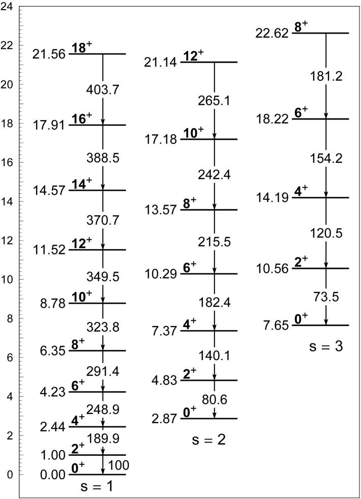
Figure 1: Energy levels of the ground state ($s=1$), $\beta_{1}$ ($s=2$), and $\beta_{2}$ ($s=3$) bands of X(3), normalized to the energy of the lowest excited state, $2_{1}^{+}$, together with intraband $B(E2)$ transition rates, normalized to the transition between the two lowest states, $B(E2;2_{1}^{+}\to 0_{1}^{+})$. Interband transitions are listed in Table 1. See Section 3 for further discussion.

The energy levels of the ground state band ($s=1$), as well as of the $\beta_{1}$ ($s=2$) and $\beta_{2}$ ($s=3$) bands, normalized to the energy of the lowest excited state, $2_{1}^{+}$, are shown in Fig. 1, together with intraband $B(E2)$ transition rates, normalized to the transition between the two lowest states, $B(E2;2_{1}^{+}\to 0_{1}^{+})$, while interband transitions are listed in Table 1.

The energy levels of the ground state band of X(3) are also shown in Fig. 2(a), where they are compared to the experimental data for ¹⁷²Os [20] (up to the point of bandcrossing) and ¹⁸⁶Pt [21]. In the same figure the ground state band of X(5), along with the experimental data for the $N=90$ isotones ¹⁵⁰Nd [22], ¹⁵²Sm [23], ¹⁵⁴Gd [24], and ¹⁵⁶Dy [25], which are considered as the best realizations of X(5) [5, 7, 8, 9, 10], are shown for comparison. The energy levels of the $\beta_{1}$-band for the same models and nuclei are shown in Fig. 2(b), while existing intraband $B(E2)$ transition rates for the ground state band are shown in Fig. 2(c). The following comments are now in place.

1) The ground state bands of ¹⁷²Os and ¹⁸⁶Pt are in very good agreement with the X(3) predictions, while the $\beta_{1}$-bands are a little lower. Similarly, the ground state bands of ¹⁵⁰Nd, ¹⁵²Sm, ¹⁵⁴Gd, and ¹⁵⁶Dy are in very good agreement with the X(5) predictions, while the $\beta_{1}$ bands beyond $L=4$ are much lower. This discrepancy is known to be fixed by considering [26] a potential with linear sloped walls instead of an infinite well potential. What occured rather unexpectedly is the fact that the $\beta_{1}$ bands of the $N=90$ isotones [the best experimental examples of X(5)] from $L=4$ upwards agree very well with the X(3) predictions. This could be interpreted as indication that the bandhead of the $\beta_{1}$ band is influenced by the presence of the $\gamma$ degree if freedom, but the excited levels of this band beyond $L=4$ are not influenced by it. Detailed measurements of intraband $B(E2)$ transition rates within the $\beta_{1}$-bands of these $N=90$ isotones could clarify this point.

2) Existing intraband $B(E2)$ transition rates for the ground state band of ¹⁷²Os (below the region influenced by the bandcrossing) are in good agreement with X(3), being quite higher than the ¹⁵⁰Nd, ¹⁵²Sm, and ¹⁵⁴Gd rates, as they should. [The $B(E2)$ rates of ¹⁵⁶Dy are known [9] to be in less good agreement with X(5), as also seen in Fig. 2(c).] However, more intraband and interband transitions (and with smaller error bars) are needed before final conclusions could be drawn. The same holds for ¹⁸⁶Pt, for which experimental information on B(E2)s is missing [21, 27]. The relative branching ratios known in ¹⁸⁶Pt [27] are given in Table 2, being in good agreement with the X(3) predictions.

The placement of the above mentioned nuclei in the symmetry triangle [28] of the Interacting Boson Model (IBM) [29] can be illuminating. All of the above mentioned N=90 isotones lie close to the phase coexistence and shape phase transition region of the IBM, with ¹⁵²Sm being located on the U(5)-SU(3) side of the triangle [30], while ¹⁵⁴Gd and ¹⁵⁶Dy gradually move towards the center of the triangle [31]. ¹⁷²Os [32] and ¹⁸⁶Pt [27] also appear near the center of the symmetry triangle and close to the transition region of the IBM.

It should be noticed that the critical character of ¹⁸⁶Pt is also supported by the criteria posed in Ref. [33]. In particular, a relatively abrupt change of the $R_{4}=E(4_{1}^{+})/E(2_{1}^{+})$ ratio occurs between ¹⁸⁶Pt and ¹⁸⁴Pt, as seen in the systematics presented in Ref. [32], while $0_{2}^{+}$ shows a minimum at ¹⁸⁶Pt, as seen in the systematics presented in Ref. [27], especially if the $0_{2}^{+}$ energies are normalized with respect to the $2_{1}^{+}$ state of each Pt isotope. Furthermore, ¹⁸⁶Pt is located at the point where the crossover of $0_{2}^{+}$ and $2_{\gamma}^{+}$ occurs, as seen in the systematics presented in Ref. [27].

4 Discussion

In summary, a $\gamma$-rigid (with $\gamma=0$) version of the X(5) model is constructed. The model is called X(3), since it is proved that only three variables occur in this case, the separation of variables being exact, while in the X(5) case approximate separation of the five variables occuring there is performed. The parameter free (up to overall scale factors) predictions of X(3) are found to be in good agreement with existing experimental data of ¹⁷²Os and ¹⁸⁶Pt, while a rather unexpected agreement of the $\beta_{1}$-bands of the X(5) nuclei ¹⁵⁰Nd, ¹⁵²Sm, ¹⁵⁴Gd, and ¹⁵⁶Dy to the X(3) predictions is observed. The need for further $B(E2)$ measurements in all of the above-mentioned nuclei is emphasized.

Table 1: Interband $B(E2;L_{i}\to L_{f})$ transition rates for the X(3) model, normalized to the one between the two lowest states, $B(E2;2_{1}^{+}\to 0_{1}^{+})$.

$L_{i}\to L_{f}$	X(3)	$L_{i}\to L_{f}$	X(3)	$L_{i}\to L_{f}$	X(3)
$0_{2}\to 2_{1}$	164.0
$2_{2}\to 4_{1}$	64.5	$2_{2}\to 2_{1}$	12.4	$2_{2}\to 0_{1}$	0.54
$4_{2}\to 6_{1}$	42.2	$4_{2}\to 4_{1}$	8.6	$4_{2}\to 2_{1}$	0.43
$6_{2}\to 8_{1}$	31.1	$6_{2}\to 6_{1}$	6.7	$6_{2}\to 4_{1}$	0.51
$8_{2}\to 10_{1}$	24.4	$8_{2}\to 8_{1}$	5.5	$8_{2}\to 6_{1}$	0.56
$10_{2}\to 12_{1}$	19.9	$10_{2}\to 10_{1}$	4.7	$10_{2}\to 8_{1}$	0.59
$12_{2}\to 14_{1}$	16.6	$12_{2}\to 12_{1}$	4.0	$12_{2}\to 10_{1}$	0.60
$14_{2}\to 16_{1}$	14.2	$14_{2}\to 14_{1}$	3.5	$14_{2}\to 12_{1}$	0.60
$16_{2}\to 18_{1}$	12.3	$16_{2}\to 16_{1}$	3.1	$16_{2}\to 14_{1}$	0.60
$18_{2}\to 20_{1}$	10.9	$18_{2}\to 18_{1}$	2.8	$18_{2}\to 16_{1}$	0.59
$20_{2}\to 22_{1}$	9.7	$20_{2}\to 20_{1}$	2.5	$20_{2}\to 18_{1}$	0.58
$0_{3}\to 2_{2}$	209.1
$2_{3}\to 4_{2}$	92.0	$2_{3}\to 2_{2}$	16.2	$2_{3}\to 0_{2}$	0.67
$4_{3}\to 6_{2}$	65.3	$4_{3}\to 4_{2}$	12.2	$4_{3}\to 2_{2}$	0.47
$6_{3}\to 8_{2}$	50.9	$6_{3}\to 6_{2}$	10.1	$6_{3}\to 4_{2}$	0.52
$8_{3}\to 10_{2}$	41.6	$8_{3}\to 8_{2}$	8.6	$8_{3}\to 6_{2}$	0.57
$10_{3}\to 12_{2}$	35.0	$10_{3}\to 10_{2}$	7.5	$10_{3}\to 8_{2}$	0.61
$12_{3}\to 14_{2}$	30.1	$12_{3}\to 12_{2}$	6.6	$12_{3}\to 10_{2}$	0.63
$14_{3}\to 16_{2}$	26.3	$14_{3}\to 14_{2}$	5.9	$14_{3}\to 12_{2}$	0.65
$16_{3}\to 18_{2}$	23.3	$16_{3}\to 16_{2}$	5.4	$16_{3}\to 14_{2}$	0.66
$18_{3}\to 20_{2}$	20.8	$18_{3}\to 18_{2}$	4.9	$18_{3}\to 16_{2}$	0.66
$20_{3}\to 22_{2}$	18.8	$20_{3}\to 20_{2}$	4.5	$20_{3}\to 18_{2}$	0.66

Table 2: Relative $B(E2)$ branching ratios for the X(3) model compared to existing exprerimental data [27] for ¹⁸⁶Pt.

$L_{i}\to L_{f}$	exp.	X(3)	$L_{i}\to L_{f}$	exp.	X(3)
$2_{2}\to 0_{2}$	100	100	$4_{2}\to 2_{2}$	100	100
$2_{2}\to 0_{1}$	8(1)	0.7	$4_{2}\to 2_{1}$	2.6(3)	0.3
$2_{2}\to 4_{1}$	68(7)	80	$4_{2}\to 4_{1}$	$<12$	6

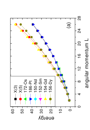
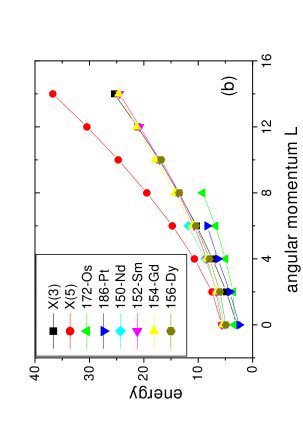
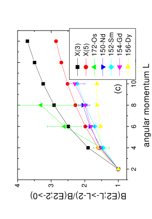
Figure 2: (a) Energy levels of the ground state bands of the X(3) and X(5) [2] models, compared to experimental data for ¹⁷²Os [20], ¹⁸⁶Pt [21], ¹⁵⁰Nd [22], ¹⁵²Sm [23], ¹⁵⁴Gd [24], and ¹⁵⁶Dy [25]. The levels of each band are normalized to the $2_{1}^{+}$ state. (b) Same for the $\beta_{1}$-bands, also normalized to the $2_{1}^{+}$ state. (c) Same for existing intraband $B(E2)$ transition rates within the ground state band, normalized to the $B(E2;2_{1}^{+}\to 0_{1}^{+})$ rate. The data for ¹⁵⁶Dy are taken from Ref. [9]. See Section 3 for further discussion.

References

- [1] F. Iachello, Phys. Rev. Lett. 85 (2000) 3580.
- [2] F. Iachello, Phys. Rev. Lett. 87 (2001) 052502.
- [3] R. F. Casten, N. V. Zamfir, Phys. Rev. Lett. 85 (2000) 3584.
- [4] R. M. Clark, et al., Phys. Rev. C 69 (2004) 064322.
- [5] R. F. Casten, N. V. Zamfir, Phys. Rev. Lett. 87 (2001) 052503.
- [6] R. M. Clark, et al., Phys. Rev. C 68 (2003) 037301.
- [7] R. Krücken, et al., Phys. Rev. Lett. 88 (2002) 232501.
- [8] D. Tonev, et al., Phys. Rev. C 69 (2004) 034334.
- [9] A. Dewald, et al., Eur. Phys. J. A 20 (2004) 173.
- [10] M. A. Caprio, et al., Phys. Rev. C 66 (2002) 054310.
- [11] A. Bohr, Mat. Fys. Medd. K. Dan. Vidensk. Selsk. 26, no. 14 (1952).
- [12] A. S. Davydov, A. A. Chaban, Nucl. Phys. 20 (1960) 499.
- [13] A. G. Sitenko, V. K. Tartakovskii, Lectures on the Theory of the Nucleus, Atomizdat, Moscow, 1972 (in Russian).
- [14] R. N. Zare, Angular Momentum, Wiley, New York, 1988.
- [15] A. S. Davydov, Theory of the Atomic Nucleus, Fizmatgiz, Moscow, 1958.
- [16] J. M. Eisenberg, W. Greiner, Nuclear Theory, Vol. I: Nuclear Models, North-Holland, Amsterdam, 1970.
- [17] A. O. Barut, R Raczka, Theory of Group Representations and Applications, World Scientific, Singapore, 1986.
- [18] D. Bonatsos, D. Lenis, N. Minkov, P. P. Raychev, P. A. Terziev, Phys. Rev. C 69 (2004) 044316.
- [19] D. R. Bès, Nucl. Phys. 10 (1959) 373.
- [20] B. Singh, Nucl. Data Sheets 75 (1995) 199.
- [21] C. M. Baglin, Nucl. Data Sheets 99 (2003) 1.
- [22] E. der Mateosian, J. K. Tuli, Nucl. Data Sheets 75 (1995) 827.
- [23] A. Artna-Cohen, Nucl. Data Sheets 79 (1996) 1.
- [24] C. W. Reich, R. G. Helmer, Nucl. Data Sheets 85 (1998) 171.
- [25] C. W. Reich, Nucl. Data Sheets 99 (2003) 753.
- [26] M. A. Caprio, Phys. Rev. C 69 (2004) 044307.
- [27] E. A. McCutchan, R. F. Casten, and N. V. Zamfir, Phys. Rev. C 71 (2005) 061301.
- [28] R. F. Casten, Nuclear Structure from a Simple Perspective, Oxford University Press, Oxford, 1990.
- [29] F. Iachello, A. Arima, The Interacting Boson Model, Cambridge University Press, Cambridge, 1987.
- [30] N. V. Zamfir, E. A. McCutchan, and R. F. Casten, Yad. Fiz. 67 (2004) 1856 [Phys. At. Nucl. 67 (2004) 1829].
- [31] E. A. McCutchan, N. V. Zamfir, and R. F. Casten, Phys. Rev. C 69 (2004) 063406.
- [32] E. A. McCutchan and N. V. Zamfir, Phys. Rev. C 71 (2005) 054306.
- [33] N. V. Zamfir, E. A. McCutchan, and R. F. Casten, in Nuclear Physics, Large and Small: International Conference on Microscopic Studies of Collective Phenomena, ed. R. Bijker, R. F. Casten, and A. Frank, AIP Conf. Proc. 726 (2004) 187.