Invisible nuclear system

Abstract

A consecutive formalism and analysis of exactly solvable radial reflectionless potentials with barriers, which in the spatial semiaxis of radial coordinate $r$ have one hole and one barrier, after which they fall down monotonously to zero with increasing of $r$, is presented. It has shown, that at their shape such potentials look qualitatively like radial scattering potentials in two-partial description of collision between particles and nuclei or radial decay potentials in the two-partial description of decay of compound spherical nuclear systems. An analysis shows, that the particle propagates without the smallest reflection and without change of an angle of motion (or tunneling) during its scattering inside the spherically symmetric field of the nucleus with such radial potential of interaction, i. e. the nuclear system with such interacting potential shows itself as invisible for the incident particle with any kinetic energy. An approach for construction of a hierarchy such reflectionless potentials is proposed, wave functions of the first potentials of this hierarchy are found.

PACS numbers: 11.30.Pb 03.65.-w, 12.60.Jv 03.65.Xp, 03.65.Fd,

Keywords: invisible nucleus, supersymmetry, exactly solvable model, reflectionless radial potentials, inverse power potentials, potentials of Gamov’s type, SUSY-hierarchy

1 Introduction

An interest to methods of supersymmetric quantum mechanics (SUSY QM) has been increasing every year. Initially constructed for a description of a symmetry between bosons and fermions in field theories, these methods during their development have formed completely independent section in quantum mechanics [1].

Today, the methods of SUSY QM are a powerful tool for calculation and analysis of spectral characteristics of quantum systems, they have shown as extremely effective in obtaining of new types of exactly solvable potentials and in analysis of their properties, in an evident explanation of such unusual phenomena from the point of view of common sense as a resonant tunneling, a reflectionless penetration (or an absolute transparency) of the potentials (differed from the resonant tunneling by that it exists in a whole energy spectrum, where a coefficient of reflection is not only minimal but equals to zero also), reinforcement of the barrier permeability and breaking of tunneling symmetry in opposite directions during the propagation of multiple of particles, absolute reflection for above-barrier energies, bound states in continuous energy spectra of systems [2, 3].

A number of papers has been increasing every year. Here, I should like to note a fine review [1], to note intensively developed methods of Nonlinear (also Polynomial, $N$-fold) supersymmetric quantum mechanics in [4, 5, 6, 7, 8, 9, 10]), methods of shape invariant potentials with different types of parameters transformations (for example, see [11, 12, 13, 14, 15, 16, 17, 18, 19]), methods of a description of self-similar potentials studied by Shabat [20] and Spiridonov [21, 22] and concerned with $q$-supersymmetry, methods of other types of potentials deformations and symmetries (for example, see [23]), non-stationary approaches for a description of properties and behavior of quantum systems [24]. One can note papers unified methods of supersymmetry with methods of inverse problem of quantum mechanics, and I should like to mention to nice monography [25] and reviews [3, 26] (with a literature list there). An essential progress has achieved in development of the methods of SUSY QM in spaces with different geometries [27], in non-commutative spaces [28]. Having a powerful and universal apparatus, now the methods of SUSY QM find their application in a number of tasks of field theories, in QCD, in development of different models of quantum gravity, cosmology and other.

However, in this paper I propose to pay attention into the reflectionless phenomenon in some types of spherical symmetric quantum systems (one note [4, 15, 25, 10, 29] in development of SUSY QM formalism for different scattering problems). We find out a new type of radial exactly solvable reflectionless potential, which in its shape has one hole and one barrier, after which it falls down monotonously to zero with increasing of radial coordinate $r$ [30]. Qualitatively, such potential looks like scattering potentials in two-partial description of collision between particle and spherically symmetric nucleus or decay potentials in the two-partial description of decay of compound spherical nuclear system. An analysis has shown that the particle propagates without the smallest reflection and without change of an angle of motion (or tunneling) in its scattering in the spherically symmetric field of the nucleus with such radial potential of interaction, i. e. the nuclear system with such potential shows itself as invisible for the incident particle with any kinetic energy. And this paper is devoted to an analysis of such radial reflection potentials.

2 SUSY-interdependence between spectral characteristics of potentials partners in the radial problem

2.1 Darboux transformations

Let’s consider a formalism of Darboux transformations in a problem about motion of a particle with mass $m$ in the spherically symmetric potential field (also see [4, 29]). The spherical symmetry of the potential allows to reduce this problem to the one-dimensional problem about the motion of this particle in the radial field $V(r)$, defined on the positive semiaxis of $r$, where wave function of such system looks like:

$$\psi(r,\theta,\varphi)=\displaystyle\frac{\chi_{nl}(r)}{r}Y_{lm}(\theta,\varphi),$$ (1)

and the radial Schrödinger equation has a form:

$$H\chi_{nl}(r)=-\displaystyle\frac{\hbar^{2}}{2m}\displaystyle\frac{d^{2}\chi_{nl}(r)}{dx^{2}}+\biggl{(}V_{n}(r)+\displaystyle\frac{l(l+1)\hbar^{2}}{2mr^{2}}\biggr{)}\chi_{nl}(r)=E_{n}\chi_{nl}(r)$$ (2)

and differs from the one-dimensional Schrödinger equation by a presence of a centrifugal term. One can reduce this equation to one-dimensional one by replacement:

$$\bar{V}_{n}(r)=V_{n}(r)+\displaystyle\frac{l(l+1)\hbar^{2}}{2mr^{2}}.$$ (3)

As in the one-dimensional case, one can introduce operators $A_{1}$ and $A_{1}^{+}$:

$$\begin{array}[]{ll}A_{1}=\displaystyle\frac{\hbar}{\sqrt{2m}}\displaystyle\frac{d}{dr}+W_{1}(r),&A_{1}^{+}=-\displaystyle\frac{\hbar}{\sqrt{2m}}\displaystyle\frac{d}{dr}+W_{1}(r),\end{array}$$ (4)

where $W_{1}(r)$ is a function, defined in the positive semiaxis $0\leq r<+\infty$ and continuous in it with an exception of some possible points of discontinuity. Then one can determine an interdependence between two hamiltonians of the propagation of the particle with mass $m$ in the fields $\bar{V}_{1}(r)$ and $\bar{V}_{2}(r)$:

$$\begin{array}[]{l}H_{1}=A_{1}^{+}A_{1}+C_{1}=-\displaystyle\frac{\hbar^{2}}{2m}\displaystyle\frac{d^{2}}{dr^{2}}+\bar{V}_{1}(r),\\ H_{2}=A_{1}A_{1}^{+}+C_{1}=-\displaystyle\frac{\hbar^{2}}{2m}\displaystyle\frac{d^{2}}{dr^{2}}+\bar{V}_{2}(r),\end{array}$$ (5)

where each potential is expressed through one function $W_{1}(r)$:

$$\begin{array}[]{ll}\bar{V}_{1}(r)=W_{1}^{2}(r)-\displaystyle\frac{\hbar}{\sqrt{2m}}\displaystyle\frac{dW_{1}(r)}{dr}+C_{1},&\bar{V}_{2}(r)=W_{1}^{2}(x)+\displaystyle\frac{\hbar}{\sqrt{2m}}\displaystyle\frac{dW_{1}(r)}{dr}+C_{1}.\end{array}$$ (6)

One can find:

$$\bar{V}_{2}(r)-\bar{V}_{1}(r)=V_{2}(r)-V_{1}(r)=2\displaystyle\frac{\hbar}{\sqrt{2m}}\displaystyle\frac{dW_{1}(r)}{dr}.$$ (7)

The determination of the potentials $V_{1}(r)$ and $V_{2}(r)$ of two quantum systems on the basis of one function $W_{1}(r)$ establishes the interdependence between spectral characteristics (spectra of energy, wave functions, S-matrixes) of these systems. We shall consider this interdependence, as the interdependence given by Darboux transformations in the radial problem, and we shall name $W_{1}(r)$ as superpotential, potentials $V_{1}(r)$ and $V_{2}(r)$ as supersymmetric potentials-partners.

Note, that there is a constant $C_{1}$ in the definition (2) of the hamiltonians of two quantum systems. If to choose $C_{1}=E^{(1)}_{0},E^{(2)}_{0}\neq E^{(1)}_{0}$ ($E^{(1)}_{0}$ and $E^{(2)}_{0}$ are the lowest levels of energy spectra of the first and second hamiltonians $H_{1}$ and $H_{2}$), then we obtain the most widely used construction two hamiltonians $H_{1}$ and $H_{2}$ in the one-dimensional case on the basis of the operators $A_{1}$ and $A_{1}^{+}$ (for example, see p. 287–289 in [1]). However, this case corresponds to bound states in the discrete regions of the energy spectra of two studied quantum systems. For study of scattering, decay or synthesis processes in the radial consideration usually we deal with unbound states with the continuous region of the energy spectra (with the lowest energy levels $C_{1}=E^{(1)}_{0}=E^{(2)}_{0}=0$) of quantum systems. Therefore, one need to use $C_{1}=0$ for obtaining the interdependence between the spectral characteristics of two systems on the basis of Darboux transformations (and we obtain a construction of hierarchy of potentials as in [30], see p. 443–445):

$$\begin{array}[]{l}H_{1}=A_{1}^{+}A_{1}=-\displaystyle\frac{\hbar^{2}}{2m}\displaystyle\frac{d^{2}}{dr^{2}}+\bar{V}_{1}(r),\\ H_{2}=A_{1}A_{1}^{+}=-\displaystyle\frac{\hbar^{2}}{2m}\displaystyle\frac{d^{2}}{dr^{2}}+\bar{V}_{2}(r).\end{array}$$ (8)

2.2 The interdependence between wave functions

We shall study two quantum systems, in each of which there is the scattering of the particle on the potential $V_{1}(r)$ or $V_{1}(r)$. Further, we shall not consider processes, concerned with loss of complete energy of systems (for example, dissipation, bremsstrahlung etc.). The energy spectra of these systems are continuous, and their lowest levels are zero. In accordence with (8), we write:

$$\begin{array}[]{l}H_{1}\chi^{(1)}_{k,l}=A_{1}^{+}A_{1}\chi^{(1)}_{k,l}=E^{(1)}_{k,l}\chi^{(1)}_{k,l},\\ H_{2}\chi^{(2)}_{k^{\prime},l^{\prime}}=A_{1}A_{1}^{+}\chi^{(2)}_{k^{\prime},l^{\prime}}=E^{(2)}_{k^{\prime},l^{\prime}}\chi^{(2)}_{k^{\prime},l^{\prime}},\end{array}$$ (9)

where $E^{(1)}_{k,l}$ and $E^{(2)}_{k^{\prime},l^{\prime}}$ are the energy levels of two systems with orbital quantum numbers $l$ and $l^{\prime}$, $\chi^{(1)}_{k,l}(x)$ and $\chi^{(2)}_{k^{\prime},l^{\prime}}(x)$ are the radial components of wave functions, concerned with these levels, $k=\displaystyle\frac{1}{\hbar}\sqrt{2mE^{(1)}_{k,l}}$ and $k^{\prime}=\displaystyle\frac{1}{\hbar}\sqrt{2mE^{(2)}_{k^{\prime},l^{\prime}}}$ are wave vectors corresponding to the levels $E^{(1)}_{k,l}$ and $E^{(2)}_{k^{\prime},l^{\prime}}$. From (9) we obtain:

$$H_{2}(A_{1}\chi^{(1)}_{k,l})=A_{1}A_{1}^{+}(A_{1}\chi^{(1)}_{k,l})=A_{1}(A_{1}^{+}A_{1}\chi^{(1)}_{k,l})=A_{1}(E^{(1)}_{k,l}\chi^{(1)}_{k,l})=E^{(1)}_{k,l}(A_{1}\chi^{(1)}_{k,l}).$$ (10)

We see, that the function $f(r)=A_{1}\chi^{(1)}_{k,l}(r)$ is the eigen-function of the operator $\hat{H}_{2}$ with quantum number $l$ to a constant factor, i. e. it represents the wave function $\chi^{(2)}_{k^{\prime},l}(r)$ of the hamiltonian $H_{2}$. The energy level $E^{(1)}_{k,l}$ must be the eigen-value of this operator exactly, i. e. it represents the energy level $E^{(2)}_{k^{\prime},l}$ of this hamiltonian. Here, new wave function and energy level have the same index ${k^{\prime}}$. One can write:

$$\begin{array}[]{lcr}A_{1}\chi^{(1)}_{k,l}(r)=N_{2}\chi^{(2)}_{k^{\prime},l}(r),&E^{(1)}_{k,l}=E^{(2)}_{k^{\prime},l},&N_{2}=const.\end{array}$$ (11)

Taking into account (9), one can write:

$$H_{1}(A_{1}^{+}\chi^{(2)}_{k^{\prime},l^{\prime}})=A_{1}^{+}A_{1}(A_{1}^{+}\chi^{(2)}_{k^{\prime},l^{\prime}})=A_{1}^{+}(A_{1}A_{1}^{+}\chi^{(2)}_{k^{\prime},l^{\prime}})=A_{1}^{+}(E^{(2)}_{k^{\prime},l^{\prime}}\chi^{(2)}_{k^{\prime},l^{\prime}})=E^{(2)}_{k^{\prime},l^{\prime}}(A_{1}^{+}\chi^{(2)}_{k^{\prime},l^{\prime}}).$$ (12)

and obtain:

$$\begin{array}[]{lcr}A_{1}^{+}\chi^{(2)}_{k^{\prime},l^{\prime}}(r)=N_{1}\chi^{(1)}_{k,l^{\prime}}(r),&E^{(2)}_{k^{\prime},l^{\prime}}=E^{(1)}_{k,l^{\prime}},&N_{1}=const.\end{array}$$ (13)

Thus, we obtain the following interdependences between the wave functions and the levels of the continuous energy spectra of two systems SUSY-partners in the radial problem:

$$\begin{array}[]{cccc}\chi^{(1)}_{k,l^{\prime}}(r)=\displaystyle\frac{1}{N_{1}}A_{1}^{+}\chi^{(2)}_{k^{\prime},l^{\prime}}(r),&\chi^{(2)}_{k^{\prime},l}(r)=\displaystyle\frac{1}{N_{2}}A_{1}\chi^{(1)}_{k,l}(r),&E^{(1)}_{k,l}=E^{(2)}_{k^{\prime},l},&E^{(1)}_{k,l^{\prime}}=E^{(2)}_{k^{\prime},l^{\prime}}.\end{array}$$ (14)

Darboux transformations establish the interdependence between the wave functions for the same energy levels of two systems. The coefficients $N_{1}$ and $N_{2}$ can be calculated from a normalization conditions for the wave functions (for the continuous energy spectra), and boundary condition are defined by scattering or decay process.

2.3 The interdependence between amplitudes of transittion and reflection

For scattering the radial superpotential $W_{1}(r)$, the potentials $V_{1}(r)$ and $V_{2}(r)$ are finite in the whole spatial region of their definition and in asymptotic they tend to zero:

$$\begin{array}[]{ll}W_{1}(r\to+\infty)=0,&V_{1}(r\to+\infty)=V_{2}(r\to+\infty)=0.\end{array}$$ (15)

Let’s find an interdependence between resonant and potential components of S-matrixes of these systems (for example, also see [4]).

One can describe the particle motion in the direction to zero inside the fields $V_{1}(r)$ and $V_{2}(r)$ with use of plane waves $e^{-ikr}$ (we assume, that the plane waves of both systems have the same wave vectors $k$). In spatial asymptotic regions we obtain transmitted waves $T_{1}(k)e^{ikx}$ and $T_{2}(k)e^{ikx}$, which are formed in result of total propagation (with possible tunneling) through the potentials and describe the resonant scattering of the particle on the potentials, and reflected waves $R_{1}(k)e^{ikx}$ and $R_{2}(k)e^{ikx}$, which are formed in result of reflection from the potentials and describe the potential scattering of the particle on the potentials. For each process of scattering one can write components of wave functions, which are formed in result of the transmission through the potential and the reflection from it:

$$\begin{array}[]{ll}\chi_{inc+ref}^{(1)}(k,r\to+\infty)=\bar{N}_{1}(e^{-ikr}+R_{1}e^{ikr}),&\chi_{tr}^{(1)}(k,r\to+\infty)\to\bar{N}_{1}T_{1}e^{ikr},\\ \chi_{inc+ref}^{(2)}(k,r\to+\infty)=\bar{N}_{2}(e^{-ikr}+R_{2}e^{ikr}),&\chi_{tr}^{(2)}(k,r\to+\infty)\to\bar{N}_{2}T_{2}e^{ikr},\end{array}$$ (16)

where the coefficients $\bar{N}_{1}$ and $\bar{N}_{2}$ can be found from the normalization conditions.

Using (16) for the wave functions in asymptotic region, taking into account the interdependence (14) between them and definitions (1) for the operators $A_{1}$ and $A_{1}^{+}$, we obtain:

$$\begin{array}[]{l}\bar{N}_{1}\biggl{(}e^{-ikr}+R_{1}e^{ikr}\biggr{)}=\displaystyle\frac{\bar{N}_{2}}{N_{1}}\displaystyle\frac{ik\hbar}{\sqrt{2m}}\biggl{(}e^{-ikr}-R_{2}e^{ikr}\biggr{)},\\ \bar{N}_{1}T_{1}e^{ikr}=-\displaystyle\frac{\bar{N}_{2}}{N_{1}}\displaystyle\frac{ik\hbar}{\sqrt{2m}}T_{2}e^{ikr}.\end{array}$$ (17)

These expressions are carried out only, if items with the same exponents are equal between themselves. We find:

$$\bar{N}_{1}=\displaystyle\frac{\bar{N}_{2}}{N_{1}}\displaystyle\frac{ik\hbar}{\sqrt{2m}}$$ (18)

and

$$\begin{array}[]{cc}R_{1}(k)=-R_{2}(k),&T_{1}(k)=-T_{2}(k).\end{array}$$ (19)

Exp. (19) establish the interdependence between the amplitudes of the transmission $T_{1}(k)$, $T_{2}(k)$ and the amplitudes of the reflection $R_{1}(k)$, $R_{2}(k)$ for the particle relatively two potentials. Squares of modules of the transmitted and reflected amplitudes represent the resonant and potential components of the S-matrixes for two systems. We see, that all these values do not depend on the normalized coefficients $N_{1}$, $N_{2}$, $\bar{N}_{1}$, $\bar{N}_{2}$.

One can introduce the matrix of scattering $S_{l}(k)$ for $l$-partial wave:

$$\chi_{nl}(r)\sim S_{l}(k)e^{ikr}-(-1)^{l}e^{-ikr}$$ (20)

and determine a phase shift $\delta_{l}(k)$:

$$e^{i\delta_{l}(k)}=S_{l}(k).$$ (21)

Then with taking into account (16), we find:

$$S_{l}(k)=(-1)^{l+1}(R_{l}(k)+T_{l}(k)).$$ (22)

One can see, how these partial components of the S-matrixes and the phases for two systems are interdependent (also see [1], p. 278–279):

$$\begin{array}[]{cc}S_{l}^{(1)}(k)=-S_{l}^{(2)}(k),&\delta_{l}^{(1)}(k)=\delta_{l}^{(2)}(k)+\pi/2.\end{array}$$ (23)

Let’s consider a spherically symmetric quantum system with the radial potential, to which a zero amplitude of the reflection $R(k)$ of the wave function corresponds. The particle during its scattering in this field propagates into a center without the smallest reflection by the field. In particular, such is a nul radial potential. We shall name such quantum systems and their radial potentials as reflectionless or absolutely transparent. Then from (19) one can see, that the potential-partner for the reflectionless potential is reflectionless also in that region, where it is finite. If such potential is finite on the whole region of its definition, then it is reflectionless completely (i. e. in standard definition of quantum mechanics). A series of the finite potentials of hierarchy, which contains the nul radial potential, should be reflectionless also. Using this simple idea and knowing a form of only one reflectionless potential, one can construct many new exactly solvable radial reflectionless potentials.

3 Spherically symmetric systems with absolute transparency

3.1 A radial reflectionless potentials with barriers

In [30] (see sec. 5.3.2, p. 459–462) an one-dimensional superpotential, defining a reflectionless potential which in semiaxis $0<x<+\infty$ has one hole, one barrier and then with increasing of $x$ falls down monotonously to zero in asymptotic region, had found. As this superpotential is obtained on the basis of interdependence between two one-dimensional hamiltonians with continuous energy spectra, one can use it in the problem about scattering of a particle in the spherically symmetric field with a barrier and with orbital quantum number $l=0$. In such case, we have:

$$\begin{array}[]{ll}W(r)=\displaystyle\frac{2\beta-\alpha}{f(\bar{r})}-\displaystyle\frac{\beta}{\bar{r}},&\mbox{ }2\beta\neq\alpha,\end{array}$$ (24)

where

$$f(\bar{r})=C(2\beta-\alpha)\bar{r}^{2\beta/\alpha}+\bar{r}.$$ (25)

Here $\bar{r}=r+r_{0}$, $\beta$ and $C$ are arbitrary real positive constants, $r_{0}$ is a positive number close to zero, and a designation $\alpha=\displaystyle\frac{\hbar}{\sqrt{2m}}$ is introduced. This superpotential is defined on the positive semiaxis of $r$ (at $r>r_{0}$).

Let’s find potentials-partners for the superpotential (24). In accordance with (6), we obtain:

$$\begin{array}[]{lcl}V_{1,2}(r)&=&\displaystyle\frac{(2\beta-\alpha)^{2}}{f^{2}(\bar{r})}-\displaystyle\frac{2\beta(2\beta-\alpha)}{\bar{r}f(\bar{r})}+\displaystyle\frac{\beta^{2}}{\bar{r}^{2}}\pm\\ &\pm&\Biggl{(}\displaystyle\frac{(2\beta-\alpha)^{2}}{f^{2}(\bar{r})}-\displaystyle\frac{2\beta(2\beta-\alpha)}{\bar{r}f(\bar{r})}+\displaystyle\frac{\alpha\beta}{\bar{r}^{2}}\Biggr{)}\end{array}$$ (26)

or

$$\begin{array}[]{lcl}V_{1}(r)&=&\displaystyle\frac{\beta(\beta-\alpha)}{\bar{r}^{2}},\\ V_{2}(r)&=&2\displaystyle\frac{(2\beta-\alpha)^{2}}{f^{2}(\bar{r})}-\displaystyle\frac{4\beta(2\beta-\alpha)}{\bar{r}f(\bar{r})}+\displaystyle\frac{\beta(\beta+\alpha)}{\bar{r}^{2}}.\end{array}$$ (27)

From (27) one can see that at $\beta=\alpha$ the first potential $V_{1}(r)$ obtains zero value and, therefore, it becomes reflectionless. Then, according to (19), if the second potential $V_{2}(r)$ is finite in a whole region of its definition, then it should be reflectionless also. At $\beta=\alpha$ we obtain:

$$V_{2}(r)=\displaystyle\frac{2\alpha^{2}}{\biggl{(}r+r_{0}+\displaystyle\frac{1}{C\alpha}\biggr{)}^{2}}.$$ (28)

We see, that this potential is finite in the whole region of its definition at any values of the parameters $C>0$ and $r_{0}\geq 0$. Thus, we have obtained the reflectionless potential of the inverse power type with a shift to the left, which is defined on the whole positive semiaxis of $r$ (including $r=0$ and $r_{0}=0$).

In accordance with [30] (see p. 452–455, sec. 5.1.2), one can construct a hierarchy of the inverse power potentials, and a general solution of the potential with arbitrary number $n$ can be written down so:

$$\begin{array}[]{ll}V_{n}(r)=\displaystyle\frac{\gamma_{n}\alpha^{2}}{\bar{r}^{2}},&\gamma_{n\pm 1}=1+\gamma_{n}\pm\sqrt{4\gamma_{n}+1}.\end{array}$$ (29)

If to require, that the first potential $V_{1}(r)$ in this hierarchy must be constant (i. e. at $\gamma_{1}=0$ and $n=1$), then all hierarchy of the inverse power potentials (29) becomes the hierarchy of the reflectionless inverse power potentials, and the solution (28) becomes the general solution for the reflectionless inverse power potential. Note, that when the hierarchy of the inverse power potentials becomes reflectionless, then the coefficients $\gamma_{n}$ become integer numbers. We write its first values:

$$\gamma_{n}=0,2,6,12,20,30,42...$$ (30)

Now, if to calculate $\beta_{n}$ for given $\gamma_{n}$ with number $n$ from (30) from the following condition:

$$\beta_{n}(\beta_{n}-\alpha)=\gamma_{n}\alpha^{2},$$ (31)

then the first potential $V_{1}(r)$ from (27) becomes reflectionless inverse power potential (at $\beta=\beta_{n}$). The second potential $V_{2}(r)$ from (27) is finite in the whole region of its definition (including $r=0$) and should be reflectionless also, however it is not inverse power potential. So, substituting the coefficients $\gamma_{n}$ with other numbers $n$ into the second expression (27) for the potential $V_{2}(r)$, one can construct the whole hierarchy of the radial reflectionless potentials of this new type.

In Fig. 1 the potential $V_{2}(r)$ for the chosen values of the parameters $C$ and $\gamma_{n}$ is shown. From here one can see, that such potential has one hole and one barrier, after which it falls down monotonously to zero with increasing of the radial coordinate $r$.

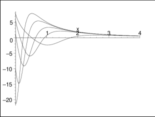
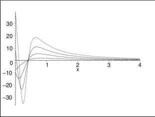
Figure 1: A dependence of the radial potential $V_{2}(r)$ on $C$ and $\gamma_{n}$: (a) the barrier maximum and the hole minimum of this potential are changed along the axis $r$ at the change of $C$ (at $C=0.01,0.1,0.3,1.0,2.5$, $\gamma_{n}=6$, $r_{0}=0.5$); (b) the barrier maximum of this potential practically does not changed along the axis $r$ at the change of $\gamma_{n}$ (at $C=1$, $\gamma_{n}=2,6,12,20$, $r_{0}=0.5$).

In its behavior such potential looks qualitatively like radial potentials with barriers used in theory of nuclear collisions for a description of scattering of particles on spherical nuclei, and for a description of decay and synthesis of nuclei of a spherical type also. This potential is reflectionless, if the parameter $\gamma_{n}$ has discrete values from the sequence (30). For any reflectionless potential with given $\gamma_{n}$ one can displace continuously its barrier and hole along an axis $r$ by use of the parameter $C$. Such deformation of the shape of the reflectionless potential is shown in Fig. 2.

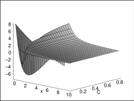
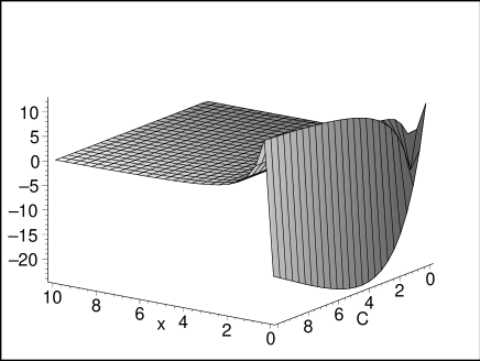
Figure 2: The reflectionless radial exactly solvable potential $V_{2}(r)$ with the barrier. Continuous change of its shape at variation of $C$ ($\gamma_{n}=6$, $r_{0}=0.5$)

3.2 An analysis of wave functions

3.2.1 Wave functions for the reflectionless inverse power potential

Let’s find a radial wave function describing the scattering of the particle on the inverse power reflectionless potential (28) at $l=0$. For the potential $V_{1}(r)$ with zero value of (27) one can write its radial wave function (for arbitrary energy level concerned with wave vector $k$) at $l=0$ by such a way (at $\beta=\alpha$):

$$\chi_{l=0}^{(1)}(k,r)=\bar{N}_{1}(e^{-ikr}-S_{l=0}^{(1)}e^{ikr}).$$ (32)

Then, one can find a radial wave function at $l=0$ for the reflectionless potential $V_{2}(r)$ of (28) (for the energy level corresponding to the wave vector $k$) on the basis of the second expression of (14). Taking into account (4) and (23), we obtain:

$$\begin{array}[]{lcl}\chi_{l=0}^{(2)}(k,r)&=&\displaystyle\frac{1}{N_{2}}A_{1}\chi_{l=0}^{(1)}(k,r)=\displaystyle\frac{\bar{N}_{1}}{N_{2}}\biggl{(}\alpha\displaystyle\frac{d}{dr}+W(r)\biggr{)}\Bigl{(}e^{-ikr}-S_{l=0}^{(1)}e^{ikr}\Bigl{)}=\\ &=&\chi_{l=0}^{(-)}(k,r)-S_{l=0}^{(2)}\chi_{l=0}^{(+)}(k,r),\end{array}$$ (33)

where

$$\chi_{l=0}^{(\pm)}(k,r)=\bar{N}_{2}\biggl{(}1\mp\displaystyle\frac{iW(r)}{k\alpha}\biggr{)}e^{\pm ikr}$$ (34)

and

$$\bar{N}_{2}=i\displaystyle\frac{\bar{N}_{1}}{k\alpha N_{2}}$$ (35)

In accordance with main statements of quantum mechanics, for applying such form of the radial wave function to the description of scattering of the particle in the field of the potential $V_{2}(r)$, it needs to achieve a boundary requirement $\chi_{l=0}^{(2)}(k,r)\to 0$ at $r\to 0$, which gives a finiteness of the wave function (1) at $r=0$ (and $S_{l=0}^{(2)}$ must have finite values and be not zero). One can see from (33), that it is fulfilled only in case ($W(r)$ is real):

$$\begin{array}[]{lcl}Re(S_{l=0}^{(2)})=\displaystyle\frac{k^{2}\alpha^{2}-W^{2}(0)}{k^{2}\alpha^{2}+W^{2}(0)},&Im(S_{l=0}^{(2)})=\displaystyle\frac{2W(0)k\alpha}{k^{2}\alpha^{2}+W^{2}(0)},\end{array}$$ (36)

where

$$W(0)=-\displaystyle\frac{\alpha}{r_{0}+\displaystyle\frac{1}{C\alpha}}.$$ (37)

For the partial components of the S-matrix the following property $|S_{l=0}|^{2}=1$ is fulfilled also. In limit $r\to 0$ we obtain the following expression for the radial wave function:

$$\chi_{l=0}^{(2)}(k,r)=\bar{N}_{2}\biggl{(}1+\displaystyle\frac{iW(0)}{k\alpha}\biggr{)}\biggl{(}e^{-ikr}-S_{l=0}^{(2)}\displaystyle\frac{k\alpha-iW(0)}{k\alpha+iW(0)}e^{ikr}\biggl{)},$$ (38)

which in its form coincides with Exp. (32) for the wave function for the potential $V_{1}(r)$ from (27) with zero value.

In Fig. 3 real and imaginary parts of the wave function near to the point $r=0$ are shown (here the starting formulas (33)–(34) are taken). From Fig. 3 (a, b) one can see a deformation of the imaginary part of this wave function with change of the wave vector $k$ and the parameter $C$. The real part of the wave function in its behavior looks like the imaginary part (see Fig. 3 (c)). Here, one can see also that at such choice of the real and imaginary parts of the partial components of the S-matrix the wave function leaves from its zero value at $r=0$.

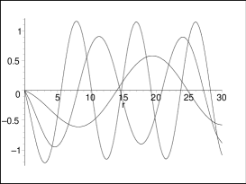
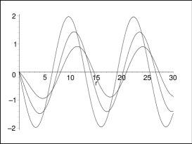
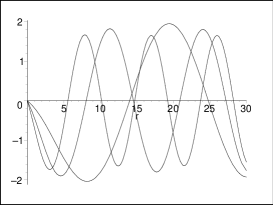
Figure 3: The dependence of the radial wave function (33) from the wave vector $k$ and the parameter $C$ (the values of $\alpha=1$, $r_{0}=0$, $\bar{N}_{2}=1$ are chosen): (a) a displacement of peaks of the imaginary part of the wave function along the semiaxis of $r$ is shown with change of the wave vector $k$ (at $k=0.3,0.5,0.7$, $C=1$); (b) the displacement of the peaks of the imaginary part of the wave function along the semiaxis of $r$ is shown with change of the parameter $C$ (at $C=0.1,0.5,1.0$, $k=0.5$); (c) the real part of the wave function is shown (at $k=0.3,0.5,0.7$, $C=1$)

In Fig. 4 an evident picture of behavior of the imaginary part of the wave function close to point $r=0$ with continuous change of the wave vector $k$ and the parameter $C$ is shown.

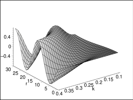
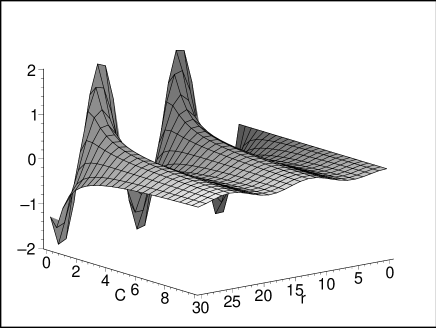
Figure 4: Behavior of the imaginary part of the wave function (33) depending on the wave vector $k$ and the parameter $C$ (the values $\alpha=1$, $r_{0}=0$, $\bar{N}_{2}=1$) are used): (a) dependence on the wave vector $k$ (at $C=1$); (b) dependence on the parameter $C$ (at $k=0.5$)

Note, that according to (23), the condition (36) can bring to not zero values of the radial wave function $\chi_{l=0}^{(1)}(k,r)$ at $r\to 0$ and can give discontinuity of the total wave function. However, a variation of the phase of $S_{l=0}^{(1)}$ does not change the form of the potential $V_{1}(r)$, which remains zero and reflectionless. In other words, the reflectionless potential $V_{1}(r)$ allows an arbitrariness in a choice of boundary conditions for the wave function at point $r=0$, and the chosen boundary conditions define the shape of the total wave function and a process proceeding in the field of the potential $V_{1}(r)$. There is a similar situation for the potential $V_{2}(r)$, which remains reflectionless with the variation of the S-matrix phase.

Now let’s analyze the form of the wave function (33) in asymptotic region. According to (24), $W(r)\to 0$ at $r\to+\infty$ and we obtain:

$$\chi_{l=0}^{(2)}(k,r)=\bar{N}_{2}\biggl{(}e^{-ikr}-S_{l=0}^{(2)}e^{ikr}\biggr{)}.$$ (39)

One can see, that two components $\chi_{l=0}^{(\pm)}(k,r)$ in (33) represent convergent and divergent waves, that can be useful for analysis of propagation of the particle in the field $V_{2}(r)$. Thus, we have found an exact analytical division of the total radial wave function into its convergent and divergent components (as for regular and singular Coulomb functions for the known Coulomb potential) in the description of scattering of the particle in the inverse power potential (28).

If for the convergent and divergent waves to define radial flows as:

$$j^{\pm}(k,r)=\displaystyle\frac{i\hbar}{2m}\biggl{(}\chi_{l=0}^{(\pm)}(k,r)\displaystyle\frac{d\chi_{l=0}^{(\pm),*}(k,r)}{dr}-\chi_{l=0}^{(\pm),*}(k,r)\displaystyle\frac{d\chi_{l=0}^{(\pm)}(k,r)}{dr}\biggr{)},$$ (40)

then for both waves we obtain coincided absolute values of their flows:

$$j^{\pm}(k,r)=\pm\displaystyle\frac{\hbar k}{m}|\bar{N}_{2}|^{2}.$$ (41)

We see, that the flows do not vary in dependence on $r$, and this gives a fulfillment of a conservation law for the flows from each wave and the total flow. Therefore, the convergent wave $\chi_{l=0}^{(-)}(k,r)$ propagates into the center without the smallest reflection by the field, because it is defined and is continuous on the whole region of the definition of the potential (28) and it forms the constant radial flow $j^{-}(r)$. Now we can tell with confidence, that the inverse power radial potential (28), for which we have found the radial wave function (33)–(35) for scattering, is reflectionless at $l=0$.

Further, one can find the radial wave functions at $l\neq 0$ on the basis of the same analysis, if for the radial wave function (32) for the potential with zero value to use spherical Hankel functions instead of factors $\exp{(\pm ikr)}$.

3.2.2 Wave functions for the reflectionless potential with the barrier

One can use Exp. (27) for calculation of a new reflectionless potential $V_{2}(r)$ with a barrier on the basis of the known reflectionless inverse power potential $V_{1}(r)$. Let’s assume, that these potentials are connected with one superpotential $W_{2}(r)$. Let’s consider the wave function for the reflectionless inverse power potential $V_{1}(r)$ at $l=0$ in the form:

$$\chi_{l=0}^{(1)}(k,r)=\bar{N}_{1}\Bigl{(}f^{-}(r)e^{-ikr}-S_{l=0}^{(1)}f^{+}(r)e^{ikr}\Bigr{)}.$$ (42)

Then the radial wave function at $l=0$ for the reflectionless potential $V_{2}(r)$ with the barrier can be found on the basis of the second expression of (14). Taking into account (4) and (23), we obtain:

$$\begin{array}[]{lcl}\chi_{l=0}^{(2)}(k,r)&=&\displaystyle\frac{\bar{N}_{1}}{N_{2}}\biggl{(}\alpha\displaystyle\frac{d}{dr}+W_{2}(r)\biggr{)}\Bigl{(}f^{-}(r)e^{-ikr}-S_{l=0}^{(1)}f^{+}(r)e^{ikr}\Bigr{)}=\\ &=&\displaystyle\frac{\bar{N}_{1}}{N_{2}}\biggl{[}\biggl{(}\alpha\displaystyle\frac{df^{-}(r)}{dr}-ik\alpha f^{-}(r)+W_{2}(r)f^{-}(r)\biggr{)}e^{-ikr}-\\ &-&S_{l=0}^{(2)}\biggl{(}\alpha\displaystyle\frac{df^{+}(r)}{dr}+ik\alpha f^{+}(r)+W_{2}(r)f^{+}(r)\biggr{)}e^{ikr}\biggr{]}.\end{array}$$ (43)

In this expression one can see the division of the total radial wave function into the convergent and divergent components, that can be interesting in analysis of scattering (with possible tunneling) of the particle in the field of the reflectionless potential $V_{2}(r)$ with the barrier.

So, if to use the potential (28) as the first reflectionless inverse power potential, then we find:

$$\beta_{2}=2\alpha$$ (44)

and

$$\begin{array}[]{lcl}f^{\pm}(r)=1\pm\displaystyle\frac{i}{k\biggl{(}\bar{r}+\displaystyle\frac{1}{C\alpha}\biggr{)}},&\displaystyle\frac{df^{\pm}(r)}{dr}=\mp\displaystyle\frac{i}{k\biggl{(}\bar{r}+\displaystyle\frac{1}{C\alpha}\biggr{)}^{2}},&W_{2}(r)=\displaystyle\frac{\alpha}{\bar{r}}\displaystyle\frac{1-6C\alpha\bar{r}^{3}}{1+3C\alpha\bar{r}^{3}}.\end{array}$$ (45)

Substituting these expressions into (43), one can find the total radial wave function for the reflectionless potential with the barrier. The value of the partial component of the S-matrix $S_{l=0}^{(2)}$ can be found from a boundary condition of this wave function at point $r=0$, as it was made in the previous paragraph for the inverse power reflectionless potential (28).

4 Conclusions

In finishing we note main conclusion and new results.

• The new exactly solvable radial reflectionless potential with barrier, which in the spatial semiaxis of radial coordinate $r$ has one hole and one barrier, after which it falls down monotonously to zero with increasing of $r$, is proposed. It has shown, that at its shape such potential looks qualitatively like radial scattering potentials in two-partial description of collision between particles and nuclei or radial decay potentials in the two-partial description of decay of compound spherical nuclear systems.

• The found reflectionless potential with the barrier depends on parameters $\gamma_{n}$ and $C$. One can deform the shape of this potential: by discrete values of $\gamma_{n}$ (from the sequence (30)) and by continuous values of $C$. The parameter $\gamma_{n}$ at its variation does not displace visibly a maximum of the barrier and a minimum of the hole along the semiaxis $r$, but it changes their absolute values. The parameter $C$ allows to displace continuously both the barrier maximum and the hole minimum.

• A new approach for construction of a hierarchy of the radial reflectionless potentials with barriers is proposed.

• An exact analytical form for the total radial wave function, its convergent and divergent components (as for regular and singular Coulomb functions for the known Coulomb potential) has found in the description of scattering of a particle in the field of the inverse power reflectionless potential and in the field of the reflectionless potential with the barrier (at $\beta=2\alpha$).

• It has shown for the inverse power potential, that the radial flows for the convergent and divergent components of the radial wave function are constant on the whole semiaxis of $r$, have opposite directions and coincide by absolute values. This proves the reflectionless property of the inverse power potential (with a possible tunneling near the point $r=0$) on the whole semiaxis $r$. Such analysis is applicable for the found potential with the barrier also.

The analysis has shown, that any selected region of the reflectionless potential with the barrier (with take into account both the barrier region, and the small vicinity near $r=0$) does not influence on the propagation of the particle. During scattering in the spherically symmetric field with such radial potential, the particle propagates through it without the smallest reflection and without any change of angle of direction of its motion (or tunneling). One can conclude, that the found radial potential with the barrier is reflectionless for the propagation of the particle with any kinetic energy. If to use it for the two-partial description of the scattering of the particle on the nucleus with the spherical shape, then one can conclude, that such nucleus shows itself as invisible for the incident particle.

References

- [1] Cooper F., Khare A. and Sukhatme U., Supersymmetry and quantum mechanics, Physics Reports, 1995, V. 251, 267–385; hep-th/9405029.
- [2] Chabanov V. M. and Zakhariev B. N., Absolutely transparent multichannel systems. Unexpected peculiarities, Physics Letters B, 1993, V. 319, N. 1–3, 13–15.
- [3] Zakhariev B. N. and Chabanov V. M., Qualitative theory of control of spectra, scattering, decays (Quantum intuition lessons), Physics of elementary particles and atomic nuclei, 1994, V. 25, Iss. 6, 1561–1597 — [in Russian].
- [4] Andrianov A. A., Cannata F., Dedonder J.-P. and Ioffe M. V., Second order derivative supersymmetry and scattering problem, International Journal of Modern Physics A, 1995, V. 10, 2683–2702; hep-th/9404061.
- [5] Aoyama H., Sato M. and Tanaka T., -fold supersymmetry in quantum mechanics — general formalism, Nuclear Physics B, 2001, V. 619, 105–127; quant-ph/0106037.
- [6] Sato M. and Tanaka T., -fold supersymmetry in quantum mechanics — analyses of particular models, Journal of Mathem. Physics, 2002, V. 43, 3484–3510; hep-th/0109179.
- [7] Gonzalez-Lopez A. and Tanaka T., A new family of -fold supersymmetry: type B, Physical Letters B, 2004, V. 586, 117–124; hep-th/0307094.
- [8] Andrianov A. A. and Sokolov A. V., Nonlinear supersymmetry in Quantum Mechanics: algebraic properties and differential representation, Nuclear Physics B, 2003, V. 660, 25–50; hep-th/0301062.
- [9] Andrianov A. A. and Cannata F., Nonlinear supersymmetry for spectral design in quantum mechanics, Journal of Physics A, 2004, V. 37, 10297–10323; hep-th/0407077.
- [10] Niederle J. and Nikitin A. G., Extended SUSY with central charges in quantum mechanics, in Proceedings of Institute of mathematics, Kyiv, 2002, V. 43, Part 2, 497–507.
- [11] Gendenshtein L., Derivation of exact spectra of the Schrodinger equation by means of supersymmetry, JETP Lett., 1983, V. 38, 356–359.
- [12] Dutt R., Khare A. and Sukhatme U. P., Exactness of supersymmetric WKB spectra for shape invariant potentials, Physics Letters B, 1986, V. 181, 295.
- [13] Cooper F., Ginocchio J. N. and Khare A., Relationship between supersymmetry and solvable potentials, Physical Review D, 1987, V. 36, N. 8, 2458–2473.
- [14] Dutt R., Khare A. and Sukhatme U., Supersymmetry, shape invariance and exactly solvable potentials, American Journal of Physics, 1988, V. 56, 163–168.
- [15] Khare A. and Sukhatme U. P., Scattering amplitudes for supersymmetric shape invariant potentials by operator methods, Journal of Physics A: Mathematical and General 1988, V. 21, L501–L508.
- [16] Khare A. and Sukhatme U. P., New shape invariant potentials in supersymmetric quantum mechanics, Journal of Physics A: Mathematical and General, 1993, V. 26, L901–L904; hep-th/9212147.
- [17] Barclay D. T., Dutt R., Gangopadhyaya A., Khare A., Pagnamenta A. and Sukhatme U., New exactly solvable Hamiltonians: shape invariance and self-similarity, Physical Review A, 1993, V. A48, 2786–2797; hep-ph/9304313.
- [18] Balantekin A. B., Algebraic approach to shape invariance, Physical Review A, 1998, V. A57, 4188–4191; quant-ph/9712018.
- [19] Andrianov A. A., Cannata F., Ioffe M. V. and Nishnianidze D. N., Systems with higher-order shape invariance: spectral and algebraic properties, Physics Letters A, 2000, V. 266, 341–349; quant-ph/9902057.
- [20] Shabat A., Inverse Problems, 1992, V. 8, 303.
- [21] Spiridonov V., Exactly solvable potentials and quantum algebras, Physical Review Letters, 1992, V. 69, N. 3, 398–401; hep-th/9112075.
- [22] Spiridonov V., The factorization method, self-similar potentials and quantum algebras, Lecture at the NATO Advanced Study Institute on special functions, “Special Functions 2000: Current Perspective and Future Directions” (Kluwer Academic Publishers, Dordrecht, Tempe, Arizona, 29 May - 9 Jun 2000) Editors J. Bustoz, M.E.H. Ismail and S.K. Suslov, 2001, 335–364. hep-th/0302046.
- [23] Gómez-Ullate D. , Kamran N. and Milson R., The inverse Darboux transformation and exactly solvable deformations of shape-invariant potentials, Journal of Physics A: Mathematical and General, 2004, V. 37, N. 5–6, 1780–1804; quant-ph/0308062.
- [24] Samsonov B. F., Time-dependent supersymmetry and parasupersymmetry in quantum mechanics, in Proceedings of Institute of mathematics, Kyiv, 2002, V. 43, Part 2, 520–529.
- [25] Chadan K. and Sabatier P. C., Inverse problems in quantum scattering theory, Springer-verlag, New York, 1977, 344 p.
- [26] Zakhariev B. N. and Chabanov V. M., On the qualitative theory of elementary transformations of one- and multicannel quantum systems in the inverse problem approach, Physics of elementary particles and atomic nuclei, 1999, V. 30, Iss. 2, 277–320 — [in Russian].
- [27] Samsonov B. F., Darboux transformation of coherent states for a Lobachevski plane, Russ. Phys. Journ., 1997, V. 40, 848–855.
- [28] Ghosh P. K., Supersymmetric quantum mechanics on non-commutative space, The European Physical Journal C, 2005, 9 p..
- [29] Bagrov V. G., Samsonov B. F. and Shekoyan L. A. N-order Darboux transformation and a spectral problem on semiaxis, Russ. Phys. Journ., 1997, V. 40, 848–855; quant-ph/9804032.
- [30] Maydanyuk S. P., SUSY-hierarhy of one-dimensional reflectionless potentials, Annals of Physics, 2005, V. 316, N. 2, 440–465; hep-th/0407237.