Precise numerical results for limit cycles
in the quantum three-body problem

Abstract

The study of the three-body problem with short-range attractive two-body forces has a rich history going back to the 1930’s. Recent applications of effective field theory methods to atomic and nuclear physics have produced a much improved understanding of this problem, and we elucidate some of the issues using renormalization group ideas applied to precise nonperturbative calculations. These calculations provide 11-12 digits of precision for the binding energies in the infinite cutoff limit. The method starts with this limit as an approximation to an effective theory and allows cutoff dependence to be systematically computed as an expansion in powers of inverse cutoffs and logarithms of the cutoff. Renormalization of three-body bound states requires a short range three-body interaction, with a coupling that is governed by a precisely mapped limit cycle of the renormalization group. Additional three-body irrelevant interactions must be determined to control subleading dependence on the cutoff and this control is essential for an effective field theory since the continuum limit is not likely to match physical systems (e.g., few-nucleon bound and scattering states at low energy). Leading order calculations precise to 11-12 digits allow clear identification of subleading corrections, but these corrections have not been computed.

I Introduction

It has been known since the 1930’s that a non-relativistic three-body system with short-range two-body potentials has a peculiar behavior, with a binding energy that is unexpectedly large. In fact the binding energy becomes infinite if the range of the attractive two-body potential is shrunk to zero Tho35 . For over 30 years it has also been known that the three-body bound state spectrum exhibits an Efimov effect Efi70 ; Efi71 . There are an increasing number of three-body bound states as the two-body effective range is reduced or as a high momentum cutoff is increased, as long as the two-body bound state energy is held fixed. For sufficiently large cutoff, $\Lambda$, the ratio of the energies of two successive three-body bound states approaches an analytically fixed limit of approximately 515.035 for energies much deeper than the two-body binding energy Albe81 .

More recently, Bedaque, Hammer, and van Kolck have shown that the short-range three-body problem is renormalizable, but only if a point-like three-body interaction is added BHK99 ; BHK99b ; BHK00 . The dimensionless version of the three-body coupling strength [which they denote by $H(\Lambda)$ but we denote by $G_{3}(\Lambda)]$ has an unexpected dependence on $\Lambda$, namely $G_{3}(\Lambda)$ has a periodic dependence on $\ln\Lambda$. In each period the value of $G_{3}(\Lambda)$ steadily increases until it reaches plus infinity. It jumps to minus infinity and then steadily increases again. This peculiar behavior provides a rare example of a renormalization group limit cycle Wil00 ; Wil71 ; Glazek02 , with the exciting possibility that scaling behavior near a limit cycle might be studied experimentally Bra04 .

Unfortunately, the two experimental candidates to be Efimov-like, namely the triton and the atomic helium trimer, do not exhibit the infinite set of shallow Efimov states because that would require the nucleon-nucleon S-waves or helium dimer systems to have a bound state precisely at threshold Efi70 ; Efi71 . This is not the case experimentally. The reality is that the triton has only one bound state. In the case of the helium trimer numerical calculations for realistic potential models indicate that the trimer has two bound states. These departures from the infinite Efimov limit raises the question: what are the corrections to the Efimov limit in the three-body system when the two-body system does not have a bound state precisely at threshold? How large are the corrections in the case that there are only one or two Efimov states rather than an infinite number?

Ideally, one would answer this question for the most plausible three-body Hamiltonians that have been proposed for describing the triton or the helium trimer [see refs. in Bra04 ]. But realistic three-body Hamiltonians are very demanding to study. Their three-body eigenfunctions are functions of three variables in the simplest case (S-states), making both analytical and numerical analysis exceptionally difficult (although far from impossible). Fortunately, it is possible to formulate a cutoff form of a two-body zero range potential (a delta-function potential $V({\bf r})=g\delta^{3}({\bf r})$) in which the Schrödinger equation wave function can be expressed exactly in terms of a reduced wave function $\phi(r)$ that depends only on one radial variable rather than three variables. The Schrödinger equation itself becomes a one-dimensional integral equation for $\phi(r)$ and the energy eigenvalue $E$ (although with auxiliary functions that involve integrals over known functions).

The one-dimensional integral equation can be solved numerically and quickly to machine precision (around 12 decimal places in our calculations) on a PC, although achieving this high precision involves careful attention to details of how the reduced wave function and the integral equation are discretized. High numerical accuracy is invaluable for testing the validity of analytic but approximate formulae for the corrections to the Efimov limit.

The integral equation will be formulated and solved for the Fourier transform $\Phi(p)$ of the reduced wave function. Uniformly valid expansions (e.g., with uniform convergence to the exact solution over the entire range of momenta) are employed to systematically dissect the bound state equation so that high-momentum behavior is isolated analytically. Low, intermediate and high momentum scales in the bound-state wavefunction are isolated by defining approximations to the full wavefunction that are valid in each of these three regions, and then showing that these can be assembled to produce an approximation that is valid for all momenta. The wave-functions valid at low and high momenta “communicate” through a single phase found in an analytic solution for the intermediate momenta approximation, all to leading order.

The outcome of the analytic and numerical analysis of this article is that Efimov three-body bound states have energy eigenvalues $B_{3}^{(n)}$ whose infinite cutoff limits can be precisely computed, and a simple renormalization group analysis suggests the leading corrections are of order $\sqrt{B_{2}}~{}{\rm ln}(\Lambda)/\Lambda$ and $B_{3}^{(n)}~{}{\rm ln}(\Lambda)/\Lambda^{2}$ relative to $B_{3}^{(n)}$ itself. $B_{2}$ is the binding energy of the two-body state near threshold. But these leading corrections have coefficients which depend on the details of the two- and three-body interactions in the Hamiltonian, such as the detailed shape of the two-body cut off potential, which suggests that the actual size of corrections to the Efimov limit for the triton or helium trimer could depend on the details of the Hamiltonians that best characterize these systems.

There is a second reason for writing this article. The Hamiltonian studied in this article exhibits renormalization group limit cycle behavior, at least to the numerical accuracy achieved. We develop a renormalization group description of the Hamiltonian that takes into account the leading corrections to the Efimov limit as derived from the integral equation. The renormalization group description takes the form of an extended Gell-Mann-Low analysis Gell54 involving two-body and three-body coupling parameters. The extended Gell-Mann-Low analysis provided here accounts for the limit cycle and for the leading corrections that are of relative order $\sqrt{B_{2}}~{}{\rm ln}(\Lambda)/\Lambda$ as well as corrections of order $\sqrt{B_{2}}/\Lambda$. This requires two two-body couplings and one three-body coupling. The analysis reported here is somewhat similar to the analyses produced in effective field theory (EFT). However the analysis offered here differs from EFT in both the two- and three-body sectors because it starts from a non-perturbative fixed point in the two-body sector and from the three-body limit cycle in the three-body sector. There are no new outcomes in our approach that differ from the EFT analysis for the two-body sector. It is only in the three-body sector that, due to the limit cycle, the renormalization group analysis provides a more straightforward approach than anything published to date using EFT.

A major concept of the renormalization group is the concept of universality. The concept of universality was developed for the case of renormalization group fixed points and has two parts. The first part (due mostly to Franz Wegner Weg72 ) is an analysis of infinitesimal departures from the fixed point Hamiltonian, such as infinitesimal departures from the fixed point of the two-body Hamiltonian. Franz Wegner also formulated a classification of operators that are relevant, marginal or irrelevant. This classification requires adjustments before it applies to infinitesimal departures from a renormalization group limit cycle. One adjustment is that whenever there is a limit cycle, there is an infinitesimal marginal operator whose role is to correspond to an infinitesimal shift on the limit cycle itself. The coefficient of this “limit cycle shift” operator is an angular variable $\theta$, and all physics is invariant to changes in $\theta$ by $2\pi$. Other adjustments are more minor.

We will present our analysis in a number of stages, with analysis of the integral equation postponed until the last two stages. The stages are as follows:

• The two-body renormalization group, neglecting irrelevant operators (Section II).

• The two-body renormalization group with the leading irrelevant operator (Section III).

• The three-body renormalization group, neglecting irrelevant operators, and the possibility of a limit cycle (Section IV).

• The three-body renormalization group with the leading irrelevant operator (Section V).

• Derivation of the integral equation in the presence of a Gaussian-like cutoff (Section VI).

• Methods of solution of the integral equation: method for analysis of limiting behavior for large $\Lambda$, applied to a simplified example (Section VII).

• A renormalized equation in the three-body case (Section VIII).

• Discretization of the integral equations with exponentially small errors (Sections IX and X).

• Analytic and numerical results (Section XI).

The initial discussions of the three-body renormalization group equations draw on results reported later, so a full understanding of this work probably requires two passes. Additional details and precise calculations can be found in Richard Mohr’s thesis Mohr03 . For a detailed account of previous work on the three-body system with short-range interactions, see Ref. Bra04 and references therein.

II The Two-Body Renormalization Group

We develop the renormalization group equations first for the two-body sector. These equations serve unchanged as a subset of the renormalization group equations for the three-body sector. In its simplest form, excluding irrelevant operators, the two-body renormalization group equation is for a single dimensionless coupling constant $G_{2}(\Lambda)$. The equation for $G_{2}(\Lambda)$ has a fixed point solution at a value $G_{2}^{*}$ for which the two-body binding energy is zero. The fixed point solution for $G_{2}(\Lambda)$ provides a contrast to the limit cycle solution for $G_{3}(\Lambda)$, and it is interesting in its own right because it is a non-free fixed point far removed from the free fixed point Bir98 . The existence of this fixed point leads to scaling behavior that seems unnatural if one seeks to expand around the free theory KSW98 ; KSW98b . Its existence brings into question the use of free operators (i.e., powers of fields and derivatives with dimension given by a free scaling analysis) instead of operators with good scaling behavior (i.e., eigenoperators of a linearized RG transformation about the interacting fixed point Weg72 .) For a complete RG analysis using a slightly different formalism, see Bir98 .

The bound state equation and the scattering amplitude for a separable two-body Hamiltonian are known; we report the result as the starting point for analysis. We consider a two-body Hamiltonian with two identical Bose particles of mass $M=1/2$ in the center-of-mass frame. This mass is chosen to simplify the algebra in the three-body problem. The equivalent one-body Hamiltonian is:

$$H=2{{\bf p}}^{2}+V\ ,$$ (1)

where we choose the separable two-body potential $V$:

$$V({\bf p},{\bf p}^{\prime})=-{G_{2}\over\Lambda}~{}U_{\Lambda}({{\bf p}})U_{\Lambda}({\bf p}^{\prime}).$$ (2)

$U_{\Lambda}({{\bf p}})$ can in principle be any real function of the three-momentum ${\bf p}$ and the cutoff $\Lambda$ that goes to zero as $p$ becomes much larger than $\Lambda$ and to one as $p$ goes to zero, but symmetries should be respected if possible. We have written the interaction using a dimensionless coupling, $G_{2}$, because we need to disentangle the scaling dependence of couplings that serve as coordinates in a space of operators from the scaling dependence of the operators themselves. It is much simpler to develop RG-improved perturbation theory about a non-free fixed point using the parameters that must remain small near the fixed point, and these are the dimensionless couplings.

The exact bound state equation reduces to

$${\Lambda\over G_{2}}=\int d\tau{U_{\Lambda}^{2}({{\bf p}})\over 2{{\bf p}}^{2}+B_{2}}\ ,$$ (3)

where the integration volume is $d\tau=d^{3}{{\bf p}}/(2\pi)^{3}$. The K-matrix is equivalent to the T-matrix but uses standing wave boundary conditions that produce a principal value prescription for scattering integrals. It satisfies the integral equation

$$K({\bf p},{\bf p^{\prime}};E)=V({\bf p},{\bf p^{\prime}})+{\cal P}\int\frac{d^{3}{\bf q}}{(2\pi)^{3}}{V({\bf p},{\bf q})K({\bf q},{\bf p^{\prime}})\over E-2q^{2}}.$$ (4)

For a separable potential this equation is easily solved:

$$K({\bf p},{\bf p^{\prime}};E)=-\frac{U_{\Lambda}({\bf p})U_{\Lambda}({\bf p^{\prime}})}{D(E)}\ ,$$ (5)

where

$$D(E)={\Lambda\over G_{2}}-{\cal P}\int d\tau{U_{\Lambda}^{2}({{\bf p}})\over 2{{\bf p}}^{2}-E}.$$ (6)

Once again, this is an exact result, which allows us to identify and explore the region about the fixed point.

The K-matrix is directly related to the S-wave phase shift and thereby to the effective range expansion for low energy scattering using

$$p~{}{\rm cot}(\delta_{p})=-{8\pi\over K(E)}=-{1\over a}+{1\over 2}r_{e}p^{2}+\cdot\cdot\cdot,$$ (7)

where $K(E)$ is the on-shell K-matrix with $p=p^{\prime},E=2p^{2}$, $a$ is the scattering length and $r_{e}$ is the effective range; and we will confine our attention to S-waves. This relationship is ideally suited to the development of a Gell-Mann-Low analysis. We take advantage of the fact that we can solve this two-body problem exactly in the limit $\Lambda\rightarrow\infty$, using a Gell-Mann-Low analysis to identify all operators required, rather than attempting an exact Wilsonian RG analysis Wil75 .

This limit yields (see for example jackiw )

$$p~{}{\rm cot}(\delta_{p})=0~{},~{}D(E)=0.$$ (8)

The scattering length is infinite, so there is a bound state at zero energy. A binding energy can only be introduced by adding a scale, which separates infrared and ultraviolet scaling behavior and which therefore must be associated with moving away from an ultraviolet fixed point. We do not provide a full analysis, but for any couplings that have a continuum limit,

$$p~{}{\rm cot}(\delta_{p})=-\sqrt{B_{2}/2}.$$ (9)

This is true for any momentum and any cutoff because an exact RG produces ‘physical’ results that are completely independent of the cutoff and which therefore must be the same as these results in the limit where the cutoff is taken to infinity. This can be used to understand the limits of a Gell-Mann-Low analysis. In general, one adjusts the irrelevant operators in an EFT Hamiltonian so that the effective range expansion matches data. This requires these couplings to be tuned away from their continuum RG trajectory, and we know that running the transformation backward will cause irrelevant deviations from continuum theory to deviate exponentially from continuum trajectories in the ultraviolet limit. At some point the irrelevant couplings start to become large and the RG-improved perturbative analysis breaks down; the theory becomes unnatural in the parlance of effective field theory. There is also an issue of how rapidly an expansion of the actual irrelevant operators in powers of free operators converges, but we do not investigate this issue here and turn instead to the use of a smooth Gaussian cutoff.

The Hamiltonians we want to study must be approximated as deviations from the fixed point, and in general we will approximate the fixed point and the relevant and irrelevant operators using

$$U_{\Lambda}(p)=(1+h_{2}(\Lambda)~{}p^{2}+...)~{}{\rm exp}(-p^{2}/\Lambda^{2}).$$ (10)

We can adjust $G_{2}(\Lambda)$ to fix the binding energy by solving Eq. (3), but we see that it depends on $h_{2}$. $h_{2}$ can be fixed by also insisting that the effective range be zero, which is true for any continuum theory and introduces the first place at which effective theories must be allowed to deviate from the continuum limit for practical application. This requires the introduction of irrelevant couplings that become of order 1 when $\Lambda=1/r_{e}$ if the effective range, $r_{e}$, is not zero, as we will see below.

It is clearly quite easy to complete a non-perturbative analysis of the two-body problem, but we will use the Gaussian cutoff and analyze the problem using the method of uniformly valid expansions, which is a key tool in our three-body analysis that is presented in Section VII. We do not outline the method here but only point out its appearance, saving the discussion of details. We will first approximate the fixed point and relevant operator for the fixed point using

$$U_{\Lambda}({\bf p})=\exp(-{{\bf p}}^{2}/\Lambda^{2})\ .$$ (11)

The equation we seek is an equation for $dG_{2}/d\Lambda$, expressed as a function of $G_{2}$ and $\Lambda$. Since $G_{2}$ is dimensionless, while $\Lambda$ is not, the structure of the equation must be

$$\Lambda{dG_{2}\over d\Lambda}=\beta_{G_{2}}(G_{2})\ ,$$ (12)

where $\beta_{G_{2}}(G_{2})$ is a function to be determined, in this case from the equation for $1/G_{2}$. We assume there is a fixed point $G_{2}^{*}$, and the function $\beta_{G_{2}}(G_{2})$ can be determined as an expansion in powers of $G_{2}-G_{2}^{*}$. The result takes the form:

$$\beta_{G_{2}}(G_{2})=-(G_{2}-G_{2}^{*})+c_{2}(G_{2}-G_{2}^{*})^{2}+\dots\ ,$$ (13)

with

$$G_{2}^{*}=4(2\pi)^{3/2}\quad\mbox{ and }\quad c_{2}={(2-\pi)\over 2(2\pi)^{5/2}}\ .$$ (14)

Note that there is no exact fixed point solution when a Gaussian cutoff is used, so the value of couplings at the fixed point will change in our Gell-Mann-Low analysis as we add couplings. We will provide only the beginning of the analysis that leads to RG equations. The equation for $1/G_{2}$ can be rewritten as

$${\Lambda\over G_{2}}={1\over 2\pi^{2}}\int^{\infty}_{0}dp\left[{p^{2}\exp(-2p^{2}/\Lambda^{2})\over(2p^{2}+B_{2})}\right],$$ (15)

where we can employ a uniformly valid expansion at next-to-leading order to write

$${\Lambda\over G_{2}}\approx{1\over 2\pi^{2}}\int^{\infty}_{0}dp\left[{p^{2}\over 2p^{2}+B_{2}}\left(1-{2p^{2}\over\Lambda^{2}}\right)+{1\over 2}{\rm exp}(-2p^{2}/\Lambda^{2})\left(1-{B_{2}\over 2p^{2}}\right)-{1\over 2}\left(1-{2p^{2}\over\Lambda^{2}}-{B_{2}\over 2p^{2}}\right)\right].$$ (16)

The first term is the leading order approximation to the integrand in the region of integration where $p\approx B_{2}\ll\Lambda$, the second term is the approximation in the region where $B_{2}\ll p\approx\Lambda$, and the third term is the approximation in the intermediate region which cancels the leading errors in the other two approximations in the regions where they are not valid. This division is not necessary here, where we know the integrand, but it immediately leads to:

$${1\over G_{2}}={1\over G_{2}^{*}}-{1\over 8\sqrt{2}\pi}{\sqrt{B_{2}}\over\Lambda}+{B_{2}\over 2(2\pi)^{3/2}\Lambda^{2}}+{\cal O}\left(\left({\sqrt{B_{2}}}/{\Lambda}\right)^{3}\right)\ .$$ (17)

This equation makes it clear that our potential can be used to approximate both the fixed point and the relevant operator for that fixed point, where our approximate relevant operator is used to control the binding energy (i.e., the scattering length).

III Two-body Renormalization Group with an Irrelevant Operator

We now expand the renormalization group equations in the two-body sector to include a coupling coefficient for the leading irrelevant operator. The purpose of this exercise is to identify and control the leading cutoff-dependent correction in the effective range expansion. We introduce a new coupling into the two-body Hamiltonian that, when varied, enables this correction to be held fixed even as the cutoff $\Lambda$ is replaced by an effective cutoff $\Lambda^{\prime}$.

We want to contrast the form of the leading irrelevant operator in the two-body sector with the leading irrelevant operator obtained in perturbation theory. Thus, as a preliminary, we look at irrelevant operators in first-order perturbation theory for small $G_{2}$.

To first order, the K-matrix is

$$K({\bf p},{\bf p^{\prime}})={G_{2}(\Lambda)\over\Lambda}~{}U_{\Lambda}({\bf p})U_{\Lambda}({\bf p^{\prime}})\ .$$ (18)

The dominant terms in this expression, for fixed momenta and large $\Lambda$, are

$$K({\bf p},{\bf p^{\prime}})={G_{2}(\Lambda)\over\Lambda}-{G_{2}(\Lambda)({\bf p}^{2}+{\bf p^{\prime}}^{2})\over\Lambda^{3}}\ .$$ (19)

In this case, the leading irrelevant terms are the terms involving ${\bf p}^{2}$ and ${\bf p^{\prime}}^{2}$; to keep $K$ constant while changing $\Lambda$, one could generalize the function $U_{\Lambda}$ to become

$$U_{\Lambda}({\bf p})=\left(1+h_{2}(\Lambda){{{\bf p}}^{2}\over\Lambda^{2}}\right)\exp(-{{\bf p}}^{2}/\Lambda^{2})\ .$$ (20)

Then the renormalization group equations needed to hold $K$ fixed to first order in an expansion in powers of ${{\bf p}}^{2}/\Lambda^{2}$ are:

$$\Lambda{dG_{2}(\Lambda)\over d\Lambda}=G_{2}(\Lambda)\ ,$$ (21)

and

$$\Lambda{d\over d\Lambda}\left(G_{2}(\Lambda)[1-h_{2}(\Lambda)]\right)=3G_{2}(\Lambda)[1-h_{2}(\Lambda)]\ .$$ (22)

Now we repeat this analysis for the full nonperturbative amplitude. We identify the leading nonperturbative $\Lambda$-dependent correction to the scattering amplitude near the fixed point in $G_{2}$. It is sufficient to identify the leading correction to the function $D(E)$. We shall assume that $E$ is of order $B_{2}$. We can rewrite the equation for $D(E)$, Eq. (6), using Eq. (3) to give:

$$D(E)={\cal P}\int^{\infty}_{0}d\tau\left\{{U_{\Lambda}^{2}(p)\over(2p^{2}+B_{2})}-{U_{\Lambda}^{2}(p)\over(2p^{2}-E)}\right\}\ .$$ (23)

This integral is finite as $\Lambda\rightarrow\infty$, so it should have an expansion in inverse powers of $\Lambda$, although we must allow for the possibility that logarithms of the cutoff will appear. We can make some progress before specifying $U_{\Lambda}$ by using a uniformly valid expansion for the integrand (as discussed in Section VII) and the constraint that the cutoff function goes to zero for large momenta and to one for small momenta. To leading order the uniformly valid expansion gives us:

$$D(E)={-(E+B_{2})\over 2\pi^{2}}{\cal P}\int^{\infty}_{0}dp\left\{{p^{2}\over(2p^{2}+B_{2})(2p^{2}-E)}+{U_{\Lambda}^{2}(p)\over 4p^{2}}-{1\over 4p^{2}}\right\}\ .$$ (24)

Again, the first term is the leading order approximation to the integrand in the region of integration where $p\approx B_{2},E\ll\Lambda$, the second term is the approximation in the region where $B_{2},E\ll p\approx\Lambda$, and the third term subtracts the approximation in the intermediate region to cancel the leading errors in the other two approximations in the regions where they are not valid. The second and third term together are dominated by values of $p^{2}$ of order $\Lambda^{2}$ because the numerator $1-U_{\Lambda}^{2}$ vanishes by assumption for smaller values of $p^{2}$.

The first term is independent of the cutoff and gives $-\sqrt{B_{2}}/(8\sqrt{2}\pi)$. The last two terms give $D(E)$ a correction behaving as $1/\Lambda$, with a coefficient that depends on how $U_{\Lambda}$ behaves for $p\sim\Lambda$. For the Gaussian form of $U_{\Lambda}$ that we have adopted, the $\Lambda$-dependent term in $D(E)$ is

$${(E+B_{2})\over 2(2\pi)^{3/2}\Lambda}\ .$$ (25)

If we want to control this cutoff dependence to renormalize the scattering matrix, we can vary the coefficient of $1/\Lambda$ by introducing an extra coupling parameter into the definition of $U_{\Lambda}$, which thereby would become a new coupling parameter in the potential $V$. There are many ways to introduce this parameter, all of which give higher order corrections to $D(E)$ as well as a $1/\Lambda$ correction. We have chosen–quite arbitrarily–to use the form already specified for $U_{\Lambda}$ including the extra coupling constant $h_{2}(\Lambda)$. Universality should insure that this arbitrary choice is as good as any other.

Now one finds that the $\Lambda$-dependent correction to $D(E)$ takes the form

$${[16-8h_{2}(\Lambda)-h_{2}^{2}(\Lambda)](E+B_{2})\over 32(2\pi)^{3/2}\Lambda}\ .$$ (26)

Holding this term constant yields the renormalization group equation:

$$\Lambda{d\over d\Lambda}[16-8h_{2}(\Lambda)-h^{2}_{2}(\Lambda)]=[16-8h_{2}(\Lambda)-h_{2}^{2}(\Lambda)]\ .$$ (27)

We note that this equation has fixed points at

$$h_{2}(\Lambda)=h^{*}_{2}=4(-1\pm\sqrt{2})\ .$$ (28)

At the fixed points, there is no correction to $D(E)$ in order $1/\Lambda$. The fact that $h_{2}^{*}\neq 0$ indicates that the operator it multiplies is not really an irrelevant operator. To isolate an irrelevant operator we must consider deviations of $h_{2}$ from $h_{2}^{*}$.

We close this section with a brief discussion about what happens if one uses the additional coupling $h_{2}$ to change the effective range $r_{e}$ (see Eq. (7)) from its zero continuum value to a finite value in order to reproduce data and use this Hamiltonian in effective field theory. As we have shown above, for theories with a continuum limit $r_{e}=0$; but to use this as an effective field theory we want to be able to adjust $r_{e}$.

We can use Eq.(5), with $U(p)=(1+h_{2}~{}p^{2}/\Lambda^{2})~{}{\rm exp}(-p^{2}/\Lambda^{2})$ to find equations for $G_{2}$ and $h_{2}$ that allow us to fix $a$ and $r_{e}$ at whatever values we please:

$$\frac{1}{G_{2}}+\frac{1}{8\pi a}-\frac{\Lambda(3h_{2}^{2}+8h_{2}+16)}{128\sqrt{2}\pi^{3/2}}=0,$$ (29)

$$\frac{1}{4\sqrt{2\pi}\Lambda}h_{2}^{2}+\left(\frac{2}{\sqrt{2\pi}\Lambda}-\frac{2}{a\Lambda^{2}}\right)h_{2}+\left(\frac{2}{a\Lambda^{2}}+\frac{1}{2}r_{e}-\frac{4}{\sqrt{2\pi}\Lambda}\right)=0.$$ (30)

We can fix $a$ and $r_{e}$ at cutoff independent experimental values by using cutoff dependent values for $G_{2}$ and $h_{2}$. In addition, the error in other $\Lambda$-dependent observable quantities will now be of ${\cal O}(B_{2}/\Lambda^{2})$.

Consider what happens to $h_{2}$ as $\Lambda\rightarrow\infty$. In this limit the equation for $h_{2}$ simplifies to

$$h_{2}^{2}+8h_{2}+2\sqrt{2\pi}\Lambda r_{e}-16=0.$$ (31)

The solution is

$$h_{2}=-4\pm\sqrt{32-2\sqrt{2\pi}\Lambda r_{e}}.$$ (32)

This result makes it clear that we can use this model as an effective field theory only for cutoffs that satisfy $\Lambda r_{e}<8\sqrt{2/\pi}$. Furthermore, we conclude that if we choose $r_{e}\neq 0$ it is not possible to completely remove cutoff dependence; because if this were possible, we would be able to let $\Lambda\rightarrow\infty$. Of course, this is not a serious limitation as long as $r_{e}/a\ll 1$; but if this constraint is not satisfied by the data we wish to model, there is no reason to believe that we can use this simple effective field theory.

IV Limit Cycle for the Three-Body Coupling

We now provide the initial analysis showing that a single coupling constant can approach either a fixed point or a limit cycle as $\Lambda$ goes to infinity, with no other possibilities, and then observe that the three-body coupling of Bedaque et al. BHK99 ; BHK99b ; BHK00 exhibits limit cycle behavior. We show that an infinite sequence of bound states approaching zero energy geometrically is a natural consequence of a limit cycle.

Let $G_{3}(\Lambda)$ be a three-body coupling constant satisfying the renormalization group equation

$$\Lambda{dG_{3}\over d\Lambda}=\beta_{G_{3}}(G_{3})\ .$$ (33)

We assume that $\beta_{G_{3}}(G_{3})$ is differentiable, as it turns out to be for the example of Bedaque et al.. We observe that $G_{3}(\Lambda)$ cannot oscillate in value, if the oscillations have either a finite maximum or a finite minimum, because $\beta_{G_{3}}(G_{3})$ would have to vanish at either a maximum or a minimum. Such vanishing would ensure that there are fixed points at the maximum or minimum, and $G_{3}(\Lambda)$ would approach one of these fixed points as its limit for $\Lambda$ going to infinity, rather than oscillate.

There are only two possibilities left for $G_{3}(\Lambda)$:

1. It can change only in one direction, always increasing or always decreasing, in which case it has a limiting value – either a finite fixed point or $\pm\infty$.

2. It can oscillate but only by jumping from $+\infty$ to $-\infty$ or vice versa.

The formula for $G_{3}(\Lambda)$ can be obtained from the $H(\Lambda)$ of Bedaque et al. by multiplying $H(\Lambda)$ with minus one,

$$G_{3}(\Lambda)=\frac{\sin(s_{0}\ln({\Lambda}/{\Lambda_{\star}})-{\rm arctg}(1/s_{0}))}{\sin(s_{0}\ln({\Lambda}/{\Lambda_{\star}})+{\rm arctg}(1/s_{0}))}\ ,$$ (34)

where $\Lambda_{\star}$ is a dimensionful constant that must be chosen and $s_{0}\approx 1.00624$. The additional minus sign is necessary to translate from the Lagrangian to the Hamiltonian formalism we are using. $G_{3}(\Lambda)$ increases while finite, until it reaches $+\infty$; it jumps to $-\infty$ and then increases again. We will show in a later stage that $G_{3}(\Lambda)$ must increase rather than decrease as $\Lambda$ increases, except for the discrete jumps.

Now we use the renormalization group equation to show that in case 2, $G_{3}(\Lambda)$ must exhibit limit cycle behavior. We introduce a new independent variable:

$$t=\ln(\Lambda/\Lambda_{0})\ ,$$ (35)

where $\Lambda_{0}$ is arbitrary, so that the RG equation will be translation invariant in $t$. The renormalization group equation now reads

$${dG_{3}(t)\over dt}=\beta_{G_{3}}(G_{3})\ .$$ (36)

But now by assumption the solution $G_{3}(t)$ passes from $-\infty$ to $+\infty$ between two values of $t$, say $t_{1}$ and $t_{2}$. However, since the renormalization group equation is translation invariant in $t$, $G_{3}(t)$ must repeat itself with a period $t_{2}-t_{1}$, where $t_{2}>t_{1}$.

Now we look at the structure of the three-body bound state spectrum. We consider the case that $G_{2}$ is $G_{2}^{*}$ so that $B_{2}$ is zero. In this case there are an infinite set of three-body bound states with energies of the form Efi70 ; Efi71 :

$$B_{3}^{(n)}=\Lambda^{2}F_{n}[G_{3}(\Lambda)]\ .$$ (37)

The factor $\Lambda^{2}$ provides the energy scale; the functions $F_{n}$ provide dimensionless coefficients that depend on the three-body coupling parameter $G_{3}(\Lambda)$. The ground state is labeled by $n=0$. When $G_{3}(\Lambda)$ is near $-\infty$, $F_{0}$ is near one (as will be shown later). Then as $G_{3}(\Lambda)$ increases towards $+\infty$, the $F_{n}$’s increase towards zero. As part of keeping low energy physics unchanged as $\Lambda$ increases, the $B_{3}^{(n)}$’s for large $n$ do not change. However, when $G_{3}(\Lambda)$ jumps from $+\infty$ to $-\infty$, a new ground state emerges and what was $F_{n}$ now becomes equal to $F_{n+1}$ instead:

$$F_{n}(+\infty)=F_{n+1}(-\infty)\ .$$ (38)

Another observation is this. Each time $G_{3}(\Lambda)$ passes through zero, the $F_{n}$’s must take on the same set of values. Thus suppose that $G_{3}(\Lambda_{1})$ is zero. Then consider what happens as $\Lambda$ increases enough so that $G_{3}(\Lambda)$ increases to $+\infty$ (with $\Lambda$ now $\Lambda_{2}$), jumps to $-\infty$, and then increases to zero again, at $\Lambda$ equal to $\Lambda_{3}$. For large $n$, we conclude that:

$$\Lambda_{1}^{2}F_{n}(0)=\Lambda_{3}^{2}F_{n+1}(0)\ ,$$ (39)

due to an intermediate matching:

$$\Lambda_{1}^{2}F_{n}(0)=\Lambda_{2}^{2}F_{n}(\infty)=\Lambda_{2}^{2}F_{n+1}(-\infty)=\Lambda_{3}^{2}F_{n+1}(0)\ .$$ (40)

These equations establish that the ratio of successive bound state energies, for large enough $n$, is equal to the square of the ratio $\Lambda_{3}/\Lambda_{1}$; this ratio is in turn the exponential of the period $t_{2}-t_{1}$ of the limit cycle:

$${B_{3}^{(n)}\over B_{3}^{(n+1)}}={\Lambda_{3}^{2}\over\Lambda_{1}^{2}}=\exp[2(t_{2}-t_{1})]\ ,$$ (41)

which is valid for all $n$ at the two-body fixed point with a zero-energy bound state and valid in the limit of large $n$ when the two-body binding energy is non-zero, as we will now discuss.

V Three-body Renormalization Group: A Second Look

In this section, we consider the renormalization group equations for the three-body sector in the presence of a non-zero two-body energy $B_{2}$ and the two two-body couplings $G_{2}$ and $h_{2}$. We examine how $G_{2}$ and $h_{2}$ affect $G_{3}(\Lambda)$, when both are near their fixed point values $G_{2}^{*}(h_{2}^{*})$ and $h_{2}^{*}$. We draw on results from following sections, but only of a very general kind, in order to arrive at somewhat surprising conclusions.

The first conclusion justified in the following sections is that the renormalization group equations for $G_{2}$ and $h_{2}$ apply unchanged for the three-body sector, and moreover, there are no further irrelevant operators which affect three-body energies to relative order $1/\Lambda$. Further couplings need to be defined only if one is interested in corrections of relative order $\ln\Lambda/\Lambda^{2}$, for example. Thus the only change we need to make from our previous discussion is to generalize the renormalization group equation for $G_{3}(\Lambda)$ to include dependence on $G_{2}$ and $h_{2}$:

$$\Lambda{dG_{3}\over d\Lambda}=\beta_{G_{3}}(G_{2},G_{3},h_{2})\ .$$ (42)

If $G_{2}$ and $h_{2}$ are both at their fixed points, then $G_{3}(\Lambda)$ exhibits a limit cycle as before, which we denote as $g_{3c}(\Lambda)$. The limit cycle complicates the analysis for the case that $G_{2}$ and $h_{2}$ are near but not at their fixed points. We can avoid these complications by setting up a finite difference equation linking the values of $G_{3}(\Lambda)$ at a discrete set of values for $\Lambda$ that are all separated by integer multiples of the limit cycle period. To be specific, we let $\Lambda_{0}$ be an initial very large cutoff, and then define $\Lambda_{1}$, $\Lambda_{2}$, etc. to be a diminishing sequence of cutoffs separated by the limit cycle period:

$$\Lambda_{n+1}=\exp[-(t_{2}-t_{1})]\Lambda_{n}\ .$$ (43)

We now study departures from the exact limit cycle for $G_{3}(\Lambda)$ and exact fixed points for $G_{2}$ and $h_{2}$ in terms of small differences from them:

$$\delta g_{2_{n}} = G_{2}(\Lambda_{n})-G_{2}^{*}(h_{2}^{*}),$$ (44)

$$\delta g_{3_{n}} = G_{3}(\Lambda_{n})-g_{3c}(\Lambda_{n}),$$ (45)

$$\delta h_{2_{n}} = h_{2}(\Lambda_{n})-h_{2}^{*}.$$ (46)

To first order in these small quantities,

$$\delta g_{2_{n}}={a\sqrt{B_{2}}\over\Lambda_{n}}\ ,$$ (47)

where $a$ is a numerical constant and

$$\delta h_{2_{n}}={\delta h_{2_{0}}\Lambda_{n}\over\Lambda_{0}}\ .$$ (48)

This last equation comes from Eq. (27).

For $\delta g_{3n}$ we have a recursion formula:

$$\delta g_{3_{n+1}}=\delta g_{3_{n}}+b_{0}\delta g_{2_{n}}+b_{2}\delta h_{2_{n}}+b_{02}\delta g_{2_{n}}\delta h_{2_{n}}+\dots\ .$$ (49)

The recursion formula includes all further possible polynomial terms in the three variables $\delta g_{2_{n}}$, $\delta g_{3_{n}}$, and $\delta h_{2_{n}}$, except that no further powers of $\delta g_{3_{n}}$ by itself can appear: such terms would be contrary to the existence of the limit cycle when $\delta g_{2_{n}}$ and $\delta h_{2_{n}}$ are both zero.

The recursion formula is easily solved by iteration, to determine $\delta g_{3_{n}}$ in terms of $\delta g_{3_{0}}$, $B_{2}$, $\delta h_{2_{0}}$, and the ratio $\Lambda_{n}/\Lambda_{0}$. Of special interest is that in addition to powers of $\Lambda_{n}/\Lambda_{0}$, a logarithm appears too, in the form of a factor of $n$. The factor of $n$ is generated from the $b_{02}$ term in the recursion formula, as can easily be verified. As a result, $\delta g_{3_{n}}$ is

$$\delta g_{3_{n}}=\delta g_{3_{0}}+{(na)(\delta h_{2_{0}})\sqrt{B_{2}}\over\Lambda_{0}}+\dots\ .$$ (50)

This simple analysis leads us to expect that if we use a single three-body interaction, $B_{3}$ will display residual cutoff dependence of order $B_{2}{\rm ln}(\Lambda)/\Lambda^{2}$.

Finally, we establish over the next few sections that the eigenvalues $B_{3}^{(n)}$, for large enough $n$, are given in terms of a universal function $F$:

$$B_{3}^{(n)}=\Lambda_{n}^{2}F(g_{2_{n}},g_{3_{n}},h_{2_{n}})$$ (51)

with an error of order $\ln\Lambda_{0}/\Lambda_{0}^{2}$. This result enables the use of “effective field theory” methods applied to the three-body case, with errors of order $\ln\Lambda^{\prime}/(\Lambda^{\prime})^{2}$ where $\Lambda^{\prime}$ is the cutoff used in the effective Hamiltonian.

VI Integral Equations for a Cutoff Three-Body System

With an exact renormalization of the two-body problem, we can continue to the three-body problem. The two-body interaction, with couplings $G_{2}$ and $h_{2}$, is determined and we will see that a three-body interaction is required to obtain a $\Lambda\rightarrow\infty$ limit for the three-body problem BHK99 ; BHK99b ; BHK00 . Once again, we are interested in first obtaining the continuum limit and then controlling cutoff dependence using an expansion in inverse powers of the cutoff so that this model can be used as an effective field theory in both the two-body and the three-body sectors.

One difference between our calculations and that of Bedaque et al. is that we consistently cut off both the two-body and three-body interactions using Gaussian cutoffs. We believe that this is ultimately necessary if we want to tune the theory away from the continuum limit, because as we have seen the continuum limit will not typically correspond even at low energies to the theory we wish to model (e.g., QED or QCD). The same procedure was used in a recent extension of effective field theory methods to the four-body problem by Platter et al Platter04 .

A Gaussian cutoff is chosen because it enables us to use very accurate numerical methods. In particular, we are able to obtain exponential convergence for a uniform logarithmic scale Tadmor in the finite difference equations we ultimately solve, as is explained in detail in Mohr’s thesis Mohr03 . We maintain 10-12 digits of precision over about 50-70 orders of magnitude of momentum when solving the bound state integral equation numerically.

In position space, the three-body bound-state equation takes the form

$$-B_{3}\,\psi({\bf r_{1}},{\bf r_{2}},{\bf r_{3}}) = \left[-\nabla_{1}^{2}-\nabla_{2}^{2}-\nabla_{3}^{2}\right.$$ (52)

$$-\,g_{2}\,\delta^{3}({\bf r_{1}}-{\bf r_{2}})-g_{2}\,\delta^{3}({\bf r_{2}}-{\bf r_{3}})-g_{2}\,\delta^{3}({\bf r_{3}}-{\bf r_{1}})$$

$$\left.+\,g_{3}\,\delta^{3}({\bf r_{1}}-{\bf r_{2}})\,\delta^{3}({\bf r_{2}}-{\bf r_{3}})\right]\,\psi({\bf r_{1}},{\bf r_{2}},{\bf r_{3}}).$$

Here, $B_{3}$ is the three-body bound-state energy, and $g_{3}$ is the dimensionful coupling strength of a three-body contact interaction which acts only when all three particles are at the same point. We will exchange the dimensionful couplings $g_{2}$ and $g_{3}$ for the dimensionless couplings $G_{2}$ and $G_{3}$ when we regulate the interaction. The form of the three-body interaction is somewhat arbitrary. We have chosen the product of two delta functions because it is the simplest one that is non-zero only when ${\bf r_{1}}={\bf r_{2}}={\bf r_{3}}$. Other forms could be used, but the results will remain unchanged if universality holds.

In order to simplify the three-body Schrödinger equation in momentum space we can assume without loss of generality that ${{\bf p}_{1}}+{{\bf p}_{2}}+{{\bf p}_{3}}=0$, and we can use the symmetry of the wave function under exchange of coordinates, $\phi({{\bf p}_{1}},{{\bf p}_{2}},{{\bf p}_{3}})=\phi({{\bf p}_{1}},{{\bf p}_{3}},{{\bf p}_{2}})$, etc.

To regulate we again replace delta functions by cutoff functions of the form

$${\widetilde{U}}_{\Lambda}({\bf r}_{1}-{\bf r}_{2})=\int d\tau\exp[i{\bf p}\cdot({\bf r}_{1}-{\bf r}_{2})]U_{\Lambda}({\bf p})\ .$$ (53)

The cutoff form of the two-body potential is:

$$V({\bf r}_{1},{\bf r}_{2},{\bf r}_{1}^{\prime},{\bf r}_{2}^{\prime})=-g_{2}\widetilde{U}_{\Lambda}({\bf r}_{1}-{\bf r}_{2})\widetilde{U}_{\Lambda}({\bf r}^{\prime}_{1}-{\bf r}^{\prime}_{2})\delta^{3}\left[{{\bf r}_{1}+{\bf r}_{2}-({\bf r}_{1}^{\prime}+{\bf r}_{2}^{\prime})\over 2}\right]\ .$$ (54)

In general we need to use different regulator functions, $U_{2}$ and $U_{3}$, in the two-body and three-body interactions in order to introduce separate irrelevant operators in each sector. For example, this allows us to use $h_{2}$ as above and introduce $h_{3}$ in the three-body sector. For notational simplicity we will usually drop the $\Lambda$ subscript since these couplings are always cutoff dependent.

We omit details of all the transformations to momentum space (see Ref. Mohr03 ), instead turning directly to the Schrödinger equation in momentum space for an energy eigenvalue $-B_{3}$. In the center-of-mass frame the Schrödinger equation is:

$$-B_{3}\varphi({\bf p}_{1},{\bf p}_{2}) = ({\bf p}_{1}^{2}+{\bf p}_{2}^{2}+{\bf p}_{3}^{2})\varphi({\bf p}_{1},{\bf p}_{2})-g_{2}U_{2}({\bf p}_{1}+{\bf p}_{2}/2)\Phi({\bf p}_{2})$$

$$-g_{2}U_{2}({\bf p}_{2}+{\bf p}_{1}/2)\Phi({\bf p}_{1})-g_{2}U_{2}({\bf p}_{1}/2-{\bf p}_{2}/2)\Phi({\bf p}_{3})$$

$$+g_{3}U_{3}({\bf p}_{1})U_{3}({\bf p}_{2})U_{3}({\bf p}_{3})\Phi_{1}\ ,$$

where

$$\Phi({\bf p}) = {1\over(2\pi)^{3}}\int d^{3}qU_{2}({\bf q}+{\bf p}/2)\varphi({\bf q},{\bf p})\ ,$$ (56)

$$\Phi_{1} = {1\over(2\pi)^{6}}\int d^{3}{{\bf p}}_{1}\int d^{3}{{\bf p}}_{2}U_{3}({\bf p}_{1})U_{3}({\bf p}_{2})U_{3}({\bf p}_{3})\varphi({\bf p}_{1},{\bf p}_{2})\ ,$$ (57)

and

$$g_{3}={G_{3}(\Lambda)\over\Lambda^{4}}\ .$$ (58)

In the following we further restrict $\varphi$ to be in an S-wave of the total angular momentum. This means that $\Phi({\bf p})$ depends only on the scalar variable $p$, where $p^{2}$ is ${\bf p}^{2}$.

The Schrödinger equation allows $\varphi({\bf p}_{1},{\bf p}_{2})$ to be expressed in terms of $B_{3}$, the function $\Phi(p)$ and $\Phi_{1}$. In consequence, one can derive an integral equation for $\Phi(p)$ which has to be solved simultaneously with an algebraic equation for $\Phi_{1}$. The complete set of bound state equations is:

$$\Phi(p) = \frac{2}{D\left(-\frac{3}{2}p^{2}-B_{3}\right)}\int_{0}^{\infty}\frac{q^{2}dq}{4\pi^{2}}\int_{-1}^{1}dz\>\frac{U_{2}({\bf q}+\frac{1}{2}{\bf p}\,)U_{2}({\bf p}+\frac{1}{2}{\bf q}\,)}{2p^{2}+2q^{2}+2pqz+B_{3}}\Phi(q)$$ (59)

$$~{}~{}~{}~{}~{}~{}~{}-\frac{g_{3}\,D_{1}(p)\,\Phi_{1}}{g_{2}\,D\left(-\frac{3}{2}p^{2}-B_{3}\right)},$$

$$D(E) = \frac{1}{g_{2}}-{\cal P}\int\frac{d^{3}{\bf q}}{(2\pi)^{3}}\,\frac{U_{2}(q)^{2}}{2q^{2}-E},$$ (60)

$$D_{1}(p) = \frac{1}{4\pi^{2}}\int_{0}^{\infty}q^{2}dq\int_{-1}^{1}dz\>\frac{U_{2}({\bf q}+\frac{1}{2}{\bf p}\,)U_{3}(q)U_{3}(p)U_{3}({\bf p}+{\bf q}\,)}{2p^{2}+2q^{2}+2pqz+B_{3}},$$ (61)

$$\Phi_{1} = \frac{3g_{2}}{2\pi^{2}}\int_{0}^{\infty}dq\left[q^{2}D_{1}(q)\Phi(q)\right]-g_{3}\,D_{2}\Phi_{1},$$ (62)

$$D_{2} = \frac{1}{8\pi^{4}}\int_{0}^{\infty}p^{2}dp\int_{0}^{\infty}q^{2}dq\int_{-1}^{1}dz\>\frac{U_{3}(q)^{2}U_{3}(p)^{2}U_{3}({\bf q}+{\bf p}\,)^{2}}{2p^{2}+2q^{2}+2pqz+B_{3}},$$ (63)

where ${{\bf p}}\cdot{{\bf q}}=pqz$. The quantities $\Phi(p)$, $\Phi_{1}$, $D_{1}$, and $D_{2}$ all depend on $B_{3}$ and $\Lambda$, although this has not been indicated explicitly. The quantities $\Phi(p)$, $\Phi_{1}$, and $D$ all depend on $B_{2}$ as well, and $D$ depends implicitly also on $\Lambda$.

If $G_{3}$ is zero, only the equation for $\Phi(p)$ matters, and it will have solutions only when $B_{3}$ is at an eigenvalue. If $G_{3}$ is non-zero, then one can generate a solution for any value of $B_{3}$, namely by specifying a value for the product $G_{3}\Phi_{1}$. This specification turns the equation for $\Phi(p)$ into an inhomogeneous equation that should pose no constraint on $B_{3}$. Once the equation for $\Phi(p)$ has been solved, the equation for $\Phi_{1}$ can be used to determine $\Phi_{1}$ and hence $G_{3}$ as well. We will see that if we fix $G_{3}(\Lambda)$ to remove cutoff dependence for one eigenvalue, so that the $\Lambda\rightarrow\infty$ limit can be explicitly taken, the limit for a complete tower of eigenvalues will be determined.

In order to precisely solve this set of equations we introduce a method that allows us to disentangle small, intermediate and large momentum regions. This method is an analog of Efimov’s disentanglement of short, intermediate and long distances in position representation Efi70 ; Efi71 .

VII Uniformly Valid Expansion for a Simple Function

The next problem we address is the determination of the limiting behavior of the solution $\Phi(p)$ of the integral equation for very large $\Lambda$, including subdominant terms that are smaller by a factor of $\Lambda$ or $\Lambda^{2}$ than the leading term. We want to first fix the bound state equation for the infinite cutoff limit and then develop power series expansions in inverse powers of the cutoff for the eigenvalue and wave function.

We want to solve an equation involving small binding energies in comparison to the cutoff, because we want to start in the infinite cutoff limit. It will turn out that we can derive the leading order equations analytically and show that they reduce to an equation for the low-momentum part of the wave functions that must match at intermediate momenta a function that we derive analytically that depends on a single angular variable. We have a small three-body binding energy $B_{3}$ and we will allow a small two-body binding energy $B_{2}$, so $B/\Lambda^{2}$ is a small quantity. But the momentum in the bound-state equation ranges from small values all the way up to infinity, with the wave function dying exponentially above the cutoff.

The strategy we use is to divide the range of $p$ into three parts: $0<p\stackrel{{\scriptstyle<}}{{{}_{\sim}}}\sqrt{B_{3}},\,\sqrt{B_{3}}\ll p\ll\Lambda$, and $\Lambda\stackrel{{\scriptstyle<}}{{{}_{\sim}}}p<\infty$. We use separate numerical computations to handle the lowest and highest of these ranges, while solving the middle range analytically.

There is a formal analysis that underlies our breakdown of the problem into the three parts. We will introduce the formal analysis with a far simpler problem. We consider a simple function of three variables: $\eta$, $p$, and $\Lambda$. The function we examine is:

$$f(\eta,p,\Lambda)={1\over(p+\eta)(p+\Lambda)}\ .$$ (64)

We will offer a uniformly valid approximation scheme for $f$, valid over the whole range of $p$. The expansion converges as a power series in $\eta/\Lambda$, but we cannot naively expand because $p$ ranges from order $\eta$ to infinity. We will then discuss how to compute integrals over the full range of $p,0<p<\infty$, using this scheme.

The formula is built from three expansions for $f$ that are valid only in limited domains of $p$. Each of the limited expansions is valid in one of the three ranges for $p$ already mentioned. We assume $\eta\ll\Lambda$, so in every domain we can expand in powers of $\eta/\Lambda$. In addition, when $p\stackrel{{\scriptstyle<}}{{{}_{\sim}}}\eta\ll\Lambda$, we can also expand in powers of $p/\Lambda$. We refer to this expansion as $f_{l}(\eta,p,\Lambda)$. In the highest range for $p$, $p\stackrel{{\scriptstyle>}}{{{}_{\sim}}}\Lambda$, we can expand instead in $\eta/p$; we refer to this second expansion as $f_{h}(\eta,p,\Lambda)$. In the middle range $\eta\ll p\ll\Lambda$, we can use a double expansion in powers of both $p/\Lambda$ and $\eta/p$; we call this double expansion $f_{d}(\eta,p,\Lambda)$. Our uniformly valid formula is

$$f(\eta,p,\Lambda)=f_{l}(\eta,p,\Lambda)+f_{h}(\eta,p,\Lambda)-f_{d}(\eta,p,\Lambda)\ .$$ (65)

The simple, intuitive way to understand how this formula allows us to produce an approximation for the full function that is valid to any given order in $\eta/\Lambda$ in every region of momentum is to observe that $f_{d}$ will equal $f_{l}$ when $\eta\ll p$ and it will equal $f_{h}$ when $p\ll\Lambda$. Thus in these regions, where $f_{l}$ and $f_{h}$ are not valid, they are exactly cancelled by $f_{d}$ to whatever order we choose to work. In the intermediate region, both $f_{l}$ and $f_{h}$ are valid, so $f_{d}$ simply cancels a double-counting in this region.

Suppose, for example, that one wants an approximation for $f$ that is uniformly valid apart from errors of third order in the ratio $\eta/\Lambda$. Then the rule is that we first construct truncated versions of $f_{l}(\eta,p,\Lambda)$ and $f_{h}(\eta,p,\Lambda)$, valid to this accuracy in the corresponding range for $p$. Thus, for $p\sim\eta$, we expand $f$ through order $(p/\Lambda)^{2}$, neglecting order $(p/\Lambda)^{3}$. The resulting truncated expansion is:

$$f_{l}(\eta,p,\Lambda)={1\over(p+\eta)\Lambda}-{p\over(p+\eta)\Lambda^{2}}+{p^{2}\over(p+\eta)\Lambda^{3}}\ .$$ (66)

Similarly, we expand $f$ through order $(\eta/p)^{2}$ to give the truncated expansion for large $p$:

$$f_{h}(\eta,p,\Lambda)={1\over p(p+\Lambda)}-{\eta\over p^{2}(p+\Lambda)}+{\eta^{2}\over p^{3}(p+\Lambda)}\ .$$ (67)

Now we come to the crucial rule: to determine the truncated form of the double expansion $f_{d}(\eta,p,\Lambda)$, one first constructs the doubly expanded versions of $f_{l}(\eta,p,\Lambda)$ and $f_{h}(\eta,p,\Lambda)$. One starts from their truncated forms just given, and in the double expansions, one keeps all terms that are necessary to preserve the accuracy of the double expansion through relative order $(\eta/\Lambda)^{2}$ at the opposite end of the range of $p$. For example, the doubly expanded version of $f_{l}(\eta,p,\Lambda)$, which we can denote by $f_{ld}(\eta,p,\Lambda)$, is computed by expanding $f_{l}(\eta,p,\Lambda)$. We assume that $p$ is of order $\Lambda$, and keep terms through relative order $(\eta/\Lambda)^{2}$:

$$f_{ld}(\eta,p,\Lambda)=\biggl{(}{1\over p\Lambda}-{\eta\over p^{2}\Lambda}+{\eta^{2}\over p^{3}\Lambda}\biggr{)}-\biggl{(}{1\over\Lambda^{2}}-{\eta\over p\Lambda^{2}}+{\eta^{2}\over p^{2}\Lambda^{2}}\biggr{)}+\biggl{(}{p\over\Lambda^{3}}-{\eta\over\Lambda^{3}}+{\eta^{2}\over p\Lambda^{3}}\biggr{)}\ .$$ (68)

We likewise expand $f_{h}(\eta,p,\Lambda)$ through relative order $(\eta/\Lambda)^{2}$ assuming that $p$ is of order $\eta$, giving:

$$f_{hd}(\eta,p,\Lambda)=\biggl{(}{1\over p\Lambda}-{1\over\Lambda^{2}}+{p\over\Lambda^{3}}\biggr{)}-\biggl{(}{\eta\over p^{2}\Lambda}-{\eta\over p\Lambda^{2}}+{\eta\over\Lambda^{3}}\biggr{)}+\biggl{(}{\eta^{2}\over\Lambda p^{3}}-{\eta^{2}\over p^{2}\Lambda^{2}}+{\eta^{2}\over p\Lambda^{3}}\biggr{)}\ .$$ (69)

We note that the two double expansions are identical to each other, apart from a rearrangement of terms. We believe that this is always the case when applying the rules stated above, although we offer no proof of this claim. Now the rule for truncating the complete double expansion $f_{d}(\eta,p,\Lambda)$ is to set it equal to these identical double truncations:

$$f_{d}(\eta,p,\Lambda)=f_{ld}(\eta,p,\Lambda)=f_{hd}(\eta,p,\Lambda)\ .$$ (70)

Given these definitions for truncated expansions to include in the formula for $f$, does the formula work?

To show that the formula works, one has to consider the three ranges of $p$ separately. In the low range: $p\stackrel{{\scriptstyle<}}{{{}_{\sim}}}\eta$, where $f$ is approximated by $f_{l}(\eta,p,\Lambda)$, the other two terms cancel to the required accuracy. In the high range, $p\stackrel{{\scriptstyle>}}{{{}_{\sim}}}\Lambda$, $f$ is approximated by $f_{h}(\eta,p,\Lambda)$ and the other two terms cancel to the required accuracy. Thus the key region to discuss is the intermediate range $\eta\ll p\ll\Lambda$. What happens in the intermediate range is that both $f_{l}(\eta,p,\Lambda)$ and $f_{h}(\eta,p,\Lambda)$ have double expansions in $\eta/p$ and $p/\Lambda$. But $f_{l}(\eta,p,\Lambda)$ has terms to all orders in $\eta/p$ while only to second order in $p/\Lambda$. The function $f_{h}(\eta,p,\Lambda)$ has the reverse situation – an expansion to all orders in $p/\Lambda$ but only to second order in $\eta/p$. When the two double expansions are added together, the terms that are of second order or less in both expansion variables are double counted. The subtraction of $f_{d}(\eta,p,\Lambda)$ removes the doubly counted terms. As a result the approximation for $f$ is in error due only to terms which are of at least third order in both expansion parameters, and the error caused by a product of third order terms is

$$(\eta/p)^{3}(p/\Lambda)^{3}=(\eta/\Lambda)^{3}\ .$$ (71)

For this simple example, the exact error can be determined, as a check on the discussion above. We offer two intermediate results followed by the error formula:

$$f(\eta,p,\Lambda)-f_{l}(\eta,p,\Lambda) = {-p^{3}\over\Lambda^{3}(p+\eta)(p+\Lambda)}\ ,$$ (72)

$$f_{h}(\eta,p,\Lambda)-f_{d}(\eta,p,\Lambda) = {-p^{3}\over\Lambda^{3}(p+\Lambda)}\left\{{1\over(p+\eta)}+{\eta^{3}\over p^{3}(p+\eta)}\right\}\ .$$ (73)

The error in the approximation for $f$ is the difference of these two expressions, namely:

$${\eta^{3}\over\Lambda^{3}(p+\eta)(p+\Lambda)}\ .$$ (74)

This error is smaller than $f$ by a factor of $(\eta/\Lambda)^{3}$ for all momenta, as promised. Figure 1 shows the three components of the expansion, $f_{l}$, $f_{d}$ and $f_{h}$. The exact function is given by $f_{l}+f_{h}-f_{d}$ and at this level of approximation for these components, the difference between the exact function and the approximation can not be seen in such a figure.

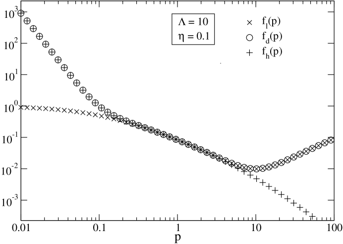
Figure 1: Components of the uniformly valid expansion of a simple function. Note that $f=f_{l}+f_{h}-f_{d}$. For small momenta one clearly sees $f_{h}$ and $f_{d}$ will cancel, for high momenta $f_{l}$ and $f_{d}$ will cancel, and in the middle one set will cancel, leaving $f$ uniformly approximated in all regions.

To complete our discussion of our simple function $f$, we discuss a problem that arises when integrating the uniformly valid approximation over the whole range $0<p<\infty$. We assume that the integral of the exact functions converges, so clearly if we use the entire uniformly valid expansion to approximate the function the integral will converge, producing an expansion in powers of $\eta/\Lambda$ of the exact integral. The problem arises only if this integration is performed term by term; in this case some of the terms can lead to divergent integrals. For one example, the two most divergent terms for large $p$ are:

$${p^{2}\over(p+\eta)\Lambda^{3}}-{p\over\Lambda^{3}}\ ,$$ (75)

each of which give rise to quadratically divergent integrals for $p$ near infinity. The first term also has subdominant linear and logarithmic divergences when it is expanded in powers of $\Lambda/p$. All these divergences are cancelled: the quadratic divergences cancel between these two terms, and the subdominant divergences are cancelled by other terms from $f_{d}$.

The divergences must cancel exactly, but it is convenient for analytic work to have a procedure that makes the integral of each term separately finite, without changing the integral of the sum of all terms. We can accomplish this goal by introducing a standardized subtraction to apply to each divergent integral to make it finite. For example, we could suggest the following set of standardized subtractions to make all integrals finite at their upper limit:

1. Positive powers of $p$ and constant terms independent of $p$ are dropped completely, e.g., $p^{n}$ is replaced by 0 for all $n\geq 0$.

2. A logarithmic divergent $1/p$ term, integrated to infinity, is subtracted out from $\Lambda$ to infinity.

According to these rules the $p/\Lambda^{3}$ term would be dropped completely, positive powers of $p$ for $p\gg\Lambda$ would be subtracted from the $p^{2}/\left((p+\eta)\Lambda^{2}\right)$ term, and the $1/p$ component of this term would be subtracted out only for $p>\Lambda$. To illustrate how this rule works, we exhibit the subtracted form for the integral over the first term:

$$\int^{\infty}_{0}dp\left\{{p^{2}\over(p+\eta)\Lambda^{2}}-{p\over\Lambda^{2}}+{\eta\over\Lambda^{2}}\right\}-\int^{\infty}_{\Lambda}{\eta^{2}\over p\Lambda^{2}}dp\ .$$ (76)

Note that a rule subtracting $1/p$ terms for all $p$ would not work, because they would introduce unwanted divergences for $p\to 0$. These rules do not change the overall integration of the uniformly valid approximation because all the subtractions cancel out.

A similar set of rules can be derived for handling divergences for $p\to 0$:

1. Negative powers of $p$ other than $1/p$ are dropped completely.

2. A logarithmically divergent $1/p$ term is subtracted out only for $0<p<\eta$. We use $\eta$ rather than $\Lambda$ because $1/p$ divergences for small $p$ typically emerge from functions involving $\eta$ rather than $\Lambda$, and this form for the subtraction ensures that such functions do not acquire an unwanted dependence on $\Lambda$ as well.

The application of this scheme is easy when given a simple function, but its real power is only seen when solving an integral equation in which the function is not known. Even though the function is not known, we can solve for the pieces of its uniformly valid expansion and this is our procedure for obtaining an expansion of $B_{3}$ and the wave function in powers of $B/\Lambda^{2}$.

In order to solve the complete set of equations, we also need an expansion for functions that depend on two momenta, $p$ and $q$, each of which range from $0$ to $\infty$. We do not present a full analysis of this expansion here, because it requires eleven regions. A full discussion is found in Mohr’s thesis Mohr03 .

VIII Leading Order Three-body Equation for Large $\Lambda$

We are now prepared to solve the three-body equations in the limit $\Lambda\rightarrow\infty$. To do this, we first need to find the leading-order approximation to the full integral equations using the method of uniformly valid expansions. We assume that all binding energies are much less than the cutoff and isolate approximations that are valid in various regions of momenta. It is conceptually straightforward to extend the calculation to systematically include higher-order corrections, but these will not affect the continuum limit that we isolate as a starting point. We will provide only those details that are required to qualitatively understand the results and once again refer the reader to Mohr’s thesis Mohr03 for details.

We start with a few definitions that will simplify notation somewhat:

$$\eta_{2} \equiv \sqrt{B_{2}},$$ (77)

$$\eta_{3} \equiv \sqrt{B_{3}}.$$ (78)

Using $\eta_{2}$ and $\eta_{3}$ in our equations allows us to deal with quantities that have the same dimension as the momentum variable. It also identifies their role in the expansion as the parameter $\eta$ from the previous chapter. In fact, we will occasionally use $\eta$ to generically refer to $\eta_{2}$ and $\eta_{3}$ in places where either is a valid alternative.

We use dimensionless couplings, $G_{2}\equiv\Lambda\,g_{2}$ and $G_{3}\equiv\Lambda^{4}\,g_{3}.$ Further, we note that $G_{3}$ enters the bound-state equation only as a multiplicative constant that is easier to work with:

$$\delta\equiv\frac{G_{3}\,\Phi_{1}}{\Lambda}.$$ (79)

$\delta$ will be found to remain finite for all values of the cutoff, and at the end of the calculation we can readily compute $\Phi_{1}$ to isolate $G_{3}$ and display the limit cycle. We will find that $\Phi_{1}$ is independent of $B_{3}$ to leading order, which is consistent with the fact that we have only one coupling $G_{3}$ with which we must renormalize the entire bound state spectrum.

Another dimensionless quantity, and perhaps the most important, is the replacement of the pseudo-wavefunction $\Phi(p)$ with

$$f(\eta_{2},\eta_{3},p,\Lambda)\equiv(p^{2}+\eta_{3}^{2}-\eta_{2}^{2})\Phi(p).$$ (80)

Like $\eta_{2}$ and $\eta_{3}$, its role in the expansion is easily seen to be the same as the function $f$ used in the previous chapter. Like $G_{2}$ and $G_{3}$, the dimensionless nature of $f$ will simplify future power counting. In addition, the $p^{2}$ term in the factor $p^{2}+\eta_{3}^{2}-\eta_{2}^{2}$ ensures that $f$ tends to be of ${\cal O}(1)$ throughout the entire range of $p$ while the $\eta_{3}^{2}-\eta_{2}^{2}$ term makes $f$ less prone to large numerical fluctuations than $\Phi$ when $B_{2}\simeq B_{3}$.

With these new definitions, the three-body bound-state equation (59) now takes the form

$$f(\eta_{2},\eta_{3},p,\Lambda) = \frac{p^{2}+\eta_{3}^{2}-\eta_{2}^{2}}{2\pi^{2}D\left(-\eta_{3}^{2}-\frac{3}{2}p^{2}\right)}\int_{0}^{\infty}dq\>\left[\frac{q^{2}}{q^{2}+\eta_{3}^{2}-\eta_{2}^{2}}\right.$$ (81)

$$\left.\times\int_{-1}^{1}dz\>\frac{U_{2}\left({\bf q}+\frac{1}{2}{\bf p}\right)U_{2}\left({\bf p}+\frac{1}{2}{\bf q}\right)}{\eta_{3}^{2}+2p^{2}+2q^{2}+2pqz}f(\eta_{2},\eta_{3},q,\Lambda)\right]$$

$$-~{}\delta\;\frac{(p^{2}+\eta_{3}^{2}-\eta_{2}^{2})D_{1}(p)}{G_{2}\Lambda^{2}D\left(-\eta_{3}^{2}-\frac{3}{2}p^{2}\right)}.$$

The process of expanding Eq. (81) is done in a series of steps. Because the $\delta$ term is simply added to the integral term, each can be expanded individually and then added together at the end. In addition, these terms are composed of other quantities like $D_{1}(p)$, $G_{2}$, etc. which have their own expansions in terms of $\eta/\Lambda$. The goal is to split the equation for $f$ into separate equations for $f_{l}$, $f_{d}$, and $f_{h}$, isolating and solving the leading order equations to produce a uniformly valid approximation for the wave function. The details of the calculation are not very enlightening, so we simply list the complete set of leading order equations that must be solved.

Pseudo-Wavefunctions:

We are able to precisely compute a cutoff integral over one variable of the three-body wave function. The fundamental equations for the calculation of these pseudo-wavefunctions are:

$$f_{l0}(\eta_{2},\eta_{3},p) = \frac{1}{4\pi^{2}D_{l0}(\eta_{2},\eta_{3},p)}\int_{0}^{\infty}dq\>\left[\frac{q\,(p^{2}+\eta_{3}^{2}-\eta_{2}^{2})}{p\,(q^{2}+\eta_{3}^{2}-\eta_{2}^{2})}\right.$$

$$\times\left.\ln\left(\frac{\eta_{3}^{2}+2p^{2}+2q^{2}+2pq}{\eta_{3}^{2}+2p^{2}+2q^{2}-2pq}\right)f_{l0}(\eta_{2},\eta_{3},q)\right],$$

$$\ f_{d0}(p) = \frac{p}{4\pi^{2}D_{d0}(p)}\int_{0}^{\infty}\frac{dq}{q}\,\ln\left(\frac{p^{2}+q^{2}+pq}{p^{2}+q^{2}-pq}\right)f_{d0}(q),$$

$$f_{h0}(p,\Lambda) = \frac{p^{2}}{2\pi^{2}D_{h0}(p,\Lambda)}\int_{0}^{\infty}dq\,\int_{-1}^{1}dz\,\frac{U_{2}\left({\bf q}+\frac{1}{2}{\bf p}\right)U_{2}\left({\bf p}+\frac{1}{2}{\bf q}\right)}{2p^{2}+2q^{2}+2pqz}f_{h0}(q,\Lambda),$$

$$\hskip 36.135pt-~{}\delta_{0}\,\frac{3h_{2}^{2}+8h_{2}+16}{128\sqrt{2}\,\pi^{3/2}}\left(\frac{D_{1h0}(p,\Lambda)}{D_{h0}(p,\Lambda)}\right)\left(\frac{p^{2}}{\Lambda^{2}}\right).$$

The intermediate range can be determined analytically Dan61 :

$$f_{d0}(p) = A\cos\left(s_{0}\ln\left(\frac{p}{\Lambda}\right)+\theta\right),$$

where we can choose $A=1$ because the bound state equations are homogeneous, $\theta$ is a phase determined by boundary conditions, and $s_{0}$ is the real, positive solution to the equation

$$\frac{8}{\sqrt{3}}\,\sinh\left(\frac{\pi s_{0}}{6}\right)=s_{0}\,\cosh\left(\frac{\pi s_{0}}{2}\right).$$ (86)

The value of $s_{0}$ to the precision we want is $1.006237825102$.

The $\Lambda$ dependence in Eq. (85) may be a bit misleading since Eq. (83) does not contain it. The cutoff is required because the argument of the logarithm is dimensionless. Making this choice is a matter of preference, and it could just as easily have been $\eta_{3}$. We discuss this renormalization prescription below; but first we need to show how choosing two binding energies uniquely determines one and only one bound state spectrum.

Clearly the choice of $B_{2}$ can be made independently of any modeling in the three-body system, so we take this and $B_{3}$ as input for Eq. (85). We assume that $B_{3}>B_{2}$ so that a stable three-body bound state exists. This determines $f_{l0}(p)$, which must map exactly on to $f_{d0}(p)$ for $p\gg\eta_{3}$. Once $\Lambda$ is chosen, $\theta$ in $f_{d0}$ is determined by the phase of $f_{l0}$, which is in turn determined by both $B_{2}$ and $B_{3}$. Finally, $f_{h0}(p)$ must map onto $f_{d0}(p)$ for $p\ll\Lambda$. The solution requires a phase and this fixes it. Given the phase in $f_{h0}(p)$, $\Phi_{1}$ is determined, which in turn yields $G_{3}$.

This explains how one three-body bound state is determined. The remaining allowed values of $B_{3}$ must produce the same phase $\theta$ as is produced by the value that is fixed to determine $\theta$. This produces both the remaining spectrum and the pseudo-wavefunction.

The remaining equations we require are:

$$D_{l0}(\eta_{2},\eta_{3},p) = \frac{\sqrt{\frac{3}{2}p^{2}+\eta_{3}^{2}}-\eta_{2}}{8\sqrt{2}\,\pi},$$ (87)

$$D_{d0}(p) = \frac{\sqrt{3}\,p}{16\pi},$$ (88)

$$D_{h0}(p,\Lambda) = \frac{p}{256\pi^{2}\Lambda^{4}}\left[\sqrt{3}\,\pi\left(4\Lambda^{2}-3h_{2}p^{2}\right)^{2}\left(1-\mathrm{Erf}\left(\frac{\sqrt{3}\,p}{\sqrt{2}\,\Lambda}\right)\right)\exp\left(\frac{3p^{2}}{2\Lambda^{2}}\right)\right.$$ (89)

$$+~{}3\sqrt{2\pi}\,h_{2}\Lambda p\left(\left(8+h_{2}\right)\Lambda^{2}-3h_{2}p^{2}\right)\Bigg{]},$$

$$D_{1l0}(\Lambda) = \frac{\Lambda\left(6\left(h_{3}^{2}+4h_{3}+12\right)+h_{2}\left(5h_{3}^{2}+12h_{3}+12\right)\right)}{576\sqrt{3}\,\pi^{3/2}},$$ (90)

$$D_{1d0}(\Lambda) = \frac{\Lambda\left(6\left(h_{3}^{2}+4h_{3}+12\right)+h_{2}\left(5h_{3}^{2}+12h_{3}+12\right)\right)}{576\sqrt{3}\,\pi^{3/2}},$$ (91)

$$D_{1h0}(p,\Lambda) = \frac{1}{4\pi^{2}}\int_{0}^{\infty}dq\>q^{2}\,\int_{-1}^{1}dz\>\frac{U_{2}({\bf q}+\frac{1}{2}{\bf p}\,)U_{3}(q)U_{3}(p)U_{3}({\bf p}+{\bf q}\,)}{2p^{2}+2q^{2}+2pqz},$$ (92)

$$G_{2} \equiv \Lambda g_{2},$$ (93)

$$G_{2,0} = \frac{128\sqrt{2}\,\pi^{3/2}}{3h_{2}^{2}+8h_{2}+16},$$ (94)

$$G_{3} \equiv \Lambda^{4}g_{3},$$ (95)

$$G_{3,0} = \frac{\delta_{0}}{G_{2,0}\,{\cal I}_{0}-D_{2,0}\,\delta_{0}/\Lambda^{4}},$$ (96)

$${\cal I}_{0} = \frac{3}{2\pi^{2}\Lambda^{2}}\int_{0}^{\infty}dp\,D_{1h0}(p,\Lambda)\,f_{h0}(p,\Lambda),$$ (97)

$$D_{2,0} = \frac{1}{8\pi^{4}}\int_{0}^{\infty}p^{2}dp\int_{0}^{\infty}q^{2}dq\int_{-1}^{1}dz\>\frac{U_{3}(q)^{2}U_{3}(p)^{2}U_{3}({\bf q}+{\bf p})^{2}}{2p^{2}+2q^{2}+2pqz}.$$ (98)

At this point we simply need to solve these equations numerically. We demonstrate that we achieve 10–12 digits of precision.

IX Discretization and Precision

Because a closed-form solution for either $f_{l0}$ or $f_{h0}$ is unknown, we must resort to numerical calculations of these functions as well as any energies or couplings. A common method for solving an integral equation involves changing the integration into a sum over discrete points. The integral equation then becomes a matrix equation easily solved by standard methods.

While this may appear straightforward, there are several practical issues to consider. For example, new limits on the integral equation must be determined. It is impossible to numerically integrate to infinity, so a suitable upper bound must be chosen. In our case, we use a logarithmic integration scale, which is critical in almost all problems amenable to renormalization, so a new lower bound to replace $0$ must also be determined. How the discrete points are chosen must be carefully considered. Fortunately, for our problem exponential convergence with the number of points can be achieved, as discussed below.

Each choice is a compromise between accuracy and size. For example, we could choose an upper limit that is extremely large (ensuring that we are “close” to infinity) and discrete points that are closely spaced (minimizing errors in the sum). The trade-off is that using more points requires using a larger matrix. Using $N$ discrete points will result in an $N\times N$ matrix with $N^{2}$ elements. If all numbers are double precision decimals, even 8000 points would be enough to overwhelm a computer with 512 MB of memory. This does not even take into account the time needed to process such a matrix. Obviously, the goal is to obtain the desired accuracy with a minimal number of points. We will discuss a few methods that drastically reduce the number of points we need.

In the following sections, we will assume that our goal is about 12 digits of accuracy. This high accuracy may not be necessary for most leading order calculations, but it is essential when studying leading corrections. Besides directly obtaining the equations for the $\Lambda\rightarrow\infty$ limit, one principal reason for expanding the three-body equation in powers of $\eta/\Lambda$ is to analyze the cutoff dependence. If we are attempting to study this behavior, we must be certain that our numerical errors are not larger than the corrections being studied; otherwise there is no way to distinguish the small corrections from the numerical “noise.”

IX.1 Transition to Mid-Momentum Function

One way to limit the size of the matrix is to limit the range over which the function must be integrated. We know that $f_{l0}$ and $f_{h0}$ approach $f_{d0}$ for $p\gg\eta$ and $p\ll\Lambda$ respectively. This allows us to replace either function with $\cos\left(s_{0}\ln(p/\Lambda)+\theta\right)$ in the appropriate range. The point at which we can make the switch is determined by the accuracy we desire. These limits are derived for the case of 12 digits of accuracy.

For $p\gg\eta$, the equation for $f_{l0}$ can be written as

$$f_{l0}(\eta_{2},\eta_{3},p)=\frac{4(1+\eta_{3}^{2}/p^{2}-\eta_{2}^{2}/p^{2})}{\sqrt{3}\pi\left(\sqrt{1+(2\eta_{3}^{2})/(3p^{2})}-(\sqrt{2}\eta_{2})/(\sqrt{3}p)\right)}\int_{0}^{\infty}dq\>\frac{q}{q^{2}+\eta_{3}^{2}-\eta_{2}^{2}}$$

$$\times\left[\ln\left(\frac{p^{2}+q^{2}+pq}{p^{2}+q^{2}-pq}\right)+\frac{\eta_{3}^{2}}{2p^{2}+2q^{2}+2pq}-\frac{\eta_{3}^{2}}{2p^{2}+2q^{2}-2pq}\right]f_{l0}(\eta_{2},\eta_{3},q).$$ (99)

Here we have treated $\eta/p$ as a small quantity and perturbatively expanded all factors. As long as both $\eta_{2}/p$ and $\eta_{3}/p$ are less than $10^{-12}$, this equation will match the one for $f_{d0}$ to 12 digits. Of course, $\eta_{3}$ must be greater than $\eta_{2}$ since we are considering only stable bound states. This means that $p\simeq 10^{12}\,\eta_{3}$ sets the limit above which $f_{l0}$ can be replaced by $f_{d0}$. In practice, we must have enough data points above this limit to ensure that our cosine fit is accurate to 12 digits also. Therefore, we will use an actual limit of $p=10^{15}\,\eta_{3}$.

Similarly, we can expand the equation for $f_{h0}$ in the region $p\ll\Lambda$. Notice that in this region $D_{1h0}(p,\Lambda)$ approaches $D_{1d0}(\Lambda)$ which is proportional to $\Lambda$, and the function $D_{h0}(p,\Lambda)$ becomes equal to $D_{d0}(p)=\sqrt{3}\,p/16\pi$. In the $f_{h0}$ integral equation, the momentum-dependent part of the three-body interaction becomes

$$\left(\frac{p^{2}}{\Lambda^{2}}\right)\left(\frac{D_{1h0}(p,\Lambda)}{D_{h0}(p,\Lambda)}\right)\stackrel{{\scriptstyle p\ll\Lambda}}{{\longrightarrow}}\left(\frac{p^{2}}{\Lambda^{2}}\right)\left(\frac{D_{1d0}(\Lambda)}{D_{d0}(p)}\right)\propto\frac{p}{\Lambda}.$$ (100)

Since the leading order mid-momentum equation has no three-body interaction term, the above term will equal zero to 12 digits if we choose $p\sim 10^{-12}\,\Lambda$.

The integral part for $f_{h0}$ looks like

$$\frac{p^{2}}{2\pi^{2}D_{h0}(p,\Lambda)}\int_{0}^{\infty}dq\,\int_{-1}^{1}dz\,\frac{U_{2}\left({\bf q}+\frac{1}{2}{\bf p}\right)U_{2}\left({\bf p}+\frac{1}{2}{\bf q}\right)}{2p^{2}+2q^{2}+2pqz}f_{h0}(q,\Lambda).$$ (101)

We have already stated that $D_{h0}(p,\Lambda)$ approaches $D_{d0}(p)$, but more importantly, it approaches like

$$D_{h0}(p,\Lambda)\stackrel{{\scriptstyle p\ll\Lambda}}{{\longrightarrow}}D_{d0}(p)\left[1+\left(\frac{\sqrt{3}\,(h_{2}^{2}+8h_{2}-16)}{8\sqrt{2\pi}}\right)\frac{p}{\Lambda}\right].$$ (102)

It will therefore equal $D_{d0}$ to 12 digits if $p\sim 10^{-12}\,\Lambda$. This limit also applies to the integrand itself, so we may replace $f_{h0}$ with $f_{d0}$ for values of $p$ less than ${\cal O}(10^{-12}\,\Lambda)$. In practice however, we use a limit of $p=10^{-17}\,\Lambda$ to ensure that we have enough points below this region to fit the cosine behavior.

IX.2 New Integration Limits

For the case of $f_{h0}$, we have limited the range of integration to be $10^{-17}\,\Lambda$ to $\infty$. (Below this range, we use $f_{d0}$.) Naturally, we cannot integrate to infinity and instead must find a new limit to replace it. Let us call this limit $\lambda$. We choose $\lambda$ such that

$$\frac{p^{2}}{2\pi^{2}D_{h0}(p,\Lambda)}\int_{\lambda}^{\infty}dq\,\int_{-1}^{1}dz\,\frac{U_{2}\left({\bf q}+\frac{1}{2}{\bf p}\right)U_{2}\left({\bf p}+\frac{1}{2}{\bf q}\right)}{2p^{2}+2q^{2}+2pqz}f_{h0}(q,\Lambda)<{\cal O}(10^{-12}).$$ (103)

The exponentials in $U_{2}$ suggest that the integrand should die off quickly, allowing us to make an initial guess for $\lambda$ using

$$\mathrm{e}^{-\lambda^{2}/\Lambda^{2}}=10^{-12}.$$ (104)

This gives an initial value of $\lambda\simeq 5.25\,\Lambda$. However, the double integral makes the analysis harder since we cannot determine the exact behavior. We must resort to numerical computation, and some sample calculations reveal that a limit of $\lambda=10\,\Lambda$ is sufficient for our purposes.

From $10^{-17}\,\Lambda$ down to 0, $f_{h0}$ is replaced by $f_{d0}$. We would like to replace the $0$ limit with a larger value that still maintains our desired accuracy. Even though we know the analytic solution for $f_{d0}$, narrowing the range of integration will reduce our computational effort. Call this new lower limit $\epsilon$, which is chosen so that

$$\frac{p^{2}}{2\pi^{2}D_{h0}(p,\Lambda)}\int_{0}^{\epsilon}dq\,\int_{-1}^{1}dz\,\frac{U_{2}\left({\bf q}+\frac{1}{2}{\bf p}\right)U_{2}\left({\bf p}+\frac{1}{2}{\bf q}\right)}{2p^{2}+2q^{2}+2pqz}f_{d0}(q,\Lambda)<{\cal O}(10^{-12}).$$ (105)

We assume that $\epsilon\ll 10^{-17}\,\Lambda<p$. To within 12 digits of accuracy, the $z$ integration can be written as

$$\int_{-1}^{1}dz\,\frac{U_{2}\left({\bf q}+\frac{1}{2}{\bf p}\right)U_{2}\left({\bf p}+\frac{1}{2}{\bf q}\right)}{2p^{2}+2q^{2}+2pqz} = \int_{-1}^{1}dz\,\frac{U_{2}\left({\bf p}/2\right)U_{2}\left({\bf p}\right)}{2p^{2}+2pqz}$$ (106)

$$= \frac{1}{2pq}\,U_{2}\left({\bf p}/2\right)U_{2}\left({\bf p}\right)\,\ln\left(\frac{p^{2}+pq}{p^{2}-pq}\right).$$

Since $q\ll p$, the logarithm can be approximated as $2q/p$. Our constraint for $\epsilon$ now becomes

$$\frac{1}{2\pi^{2}D_{h0}(p,\Lambda)}\,U_{2}\left({\bf p}/2\right)U_{2}\left({\bf p}\right)\,\int_{0}^{\epsilon}dq\,f_{d0}(q)<{\cal O}(10^{-12}).$$ (107)

The values of $p$ are of the same order as $\Lambda$, so we expect the value of $U_{2}$ to be ${\cal O}(1)$. The function $f_{d0}$ is also ${\cal O}(1)$, so it is simply replaced by $1$ in this approximation. This leaves an integral with a value of $\epsilon$. When combined with $D_{h0}(p,\Lambda)\sim{\cal O}(p)$, we find that $\epsilon/p<{\cal O}(10^{-12})$. The smallest value for $p$ is $10^{-17}\,\Lambda$, implying that $\epsilon\simeq 10^{-29}\,\Lambda$. In practice, this value is sufficient for 12 digits of accuracy.

Having replaced the limits for $f_{h0}$, we move on to $f_{l0}$. Again, we must find a finite upper limit to substitute for infinity. For $p>10^{15}\,\eta_{3}$, $f_{l0}$ is replaced by $f_{d0}$. This new limit, $\lambda$, is determined by the condition

$$\frac{(p^{2}+\eta_{3}^{2}-\eta_{2}^{2})}{4\pi^{2}p\,D_{l0}(\eta_{2},\eta_{3},p)}\int_{\lambda}^{\infty}dq\>\left[\frac{1}{q}\ln\left(\frac{p^{2}+q^{2}+pq}{p^{2}+q^{2}-pq}\right)f_{d0}(q)\right]$$

$$\simeq\frac{(p^{2}+\eta_{3}^{2}-\eta_{2}^{2})}{4\pi^{2}p\,D_{l0}(\eta_{2},\eta_{3},p)}\int_{\lambda}^{\infty}\frac{dq}{q}\>\left(\frac{2p}{q}\right)f_{d0}(q)$$

$$=\frac{(p^{2}+\eta_{3}^{2}-\eta_{2}^{2})}{2\pi^{2}\,D_{l0}(\eta_{2},\eta_{3},p)}\int_{\lambda}^{\infty}\frac{dq}{q^{2}}\>f_{d0}(q)$$

$$\sim\frac{(p^{2}+\eta_{3}^{2}-\eta_{2}^{2})}{2\pi^{2}\,D_{l0}(\eta_{2},\eta_{3},p)}\int_{\lambda}^{\infty}\frac{dq}{q^{2}}$$

$$=\frac{(p^{2}+\eta_{3}^{2}-\eta_{2}^{2})}{2\pi^{2}\,D_{l0}(\eta_{2},\eta_{3},p)}\,\left(\frac{1}{\lambda}\right)\leq{\cal O}(10^{-12}),$$ (108)

where we have used the fact that $q\gg p\sim\eta_{3}$. For values of $p$ much larger than $\eta_{3}$, the term in Eq. (108) is proportional to $p/\lambda$. The largest value $p$ can obtain is $10^{15}\,\eta_{3}$, implying $\lambda=10^{27}\,\eta_{3}$. Numerical calculations verify that this limit is sufficient to assure the desired accuracy.

Finally, we must replace the lower limit for $f_{l0}$ with a non-zero value $\epsilon$ that we assume to be much smaller than $\eta_{3}$. Our requirement is that

$$\frac{(p^{2}+\eta_{3}^{2}-\eta_{2}^{2})}{4\pi^{2}p(\eta_{3}^{2}-\eta_{2}^{2})D_{l0}(\eta_{2},\eta_{3},p)}\int_{0}^{\epsilon}dq\,q\ln\left(\frac{\eta_{3}^{2}+2p^{2}+2pq}{\eta_{3}^{2}+2p^{2}-2pq}\right)f_{l0}(\eta_{2},\eta_{3},q)<{\cal O}(10^{-12}).$$ (109)

Expanding the logarithm to ${\cal O}(q)$ yields

$$\frac{(p^{2}+\eta_{3}^{2}-\eta_{2}^{2})}{\pi^{2}(\eta_{3}^{2}-\eta_{2}^{2})(\eta_{3}^{2}+2p^{2})D_{l0}(\eta_{2},\eta_{3},p)}\int_{0}^{\epsilon}dq\,q^{2}\,f_{l0}(\eta_{2},\eta_{3},q)<{\cal O}(10^{-12}).$$ (110)

For small values of $q$, we will find that $f_{l0}$ is approximately constant and of ${\cal O}(1)$. Therefore, the integral is roughly equal to $\epsilon^{3}$. If $p\ll\eta_{3}$ or $p\sim\eta_{3}$, then Eq. (110) is ${\cal O}(\epsilon^{3}/\eta^{3})$. If $p\gg\eta_{3}$, then it is ${\cal O}(\epsilon^{3}/p\eta_{3}^{3})<{\cal O}(\epsilon^{3}/\eta^{3})$. This seems to imply that a value of $\epsilon\simeq 10^{-4}\,\eta_{3}$ is adequate.

Unfortunately, using this value of $\epsilon$ will result in poor accuracy when $\eta_{2}\simeq\eta_{3}$. This is a result of the $(\eta_{3}^{2}-\eta_{2}^{2})$ term in the denominator of Eq. (110). Originally, this was our approximation to the term $(q^{2}+\eta_{3}^{2}-\eta_{2}^{2})$ in the integral equation. When the energies are nearly equal, our approximation needs to be $q^{2}$. The condition on $\epsilon$ should now become

$$\frac{(p^{2}+\eta_{3}^{2}-\eta_{2}^{2})}{\pi^{2}(\eta_{3}^{2}+2p^{2})D_{l0}(\eta_{2},\eta_{3},p)}\int_{0}^{\epsilon}dq\,f_{l0}(\eta_{2},\eta_{3},q)<{\cal O}(10^{-12}).$$ (111)

The integral is roughly equal to $\epsilon$, and the entire term is ${\cal O}(\epsilon/\eta)$. This means we must use the lower limit $\epsilon=10^{-12}\,\eta_{3}$.

These derivations are general enough to determine the appropriate limits for other cases of desired accuracy. Keep in mind however that the limits must always be tested numerically to ensure that they are indeed sufficient.

IX.3 Discrete Point Spacing

Now that we have limits in place, we must choose the discrete values of $q$ within these limits at which to evaluate our functions. We employ discrete points that are equally spaced on a logarithmic scale. There are two main reasons for making this choice.

First, we have already seen that $f_{d0}=\cos\left(s_{0}\ln(p/\Lambda)+\theta\right)$ is periodic on a logarithmic scale. In fact, other functions have similar behavior, including $G_{3}$. It makes sense that a logarithmic spacing is suited to capturing the behavior of the system.

Second, and far more important, by choosing points in this manner an integration of $q$ from $0$ to $\infty$ becomes an integration of $\ln(q)$ from $-\infty$ to $\infty$. By equally spacing points on this log scale, we can achieve convergence that improves exponentially with the spacing Tadmor , as opposed to the more typical power law convergence. This drastically reduces the number of points needed to achieve our desired accuracy. For instance, to cover the range of $f_{l0}$ from $10^{-12}\,\eta_{3}$ to $10^{15}\,\eta_{3}$, and maintain 12 digits of accuracy, we can space our points by $p_{n+1}=p_{n}\mathrm{e}^{0.2}$. This requires only about 300 points. Exponential convergence with the number of point is extremely powerful and it is not widely appreciated that this is ever possible. A simple demonstration (with minor errors) can be found in an appendix in Mohr’s thesis Mohr03 . Figure 2 illustrates this exponential convergence which eventually terminates due to roundoff errors.

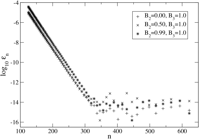
Figure 2: Relative error in the phase appearing in pseudo-wave functions as a function of the number of points used in the discretized approximation for several pairs of two-body and three-body binding energies.

X Discretized Equations

The discretized integral equations are shown below. Here, $\Delta$ represents the momentum spacing, and the momentum values are related by the equation $p_{n+1}=p_{n}\,\mathrm{e}^{\Delta}$. The identity matrix is represented by $I_{nm}$, and the ceiling function represented by $\lceil x\rceil$ returns an integer value $n$ such that $(n-1)<x\leq n$.

Low-Momentum: These are easily derived from Eq. (83). The value of $n$ for $p_{n}$ ranges from 0 to $N_{mid}$, while the value of $m$ for $q_{m}$ ranges from 0 to $N_{max}$. These are defined as: $p_{0}=10^{-12}\,\eta_{3}$, $N_{mid}=\lceil\ln(10^{27})/\Delta\rceil$, and $N_{max}=\lceil\ln(10^{39})/\Delta\rceil$ .

$$\sum_{m=0}^{N_{mid}}\left(M_{nm}-I_{nm}\right)\,f_{l0}(p_{m})=b_{n},$$ (112)

$$M_{nm}=\frac{\Delta}{4\pi^{2}D_{l0}(\eta_{2},\eta_{3},p_{n})}\frac{q_{m}^{2}(p_{n}^{2}+\eta_{3}^{2}-\eta_{2}^{2})}{p_{n}(q_{m}^{2}+\eta_{3}^{2}-\eta_{2}^{2})}\ln\left(\frac{\eta_{3}^{2}+2p_{n}^{2}+2q_{m}^{2}+2p_{n}q_{m}}{\eta_{3}^{2}+2p_{n}^{2}+2q_{m}^{2}-2p_{n}q_{m}}\right),$$ (113)

$$b_{n}=-\frac{\Delta(p_{n}^{2}+\eta_{3}^{2}-\eta_{2}^{2})}{4\pi^{2}p_{n}D_{l0}(\eta_{2},\eta_{3},p_{n})}\sum_{m=N_{mid}+1}^{N_{max}}\left[\ln\left(\frac{\eta_{3}^{2}+2p_{n}^{2}+2q_{m}^{2}+2p_{n}q_{m}}{\eta_{3}^{2}+2p_{n}^{2}+2q_{m}^{2}-2p_{n}q_{m}}\right)\right.$$

$$\hskip 144.54pt\left.\times\cos\left(s_{0}\ln\left(\frac{q_{m}}{\Lambda}\right)+\theta\right)\right].$$ (114)

High-Momentum: The value of $n$ for $p_{n}$ ranges from 0 to $N_{max}$, while the value of $m$ for $q_{m}$ ranges from $-N_{min}$ to $N_{max}$. These are defined as: $p_{0}=10^{-17}\,\Lambda$, $N_{max}=\lceil\ln(10^{18})/\Delta\rceil$, and $N_{min}=\lceil\ln(10^{12})/\Delta\rceil$ .

$$\sum_{m=0}^{N_{max}}\left(M_{nm}-I_{nm}\right)\,f_{h0}(p_{m})=a_{n}+\delta_{0}\,b_{n},$$ (115)

$$M_{nm}=\frac{q_{m}p_{n}^{2}\Delta}{2\pi^{2}D_{h0}(p_{n},\Lambda)}K(p_{n},q_{m}),$$ (116)

$$a_{n}=-\frac{p_{n}^{2}\Delta}{2\pi^{2}D_{h0}(p_{n},\Lambda)}\sum_{m=-N_{min}}^{-1}q_{m}\,K(p_{n},q_{m})\cos\left(s_{0}\ln\left(\frac{q_{m}}{\Lambda}\right)+\theta\right),$$ (117)

$$b_{n}=\frac{p_{n}^{2}D_{1h0}(p_{n},\Lambda)}{\Lambda^{2}G_{2,0}D_{h0}(p_{n},\Lambda)},$$ (118)

$$K(p_{n},q_{m}) = \frac{\Delta}{2\Lambda^{2}}\sum_{k=-200}^{200}\left[(1-z_{k}^{2})\left(1+h_{2}\left(\frac{q_{m}^{2}}{\Lambda^{2}}+\frac{q_{m}p_{n}z_{k}}{\Lambda^{2}}+\frac{p_{n}^{2}}{4\Lambda^{2}}\right)\right)\right.$$ (119)

$$\times\left(1+h_{2}\left(\frac{p_{n}^{2}}{\Lambda^{2}}+\frac{q_{m}p_{n}z_{k}}{\Lambda^{2}}+\frac{q_{m}^{2}}{4\Lambda^{2}}\right)\right),$$

$$\left.\times\frac{\exp\left(-(5p_{n}^{2}+8p_{n}q_{m}z_{k}+5q_{m}^{2})/(4\Lambda^{2})\right)}{2\left(p_{n}^{2}/\Lambda^{2}+q_{m}^{2}/\Lambda^{2}+p_{n}q_{m}z_{k}/\Lambda^{2}\right)}\right],$$

$$z_{k}=\frac{\mathrm{e}^{0.2\,k}-1}{\mathrm{e}^{0.2\,k}+1}.$$ (120)

The hyperbolic tangent discretization we use for the angular integral, with 401 angular points, has been numerically verified to exceed our needs over the entire range of binding energies we explore. There may be equally good or better choices.

XI Analytic and Numerical Results

A computer program to solve the discretized integral equations can be implemented with the help of some basic numerical algorithms. Once completed, it can be used to generate highly accurate results and analyze the three-body system. Nonetheless, attempts to extract analytic results should not be overlooked. Even some of the most general properties of the integral equations allow us to draw conclusions about the behavior of the system.

We begin this chapter with analytic results obtained from studying the leading order integral equations. These results include statements about the cutoff dependence of bound-state energies and the phase for $f_{d0}$. A proof for the cyclic behavior of $\delta_{0}$ is given, which is then used to infer similar behavior for $G_{3}$.

Following the analytic results is a section containing numerical solutions to the integral equations. Here we examine behavior that cannot be determined analytically. Solutions for the functions $f_{l0}$ and $f_{h0}$ are shown, and the cutoff dependence of $G_{3}$ is calculated. Some relations that are proven analytically are also verified numerically.

In Section VIII, we saw that Eq. (VIII) contains no $\Lambda$ dependence, making the function $f_{l0}(p)$ cutoff-independent. However, for values of $p\gg\eta_{3}$, the solution must behave like $f_{d0}(p)=\cos\left(s_{0}\,\ln\left(p/\Lambda\right)+\theta\right)$, which explicitly has the cutoff in it. The only way these two equations can be reconciled is if $\theta$ contains cutoff dependence of the form $s_{0}\,\ln(\Lambda)$. Any remaining part of $\theta$ must be a function of $\eta_{2}$ and $\eta_{3}$. Therefore, we can write

$$\theta=s_{0}\,\ln\left(\Lambda/\eta_{3}\right)+\tilde{\theta}\left(\eta_{2}/\eta_{3}\right),$$ (121)

where $\tilde{\theta}$ is a dimensionless function of the ratio $\eta_{2}/\eta_{3}$. This relation holds for any values of $\eta_{2}$ and $\eta_{3}$, including all $\eta_{3}$ values corresponding to multiple bound states with the same $\eta_{2}$. Using $\eta_{3}$ in the ratio with $\Lambda$ is a matter of choice. Any quantity composed of $\eta_{2}$ and $\eta_{3}$ with the same dimension as $\Lambda$ would work just as well; however, we need to allow $\eta_{2}=0$, so $\eta_{2}$ alone is a poor choice.

While Eq. (121) is quite simple, it has many interesting consequences. As we mentioned earlier, two different three-body bound states in the same spectrum must have the same phase $\theta$. Suppose that we choose some fixed values for $\eta_{2}$ and $\eta_{3}$ and make them cutoff-independent by choosing the appropriate $\Lambda$ dependence for $G_{2}$ and $G_{3}$. This might be desirable if we are trying to match those energies to experimental data. The phase for the solution in this case is

$$\theta_{\Lambda}=s_{0}\,\ln\left(\Lambda/\eta_{3}\right)+\tilde{\theta}\left(\eta_{2}/\eta_{3}\right),$$ (122)

for some given cutoff $\Lambda$. If the cutoff is changed, $G_{2}$, $G_{3}$, and $\theta_{\Lambda}$ will all change with it, but $\eta_{2}$, $\eta_{3}$, and $\tilde{\theta}(\eta_{2}/\eta_{3})$ will not.

Imagine now that we find a second three-body bound-state solution with the same phase. Let us call its energy $\bar{\eta}_{3}$. The phase for this solution is

$$\bar{\theta}_{\Lambda}=s_{0}\,\ln\left(\Lambda/\bar{\eta}_{3}\right)+\tilde{\theta}\left(\eta_{2}/\bar{\eta}_{3}\right),$$ (123)

which must be equal to $\theta_{\Lambda}$ by assumption. This results in the relation

$$s_{0}\,\ln\left(\bar{\eta}_{3}/\eta_{3}\right)=\tilde{\theta}\left(\eta_{2}/\bar{\eta}_{3}\right)-\tilde{\theta}\left(\eta_{2}/\eta_{3}\right).$$ (124)

If the cutoff is now changed to a new value $\Lambda^{\prime}$, the original data gives a phase of

$$\theta_{\Lambda^{\prime}}=s_{0}\,\ln\left(\Lambda^{\prime}/\eta_{3}\right)+\tilde{\theta}\left(\eta_{2}/\eta_{3}\right).$$ (125)

The question is whether $\bar{\eta}_{3}$ is still a valid solution. Its new phase is

$$\bar{\theta}_{\Lambda^{\prime}} = s_{0}\,\ln\left(\Lambda^{\prime}/\bar{\eta}_{3}\right)+\tilde{\theta}\left(\eta_{2}/\bar{\eta}_{3}\right)$$ (126)

$$= s_{0}\,\ln\left(\Lambda^{\prime}/\bar{\eta}_{3}\right)+\left[s_{0}\,\ln\left(\bar{\eta}_{3}/\eta_{3}\right)+\tilde{\theta}\left(\eta_{2}/\eta_{3}\right)\right]$$

$$= s_{0}\,\ln\left(\Lambda^{\prime}/\eta_{3}\right)+\tilde{\theta}\left(\eta_{2}/\eta_{3}\right)$$

$$= \theta_{\Lambda^{\prime}}.$$

Since the phases still match, $\bar{\eta}_{3}$ is still a bound-state solution. This remains true for any cutoff, implying that $\bar{\eta}_{3}$ is also cutoff-independent like $\eta_{3}$. Of course, the same statement applies to any other three-body bound state making the entire spectrum completely independent of $\Lambda$. Such behavior should come as no surprise since the leading order equations represent the $\Lambda\rightarrow\infty$ limit. Keep in mind that this is true for any other physical quantity, but does not apply to the couplings. Obviously, it is the cutoff dependence of the couplings that enables the bound states to be cutoff independent. We have shown that a single three-body contact interaction allows us to renormalize the entire three-body bound-state spectrum.

Just as $f_{l0}$ has no dependence on $\Lambda$, neither does it have any dependence on $h_{2}$. As a consequence, $h_{2}$ has no effect at leading order on the binding energies or other physical quantities. It does appear in the equation for $f_{l1}$ however, showing that it is needed when considering first order corrections. Because we work only to leading order, we use $h_{2}=0$ below unless stated otherwise.

We now turn to the equation for $f_{h0}(p)$:

$$f_{h0}(p,\Lambda)=\frac{p^{2}}{2\pi^{2}D_{h0}(p,\Lambda)}\int_{0}^{\infty}dq\,\int_{-1}^{1}dz\,\frac{U_{2}\left({\bf q}+\frac{1}{2}{\bf p}\right)U_{2}\left({\bf p}+\frac{1}{2}{\bf q}\right)}{2p^{2}+2q^{2}+2pqz}f_{h0}(q,\Lambda)$$

$$\hskip 36.135pt-~{}\delta_{0}\,\frac{3h_{2}^{2}+8h_{2}+16}{128\sqrt{2}\,\pi^{3/2}}\left(\frac{D_{1h0}(p,\Lambda)}{D_{h0}(p,\Lambda)}\right)\left(\frac{p^{2}}{\Lambda^{2}}\right).$$ (127)

The dependence on $p$ and $\Lambda$ has been explicitly shown. Since $f_{h0}$ is dimensionless, only the ratio $p/\Lambda$ can occur in the function. Furthermore, there is a dependence upon $h_{2}$ and $\theta$. The $h_{2}$ dependence comes from its appearance in the function $U_{2}(p)$, either directly in the integral or indirectly in $D_{h0}$ and $D_{1h0}$. The $\theta$ dependence is a result of $f_{h0}$ approaching $f_{d0}$ for $p\ll\Lambda$.

Assuming that $\Lambda$ is held fixed, choosing a value for $\delta_{0}$ will uniquely determine the phase. Thus, we can view the phase as a function of the coupling, $\theta(\delta_{0})$. Conversely, choosing a phase determines the coupling, so it is equally valid to treat the coupling as a function of the phase, $\delta_{0}(\theta)$. The coupling $\delta_{0}$ can also have a dependence upon $h_{2}$ but not upon $\Lambda$. The reason is that $\delta_{0}$ is dimensionless and there is no other quantity available to form a dimensionless ratio with $\Lambda$.

With this in mind, consider a solution to Eq. (127) with a coupling of $\delta_{0}(\theta)$ and a function $f_{h0}(p)$ that behaves asymptotically as $\cos\left(s_{0}\,\ln\left(p/\Lambda\right)+\theta\right)$ for small $p$. For a phase of $\theta+2\pi$, the cosine behavior will remain unchanged. We may therefore conclude that

$$\delta_{0}(\theta+2\pi)=\delta_{0}(\theta),$$ (128)

showing that the coupling exhibits periodic behavior. If we apply the operator $-\partial^{2}/\partial\theta^{2}$ to both sides of (127), we find once again that the asymptotic cosine behavior is the same. This implies

$$-\frac{\partial^{2}\delta_{0}}{\partial\theta^{2}}=\delta_{0}(\theta).$$ (129)

The conclusion to be drawn is that the coupling may be written as a cosine function with some amplitude ${\cal A}$ and phase $\phi$. These two parameters will contain any $h_{2}$ dependence that $\theta$ may possess, so we shall write

$$\delta_{0}(\theta)={\cal A}(h_{2})\,\cos\left(\theta+\phi(h_{2})\right).$$ (130)

The equation relating $\delta_{0}$ and $G_{3}$,

$$G_{3,0}=\frac{\delta_{0}}{G_{2,0}\,{\cal I}_{0}-D_{2,0}\,\delta_{0}/\Lambda^{4}},$$ (131)

shows that whenever $\delta_{0}$ is zero, so is $G_{3}$. Since two adjacent zeros of $\delta_{0}$ occur when the cutoffs satisfy

$$\theta_{\Lambda^{\prime}}-\theta_{\Lambda}=s_{0}\,\ln\left(\frac{\Lambda^{\prime}}{\Lambda}\right)=\pi,$$ (132)

the adjacent zeros of $G_{3}(\Lambda)$ should be spaced by a cutoff factor of $\Lambda^{\prime}/\Lambda=\exp(\pi/s_{0})\simeq 22.69438259536$. This suggests that $G_{3}(\Lambda)$ may also possess cyclic behavior, but this must be verified numerically, which is done below.

We begin our numerical investigation by considering solutions for the functions $f_{l0}$ and $f_{h0}$ which lead to an approximation for the complete function $f(p)$. Next, the cutoff independence of the three-body spectrum is verified, followed by an analysis of the coupling constants. These numerical results are confirmed by Wilson’s calculations Wil00 .

XI.1 Pseudo-Wave Functions

Figure 3 shows the numerical solution for $f_{l0}(p)$ in the case of $B_{2}=0.1$, $B_{3}=1.0$, and $\Lambda=10^{8}$. Notice that it is constant for small values of momentum and then takes on the cosine behavior of $f_{d0}$ as $p$ becomes large. Since the behavior of the solution to the low-momentum equation is determined by the ratio $B_{2}/B_{3}$, this figure is representative of all solutions, as demonstrated explicitly in Mohr’s thesis Mohr03 .

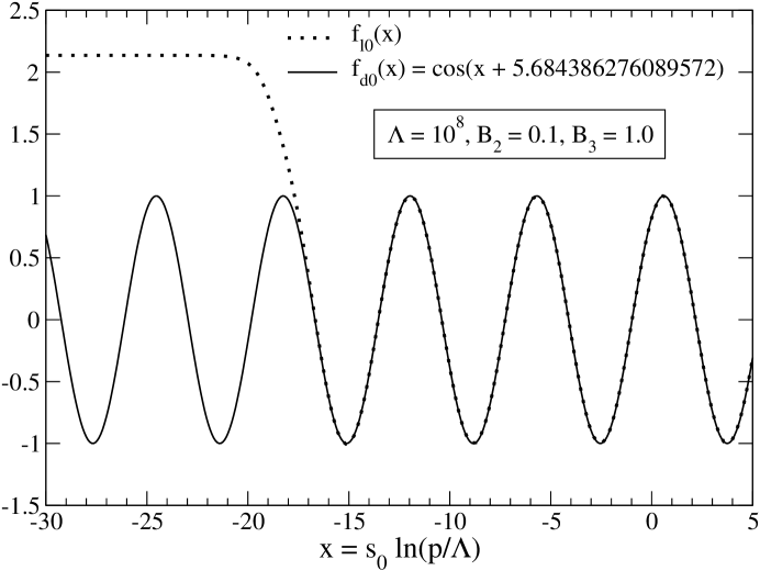
Figure 3: Numerical solution of $f_{l0}(p)$ shown matching on to $f_{d0}(p)$ for the case of $B_{2}=0.1$, $B_{3}=1.0$, and $\Lambda=10^{8}$.

This binding energy leads to $\theta=5.684386276089572...$, and with $\Lambda=10^{8}$ we find the numerical solution for the function $f_{h0}(p)$ shown in Figure 5. This is the high-momentum function corresponding to the low-momentum function in Figure 3. For all $f_{h0}$ solutions, we see the cosine behavior for $p\ll\Lambda$ and a suppression of large momentum values when $p>\Lambda$. This suppression is an effect of the Gaussian behavior of $U_{2}$.

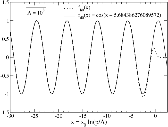
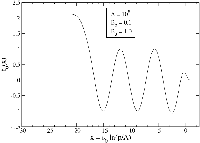
Figure 4: Numerical solution of $f_{h0}(p)$ for the case $\theta=5.684386276089572$ and $\Lambda=10^{8}$. The dashed line is the best-fit cosine curve that matches the low-momentum behavior.

Figure 5: Numerical solution of $f_{0}(p)$ for the case of $B_{2}=0.1$, $B_{3}=1.0$, and $\Lambda=10^{8}$.

Combining $f_{l0}$, $f_{d0}$ and $f_{h0}$, we see the overall leading order behavior for the function $f(p)$. Figure 5 shows $f_{l0}+f_{h0}-f_{d0}$ for $B_{2}=0.1$, $B_{3}=1.0$, and $\Lambda=10^{8}$. All solutions show this same qualitative behavior, with a flat plateau at low momenta going to cosine behavior for medium momenta and finally decaying rapidly at large momenta above the cutoff. Increasing the cutoff while changing the coupling so that the phase remains constant simply extends the cosine region, pushing the eventual decay to higher momenta.

Several bound states typically exist for the same values of $B_{2}$ and $\Lambda$. In the case of $B_{2}=1.0$ and $B_{3}=1.0$ for $\Lambda=10^{8}$, there exist states of energy $B_{3}=6.7502901502599$ and $B_{3}=1406.130393204$. The solutions of $f_{l0}$ for these energies are shown in Figure 6. All of the functions are very similar. The only real difference is in the length of the initial plateau. As the bound-state energies become larger, the flat region becomes longer, joining the cosine near later peaks. For a fixed cutoff there are a finite number of solutions because the cosine terminates near the cutoff, but as the cutoff is extended and further periods of the cosine result, additional bound states appear.

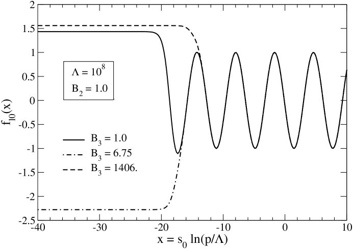
Figure 6: Numerical solution of $f_{l0}(p)$ for three bound states using $B_{2}=1.0$ and $\Lambda=10^{8}$. The three-body bound state energies are 1.0, 6.7502901502599 and 1406.1303932044.

XI.2 Three-Body Binding Energies

Above we proved that the three-body bound-state spectrum is cutoff independent to leading order. We choose $B_{2}=0$ (for which there is a limit cycle that persists to arbitrarily small cutoffs) and let $G_{3}$ change with $\Lambda$ so that the state $B_{3}=1.0$ is held constant. For this special case there are an infinite number of low-lying bound states as shown by Efimov Efi70 ; Efi71 . Two other states, one shallower and one deeper, are calculated as the cutoff changes. Since very small fluctuations are impossible to see in a plot, Table 1 shows the calculated energies for several values of $\Lambda$. Using Efimov’s result that the ratio of adjacent binding energies is $\exp(2\pi/s_{0})$ when $B_{2}=0$ Efi70 ; Efi71 , the relative error for each calculation can be determined and is also given in the table. This illustrates that each energy is cutoff-independent to about 12 digits and also matches the true value to the same accuracy. As an additional example, Table 2 shows the case of $B_{2}=B_{3}=1.0$ and considers the next two deeper states as $\Lambda$ changes. The binding energies are approximately 6.75029 and 1406.13. These energies have been previously calculated by Bedaque et al. BHK99b and by Braaten, Hammer and Kusunoki BHK03 using a method that gives at most two digits of numerical precision. Their results are 6.8 and $1.4\times 10^{3}$, which match the results given here to within their relative errors of ${\cal O}(10^{-3})$.

$\Lambda$	$B_{3}$ (Shallow)	Error	$B_{3}$ (Deep)	Error
100000.00000000	0.0019416156131338	6.7e-13	515.03500138461	5.2e-13
738905.60989306	0.0019416156131358	3.2e-13	515.03500138403	1.6e-12
5459815.0033144	0.0019416156131435	4.3e-12	515.03500138287	3.9e-12
109663315.84284	0.0019416156131358	3.2e-13	515.03500138520	6.0e-13
3631550267.4246	0.0019416156131435	4.3e-12	515.03500138520	6.0e-13

Table 1: Binding energies and relative errors for the next shallowest and next deepest 3-body bound states for $B_{2}=0.0$, $B_{3}=1.0$ and various cutoffs. For this case we know the spectrum analytically and the determination of errors is straightforward.

$\Lambda$	$B_{3}$ #1	$B_{3}$ #2
100000.00000000	6.750290150257678	1406.13039320296
738905.60989306	6.750290150257678	1406.13039320593
2008553.6923187	6.750290150255419	1406.13039320345
14841315.910257	6.750290150268966	1406.13039320345
298095798.70417	6.750290150257678	1406.13039320593
5987414171.5197	6.750290150259935	1406.13039320345
44241339200.892	6.750290150257678	1406.13039320296

Table 2: Binding energies of the two next deeper 3-body bound states for $B_{2}=B_{3}=1.0$ and various cutoffs.

XI.3 Couplings

Equation (130) shows that the coupling $\delta_{0}$ should have a cosine dependence on the phase $\theta$, which is defined by $f_{d0}=\cos(s_{0}\ln(p/\Lambda)+\theta)$. Numerical data for $\delta_{0}$ as a function of the phase show this behavior precisely Mohr03 , independent of $B_{2}$ and $B_{3}$.

We suggested above that this periodic behavior should carry over to $G_{3}$. Figure 7 displays a plot of $G_{3}$ as a function of $\Lambda$. This data exhibits the limit-cycle behavior of the three-body coupling. As the cutoff increases, $G_{3}$ becomes larger and larger, eventually diverging to $+\infty$. It then jumps to $-\infty$ and increases again. This limit-cycle behavior is not dependent upon any specific bound-state values, but the positioning of the cycle is dependent upon the energies. This cyclic behavior has been previously observed BHK99 ; BHK99b using a sharp cutoff that simply discards all momenta above $\Lambda$ and a different method for including the two-body interaction.

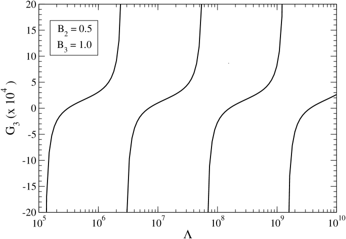
Figure 7: The dimensionless three-body coupling $G_{3}$ as a function of the cutoff $\Lambda$ for $B_{2}=0.5$ and $B_{3}=1.0$. The limit-cycle behavior of $G_{3}$ is evident from the fact that it is periodic in $\ln(\Lambda)$.

It is shown above that $h_{2}$ has no effect on the binding energies to leading order, but it does affect $G_{3}$. In fact, Eq. (130) explicitly exhibits such dependence. In Figure 8 we illustrate the effect on $G_{3}$ of changing $h_{2}$. The limit cycle behavior persists and the curves are simply distorted by the presence of non-zero $h_{2}$. Again, this behavior has been studied for many cases Mohr03 .

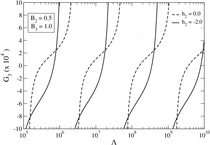
Figure 8: The dimensionless three-body coupling $G_{3}$ as a function of the cutoff $\Lambda$ for $B_{2}=0.5$ and $B_{3}=1.0$ with two different values of $h_{2}$.

XII Conclusions

We reduce the equation for S-wave bound states of three bosons interacting via attractive short range two-body interactions to a set of coupled integral equations and develop numerical methods that enable us to solve for both eigenvalues and pseudo-wave functions with a precision of 11-12 digits. This problem must be regulated (a Gaussian cutoff here to achieve high numerical precision) and renormalization produces a well-defined infinite cutoff limit (i.e., a continuum limit) if a three-body contact term is introduced with its coupling precisely tuned to a limit cycle.

The method of uniformly valid expansion is developed to separate widely different regions of momenta as a first step towards isolating and then controlling the high momentum region. We believe that this method will have applications in other renormalization problems since it addresses a generic need, but our focus is the renormalization of the three-body problem.

Unusually high precision is required because this renormalization problem is intrinsically nonperturbative and must be solved numerically at this time. We must isolate effects that scale as mixed powers of ${\rm ln}(\Lambda)$ and $1/\Lambda^{2}$ and this places stringent requirements on numerical renormalization if one needs to accurately resolve even a few levels of detail. Irrelevant operators should enable us to control these sub-leading corrections with a finite number of couplings, if we can identify appropriate irrelevant operators. It is simplest to assume that we can employ irrelevant operators from free field theory (i.e., powers of derivatives acting on regulated delta-functions for the few-body problem) but this needs to be demonstrated numerically.

Renormalization replaces an infinite geometric tower of bound states with effective interactions as the cutoff decreases. Irrelevant operators must allow us to maintain the least bound states of this tower as the cutoff descends. Our leading-order calculations show how high-momentum effects are funneled through an intermediate-momentum shell to produce a cutoff-independent tower of bound states that is entirely determined (with the two-body interaction fixed) by a single three-body coupling. The uniformly valid expansion provides a tool that should expose this structure at arbitrarily high levels of precision while providing direct insights into coupling between widely separate scales.

The three-body bound state problem we study has a rich history and many interesting current applications. The continuum limit of this problem is solved with high precision and the groundwork is laid for the next step of modulating residual cutoff dependence so that this model can be applied further.

- (1) L.H. Thomas, Phys. Rev. 47, 903 (1935).
- (2) V. Efimov, Phys. Lett. 33B, 563 (1970).
- (3) V. N. Efimov, Sov. J. Nucl. Phys. 12, 589 (1971) [Yad. Fiz. 12, 1080 (1970)].
- (4) S. Albeverio, R. Hoegh-Krohn, and T.S. Wu, Phys. Lett. 83A, 105 (1981).
- (5) P. F. Bedaque, H.-W. Hammer, and U. van Kolck, Phys. Rev. Lett. 82, 463 (1999) [arXiv:nucl-th/9809025].
- (6) P. F. Bedaque, H.-W. Hammer, and U. van Kolck, Nucl. Phys. A 646, 444 (1999) [arXiv:nucl-th/9811046].
- (7) P. F. Bedaque, H.-W. Hammer, and U. van Kolck, Nucl. Phys. A 676, 357 (2000) [arXiv:nucl-th/9906032].
- (8) K.G. Wilson, A limit cycle for three-body short range forces, talk presented at the INT program “Effective Field Theories and Effective Interactions”, Institute for Nuclear Theory, Seattle (2000); unpublished.
- (9) K.G. Wilson, Phys. Rev. D 3, 1818 (1971).
- (10) S. D. Glazek and K. G. Wilson, Phys. Rev. Lett. 89, 230401 (2002) [arXiv:hep-th/0203088].
- (11) E. Braaten and H. W. Hammer, arXiv:cond-mat/0410417 (2004).
- (12) M. Gell-Mann and F.E. Low, Phys. Rev. 95, 1300 (1954).
- (13) F.J. Wegner, Phys. Rev. B5, 4529 (1972); Phys. Rev. B6, 1891 (1972).
- (14) R. F. Mohr, Quantum Mechanical Three-Body Problem with Short Range Interactions, Ph. D. thesis, The Ohio State University (2003), arXiv:nucl-th/0306086.
- (15) M. C. Birse, J. A. McGovern and K. G. Richardson, Phys. Lett. B 464, 169 (1999) [arXiv:hep-ph/9807302].
- (16) D. B. Kaplan, M. J. Savage and M. B. Wise, Phys. Lett. B 424, 390 (1998) [arXiv:nucl-th/9801034].
- (17) D. B. Kaplan, M. J. Savage and M. B. Wise, Nucl. Phys. B 534, 329 (1998) [arXiv:nucl-th/9802075].
- (18) K.G. Wilson, Rev. Mod. Phys. 47, 773 (1975).
- (19) R. Jackiw, in “M. A. B. Beg Memorial Volume,” (A. Ali and P. Hoodbhoy, eds.), World Scientific, Singapore, 1991.
- (20) E. Braaten, H. W. Hammer and M. Kusunoki, Phys. Rev. A 67, 022505 (2003) [arXiv:cond-mat/0201281].
- (21) T. Barford and M. C. Birse, J. Phys. A 38, 697 (2005).
- (22) L. Platter, H.-W. Hammer, U.-G. Meißner, Phys. Rev. A 70, 052101 (2004).
- (23) E. Tadmor, SIAM Journal on Numerical Analysis 23, 1 (1986).
- (24) G.S. Danilov, Sov. Phys. JETP 13, 349 (1961) [J. Exptl. Theoret. Phys. (U.S.S.R.) 40, 498 (1961)].