Description of the ¹⁷F(p,$\gamma$)¹⁸Ne radiative capture reaction in the continuum shell model

Abstract

The shell model embedded in the continuum is applied to calculate the astrophysical S-factor and the reaction rate for the radiative proton capture reaction ¹⁷F(p,$\gamma$)¹⁸Ne. The dominant contribution to the cross-section at very low energies is due to M1 transitions $J_{i}^{\pi}=2^{+}\rightarrow J_{f}^{\pi}=2_{1}^{+}$ whose magnitude is controlled by a weakly bound $2_{2}^{+}$ state at the excitation energy $E_{x}=3.62$ MeV.

1 Introduction

Radiative capture reactions play a significant role in nuclear astrophysics being one of the important processes in stellar nucleosynthesis [1, 2]. Nova explosions in binary star systems occurring due to mass transfer to a white dwarf star from its companion is an important site for the CNO cycle. A thermonuclear runway results from the accreted matter accumulated on the outer layers of white dwarf star, during which ¹⁷F could be produced during hydrogen burning of the CNO elements. At this juncture the ¹⁷F(p,$\gamma$)¹⁸Ne radiative capture reaction becomes very important in deciding the fate of ¹⁷F and the subsequent routes of nucleosynthesis. The proton capture rate of ¹⁷F is also important because in competition with the ¹⁷F-$\beta$-decay rate it can provide an alternate path from the hot CNO cycle to the rapid proton (rp) burning process via the ¹⁴O($\alpha$,p)¹⁷F(p,$\gamma$)¹⁸Ne($\beta^{+},\nu$) ¹⁸F(p,$\gamma$)¹⁹Ne reaction sequence. A smaller ¹⁷F(p,$\gamma$)¹⁸Ne reaction rate compared to the ¹⁷F-$\beta$-decay rate at characteristic nova temperature and densities would favour ¹⁵O enrichment via the reaction sequence ¹⁷F($\beta^{+},\nu$)¹⁷O(p,$\alpha$)¹⁴N(p,$\gamma$)¹⁵O, whose $\beta$-decay to ¹⁵N could be an explanation for the overabundance of ¹⁵N in nova ejecta. On the other hand a large ¹⁷F(p,$\gamma$)¹⁸Ne reaction rate would alter the ¹⁸F/¹⁷F abundance ratio due to the activation of the ¹⁷F(p,$\gamma$)¹⁸Ne($\beta^{+},\nu$)¹⁸F reaction chain. A good knowledge of the ¹⁷F(p,$\gamma$)¹⁸Ne reaction rate is also thought to be important for understanding the astrophysical phenomenon of x-ray bursts.

It was first predicted in Ref. [3] that the $3^{+}$, strong $s$-wave resonance in ¹⁸Ne would occur at an excitation energy $E_{x}=4.328$ MeV with the width $\Gamma=5$ keV. This low energy $3^{+}$ was expected to substantially contribute to the ¹⁷F(p,$\gamma$)¹⁸Ne reaction rate above stellar temperatures greater than 0.2 GK, which would be important for nova explosions. Since then there have been several attempts [4, 5, 6] to experimentally measure the exact position of the $3^{+}$ level in ¹⁸Ne and it was only recently [7, 8] that this has been unambiguously put at an excitation energy $E_{x}=4.524$ MeV (center of mass energy (c.m.) $E_{r}=600$ keV) and width $\Gamma=18$ keV.

The direct capture part of the ¹⁷F(p,$\gamma$)¹⁸Ne reaction has been studied largely in a potential model framework following mainly the work of Rolfs [9]. A more microscopic approach was the extended two-cluster model (ETCM) [10], using the generator coordinate method, which has also been applied to neutron rich Carbon isotopes [11]. One of the main advantages of this method is that the resonant and non-resonant part of the reaction need not be calculated separately. However the configuration space which is used to describe the many-body states is restricted to a few cluster configurations.

Weakly bound states or resonances cannot be described in the closed quantum system (CQS) formalism [12]. For bound states, there appears a virtual scattering into the continuum phase space involving intermediate scattering states. Continuum coupling of this kind affects also the effective nucleon-nucleon interaction. For unbound states, the continuum structure appears explicitly in the properties of those states.

The importance of the particle continuum was discussed in the early days of the multiconfigurational Shell Model (SM). However, a unified description of nuclear structure and nuclear reaction aspects became possible in realistic situations only recently in the framework of the Shell Model Embedded in the Continuum (SMEC) [13, 14] which considers the nucleus as a quantum many-body system coupled to the environment of decay channels (the open quantum system (OQS) formalism). In the SMEC, all couplings involving discrete states and scattering states are calculated using the SM interaction. Inclusion of the coupling between discrete and scattering states leads to a non-hermiticity of a many-body Hamiltonian that consists of the closed system with discrete eigenstates (the standard SM Hamiltonian), and the coupling between the closed system Hamiltonian and its environment of one-nucleon [13] and two-nucleon [15, 16] decay channels. Above the particle-emission threshold, the eigenvalues of the OQS are complex. Different continuum shell-model approaches [17, 18, 19, 20], including the SMEC [13, 14, 16], are formulated in the Hilbert space, i.e., they are based on the completeness of a single-particle (s.p.) basis consisting of bound orbits and a real continuum. A different approach to the treatment of particle continuum is proposed in the Gamow Shell Model [21], which is the multi-configurational SM with a s.p. basis given by the Berggren ensemble [22] consisting of Gamow (or resonant) states and the complex non-resonant continuum of scattering states. Gamow states and the GSM can be formulated rigorously in the rigged Hilbert space (see Ref. [23] and references quoted therein).

In this work we present a study of the ¹⁷F(p,$\gamma$)¹⁸Ne radiative capture reaction using the formalism of SMEC [13, 14]. This formalism has been applied before to describe the structure of mirror nuclei ⁸B,⁸Li, and capture cross sections for mirror reactions ⁷Be(p,$\gamma$)⁸B, ⁷Li(n,$\gamma$)⁸Li [13, 24] as also to the description of ¹⁶O(p,$\gamma$)¹⁷F and ¹⁶O(p,p)¹⁶O reactions [25, 26]. The paper is organized in the following way. In section 2, we present a brief description of the SMEC formalism emphasising those aspects of the SMEC which imply the modification of the CQS eigenvalues and eigenfunctions and attempts to put the theory of nuclear structure and reactions on the same footing. We also indicate and give the relevant formulae to calculate radiative capture cross sections from both the ground state (g.s.) and excited states of the target nucleus, with properly antisymmetrized wave functions being used in both initial and final states. Section 3 contains the results and discussions of SMEC calculations of the radiative capture reaction ¹⁷F(p,$\gamma$)¹⁸Ne. The self-consistent potential, entering the coupled-channel (CC) equations of SMEC , and the parameters of the density-dependent residual interaction are presented in section 3.1. The spectrum of ¹⁸Ne obtained both in the SM and the SMEC is in section 3.2. The next two subsections 3.3 and 3.4 contain the astrophysical $S$-factors and the reaction rates of the ¹⁷F(p,$\gamma$)¹⁸Ne reaction, respectively. Finally the summary and conclusions are presented in section 4.

2 Formalism

2.1 Shell Model Embedded in the Continuum

A unified description of interdependent nuclear structure and nuclear reactions is attempted in SMEC by using a projection operator technique [27]. For the purpose of describing the one-nucleon capture reactions, we assume that the Hilbert space is decomposed into two subspaces $Q$ and $P$:

$$P+Q=I_{d}$$ (1)

The $Q$ subspace consists of $A$ particles in many-body localized states which are built up by the bound state s.p. wave functions and the part of s.p. resonance wave functions localized inside the nucleus, i.e. before a cutoff radius $R_{cut}$. The $P$ subspace contains $(A-1)$-particle states in localized states built up from (quasi-)bound single particle (qbsp) orbits and one nucleon in the scattering state. The rest of the s.p. resonant wave function (the $Q$ subspace contains the part $r<R_{cut}$ of the resonance wave function) outside the cutoff radius $R_{cut}$ are included in the $P$ subspace. The wave functions in $Q$ and $P$ are then renormalized in order to ensure their orthogonality in both subspaces. The fully antisymmetrized wave function can then be used to study the radiative capture processes where the capture can occur from both the g.s. and the excited state of the target nucleus $A-1$. This method is also fully symmetric in treating the resonant and non-resonant part of the reaction and one does not need to calculate them separately.

The first step in SMEC involves the generation of localized states in the $Q$ subspace without any coupling to the continuum. This involves solving the standard eigenvalue problem:

$$H_{QQ}\Phi_{i}=E_{i}\Phi_{i}$$ (2)

where $H_{QQ}\equiv QHQ$ is identified with the SM Hamiltonian and $\Phi_{i}$ are the localized many-body wave functions with eigenenergies $E_{i}$.

The second step consists of solving the CC equations:

$$(E^{(+)}-H_{PP})\xi_{E}^{c(+)}=0$$ (3)

where $H_{PP}=PHP$ and ${}^{\prime}+^{\prime}$ stands for the outgoing boundary conditions. The index $c\equiv(I_{t},l,s,j)$ denotes different channels characterized by $I_{t}$, the spin of the $(A-1)$ system, $s$, $l$ and $j$ which are the spin, orbital angular momentum and the total angular momentum, respectively, of the particle in the continuum. In a more explicit manner, eq. (3) is written as [14]:

$$\sum_{c^{{}^{\prime}}}(E^{(+)}-H_{cc^{{}^{\prime}}}){\xi}_{E}^{c^{{}^{\prime}}(+)}=0$$ (4)

where

$$H_{cc^{{}^{\prime}}}=(T_{kin}+U){\delta}_{cc^{{}^{\prime}}}+{\upsilon}_{cc^{{}^{\prime}}}^{J}$$ (5)

In the above equation, $T_{kin}$ stands for the kinetic-energy operator and $U$ is the finite-depth potential of Woods-Saxon (WS) type with the spin-orbit term:

$$U(r)=V_{0}f(r)+V_{SO}(4{\bf l}\cdot{\bf s})\frac{1}{r}\frac{df(r)}{dr}+V_{C}$$ (6)

where

$$f(r)=\left[1+\exp\left(\frac{r-R_{0}}{a}\right)\right]^{-1}$$ (7)

with the Coulomb potential $V_{C}$ calculated for a uniformly charged sphere of radius $R_{0}$. ${\upsilon}_{cc^{{}^{\prime}}}^{J}$ in (5) is the channel-channel coupling generated by the residual interaction between the $Q$ and $P$ subspaces and depends on the target states of the $(A-1)$ system, s.p. orbitals $l,j$ and total angular momentum and parity $J^{\pi}$ of the $A$-particle system. The explicit formulae for $H_{cc^{{}^{\prime}}}$ and ${\upsilon}_{cc^{{}^{\prime}}}^{J}$ is given in Ref. [13]. As a residual coupling between the $Q$ and $P$ subspaces, we take the density-dependent contact force [28]:

$$H_{PQ}=\nu\{\rho(r){\hat{v}}_{00}^{in} + [1-\rho(r)]{\hat{v}}_{00}^{ex}$$ (8)

$$+ {\bf\tau}_{1}.{\bf\tau}_{2}[\rho(r){\hat{v}}_{01}^{in}+[1-\rho(r)]{\hat{v}}_{01}^{ex}]\}\delta({\bf r}_{1}-{\bf r}_{2})$$

where $\nu$ is the relative strength parameter and $\rho(r)$ is the nuclear density having a Fermi form:

$$\rho(r)=\left[1+\exp\left(\frac{r-r_{n}}{d}\right)\right]^{-1}$$ (9)

with $r_{n}$ and $d$ defining the size and surface thickness of the nucleus, respectively. The values taken for the parameters are mentioned in the next section.

The diagonal part of ${\upsilon}_{cc^{{}^{\prime}}}^{J}$ changes the average potential $U$ and consequently the s.p. wave functions. So a self-consistent procedure is adopted to calculate the wave functions of those s.p. states which are occupied in the target nucleus. This iterative procedure yields a new self-consistent average potential:

$$U^{(sc)}(r)=U(r)+{\upsilon}_{cc}^{J(sc)}(r)$$ (10)

which is used to solve eq. (4).

The third system of equations:

$$(E^{(+)}-H_{PP}){\omega}_{i}^{(+)}=H_{PQ}{\Phi}_{i}\equiv w_{i}$$ (11)

defines the functions ${\omega}_{i}$ that describe the continuation of the SM states $\Phi_{i}$ into the continuum. The source term $w_{i}$ couples the wave function of the $Q$ subspace with those of the $P$ subspace.

Eigenstates of the CQS coupled to the external environment of decay channels are found by solving the eigenvalue problem for the effective Hamiltonian:

$$H_{QQ}^{eff}(E)=H_{QQ}+H_{QP}G_{P}^{(+)}(E)H_{PQ}$$ (12)

in the function space ($Q$) of the discrete states. $G_{P}^{(+)}(E)$  is the Green function for the motion of a s.p. in the $P$ subspace and is given by:

$$G_{P}=P(E-H_{PP})^{-1}P~{}\ .$$

The SM Hamiltonian $H_{QQ}$ is hermitian. On the contrary, $H_{QQ}^{eff}$ is an energy dependent, non-hermitian (complex and symmetric matrix) operator above the particle emission threshold and a hermitian (real) operator below the emission threshold. The $Q-P$ coupling contained in $H_{QQ}^{eff}$ introduce an external mixing of SM states (eigenstates of $H_{QQ}$) via the coupling to the decay channels. Diagonalization of $H_{QQ}^{eff}$ by the orthogonal but in general non-unitary transformation:

$${\Phi}_{i}\longrightarrow{\tilde{\Phi}_{j}}={\sum}_{i}b_{ji}{\Phi}_{i}$$ (13)

yields complex eigenvalues ${\tilde{E_{i}}}-\frac{1}{2}i{\tilde{{\Gamma}_{i}}}$ , which depend on the energy $E$ of the particle in the continuum. The coefficients $b_{ji}$ in (13) form a complex matrix of eigenvectors in the SM basis satisfying

$$\sum_{k}b_{jk}b_{ik}=\delta_{ji}$$ (14)

The eigenvalues of $H_{QQ}^{eff}(E)$  at energies $\tilde{E_{i}}(E)=E$, determine the energies and widths, ${\tilde{{\Gamma}_{i}}}$, of resonance states.

The total wave function, ${\Psi}_{E}^{c(c_{0})}$, for the many-body problem is now obtained in terms of ${\Phi}_{i}$ , ${\xi}_{E}^{c}$ , ${\omega}_{i}$ and the eigenvalues of $H_{QQ}^{eff}$ as:

$${\Psi}_{E}^{c(c_{0})}={\xi}_{E}^{c(c_{0})}+\sum_{i}{\tilde{\Omega}_{i}}\frac{1}{E-{\tilde{E}_{i}}+(i/2){\tilde{\Gamma}_{i}}}\langle{\tilde{\Phi}_{i}}\mid H\mid{\xi}_{E}^{c(c_{0})}\rangle$$ (15)

with the incoming wave only in channel $c_{0}$ as indicated by the superscript, and

$${\tilde{\Omega}_{i}}={\tilde{\Phi}_{i}}+{\tilde{\omega}_{i}}=(1+G_{P}^{(+)}H_{PQ}){\tilde{\Phi}_{i}}$$ (16)

with ${\tilde{\omega}_{i}}$ defined by $G_{P}^{(+)}H_{PQ}{\tilde{\Phi}_{i}}$. It is to be noted here that the SMEC formalism is fully symmetric in treating the continuum and bound state parts of the solution: ${\Psi}_{E}^{c(c_{0})}$ represents the continuum state modified by the discrete states and ${{\tilde{\Omega}}}_{i}$ represents the discrete state modified by coupling to the embedding continuum states.

The asymptotic conditions of Eq. (15) have been analyzed in Ref. [17]. One can then calculate the amplitude of the partial decay width as:

$${{\tilde{\gamma}}_{i}^{c}}={\sqrt{2\pi}}\left({{4m_{r}}\over{\hbar^{2}k_{c}}}\right)^{1/2}\sum_{j}b_{ji}\sum_{c^{\prime}}\int^{\infty}_{0}dr{\xi}_{E}^{c^{\prime}(c)}(r)w_{j}^{c^{\prime}}(r)$$ (17)

Using the proportionality relation between the matrix elements in Eq. (15) and the amplitudes of the partial widths (eq. (17)), one can derive the scattering matrix ($S$-matrix):

$$S_{c(c_{0})}=S_{c(c_{0})}^{0}-i\sum_{j}\frac{{{\tilde{\gamma}}_{j}^{c}}{{\tilde{\gamma}}_{j}^{c_{0}}}}{E-{\tilde{E}_{j}}+(i/2){\tilde{\Gamma}_{j}}}$$ (18)

In the above equation $S_{c(c_{0})}^{0}$ is determined from the asymptotic, large distance behaviour of ${\xi}_{E}^{c(c_{0})}$. The amplitudes of the partial widths ${{\tilde{\gamma}}_{j}^{c}}$ as well as the complex eigenvalues ${\tilde{E}_{j}}-(i/2){\tilde{\Gamma}_{j}}$ of the effective Hamiltonian $H_{QQ}^{eff}$ which enter in the $S$-matrix, are energy dependent. ${{\tilde{\gamma}}_{j}^{c}}$ are also complex due to the channel-channel coupling and the external mixing of SM eigenstates via the coupling to the continuum. The partial width for channel $c$ can then be defined by $\Gamma_{j}^{c}=\mid\gamma_{j}^{c}\mid^{2}$, though the total width is no longer a sum of partial widths [29]:

$$\sum_{c}\mid\gamma_{j}^{c}\mid^{2}={{\tilde{\Gamma}}_{j}}\sum_{j}\mid b_{ji}\mid^{2}\geq{{\tilde{\Gamma}}_{j}}$$ (19)

This is because the complex eigenvectors $b_{ji}$ are normalized in the sense of eq. (14), which implies:

$$\sum_{j}\mid b_{ji}\mid^{2}\geq 1$$ (20)

and which again is a direct consequence of the non-hermitian nature of the effective Hamiltonian $H_{QQ}^{eff}$ in $Q$.

Thus the formalism of SMEC provides a way to describe nuclear structure and reactions in a single framework starting from the same Hamiltonian. In the next sub-section we shall use the total wave function (15) to describe the radial part of the initial state wave function in a radiative capture process. More details about SMEC with one particle in the continuum, and general discussions about the OQS could be found in Ref. [14].

2.2 Radiative capture

We now give the general formulae to calculate radiative capture cross sections from both the g.s. and excited states of the target nucleus, with antisymmetrized wave functions used in both initial and final states. We shall apply this to the reaction ¹⁷F(p,$\gamma$)¹⁸Ne, where the proton capture can occur from both $I_{t}=5/2^{+}$ g.s. and $I_{t}=1/2^{+}$ first excited state of the target nucleus, which is ¹⁷F here.

The initial wave function $\Psi_{i}$ of the system [¹⁷F + ${\rm p}]^{J_{i}^{\pi}}$ is:

$$\Psi_{i}(r)=\sum_{l_{a},j_{a},I_{t}}i^{l_{a}}{\Psi^{J_{i}}_{l_{a},j_{a},I_{t}}(r)\over{k_{a}r}}\left[(Y^{l_{a}}\otimes\chi^{s})^{j_{a}}\otimes\chi^{I_{t}}\right]^{J_{i}}_{m_{i}}$$ (21)

where $\Psi^{J_{i}}_{l_{a},j_{a},I_{t}}(r)$ describes the radial part of the wave function (15) with one particle in the continuum. The total angular momentum in the initial channel, $J_{i}$, is the result of coupling the target spin $I_{t}$ with the total angular momentum $j_{a}$ being carried by the projectile which itself is obtained by coupling the intrinsic spin $s$ of the projectile and its relative orbital angular momentum $l_{a}$.

The final wave function $\Psi_{f}$ for the [¹⁸Ne]${}^{J_{f}^{\pi}}$ coupled to the final state total angular momentum, $J_{f}$, is:

$$\Psi_{f}(r)=\sum_{l_{b},j_{b},I_{t_{b}}}A^{j_{b}I_{t_{b}}J_{f}}_{l_{b}sj_{b}}{u^{J_{f}}_{l_{b},j_{b},I_{t_{b}}}(r)\over{r}}\left[(Y^{l_{b}}\otimes\chi^{s})^{j_{b}}\otimes\chi^{I_{t_{b}}}\right]^{J_{f}}_{m_{f}}$$ (22)

where $A^{j_{b}I_{t_{b}}J_{f}}_{l_{b}sj_{b}}$ is the coefficient of fractional parentage and $u^{J_{f}}_{l_{b},j_{b},I_{t_{b}}}(r)$ is the s.p. wave in the many-body state $J_{f}$. $s,l_{b}$ and $j_{b}$ represent the spin, the orbital angular momentum and the total angular momentum of the captured nucleon (projectile), respectively and $I_{t_{b}}$ is the final state target spin. The explicit summations over the target spin state in Eqs. (21) and (22) ensures that we take into consideration the capture from the g.s. as well as the excited states of the target nuclei.

With the wave functions $\Psi_{i}(r)$ and $\Psi_{f}(r)$, we can calculate the electric transition amplitudes of multipolarity $\lambda$ as:

$$T^{E\lambda} = C(E\lambda)i^{l_{a}}{\hat{J}}_{f}{\hat{l}}_{b}{\hat{j}}_{b}{\hat{j}}_{a}\langle\lambda\theta J_{f}m_{f}|J_{i}m_{i}\rangle\langle l_{b}0\lambda 0|l_{a}0\rangle$$ (23)

$$\times W(j_{b}I_{t}\lambda J_{i};J_{f}j_{a})W(l_{b}s\lambda j_{a};j_{b}l_{a})\delta_{I_{t}I_{t_{b}}}I^{\lambda,J_{i}}_{l_{a}j_{a},l_{b}j_{b}}$$

and the magnetic dipole transition as:

$$T^{M1} = i^{l_{a}}\mu_{N}{\hat{J}}_{f}\langle 1\theta J_{f}m_{f}|J_{i}m_{i}\rangle\{W(j_{b}I_{t}1J_{i};J_{f}j_{a}){\hat{j}}_{a}{\hat{j}}_{b}$$ (24)

$$\times\left[\mu({Z_{t}\over m_{t}^{2}}+{Z_{a}\over m_{a}^{2}}){\hat{l}}_{a}{\tilde{l}}_{a}W(l_{b}s1j_{a};j_{b}l_{a})+(-1)^{j_{b}-j_{a}}2g_{a}{\hat{s}}{\tilde{s}}W(sl_{b}1j_{a};j_{b}s)\right]$$

$$+g_{t}(-1)^{J_{f}-J_{i}}{\hat{I}}_{t}{\tilde{I}}_{t}W(I_{t}j_{b}1J_{i};J_{f}I_{t})\delta_{j_{a}j_{b}}\}\delta_{l_{a}l_{b}}\delta_{I_{t}I_{t_{b}}}I^{0,J_{i}}_{l_{a}j_{a},l_{b}j_{b}}$$

In the above formulae, $\theta=m_{i}-m_{f}$, ${\hat{a}}\equiv\sqrt{(2a+1)}$, ${\tilde{a}}\equiv\sqrt{a(2a+1)}$, and

$$C(E\lambda)=\mu^{\lambda}\left({Z_{a}\over m_{a}^{\lambda}}(-)^{\lambda}{Z_{t}\over m_{t}^{\lambda}}\right)$$

$\mu$ is the reduced mass of the system, $m_{a}$ and $m_{t}$ are the masses, $Z_{a}$ and $Z_{t}$ are the charges and $g_{a}$ and $g_{t}$ are the gyromagnetic ratios of the projectile and the target, respectively. $\mu_{N}$ is the nuclear magneton and $I^{\lambda,J_{i}}_{l_{a}j_{a},l_{b}j_{b}}$, the overlap integral is given by:

$$I^{\lambda,J_{i}}_{l_{a}j_{a},l_{b}j_{b}}=\int dru^{J_{f}}_{l_{b},j_{b},I_{t_{b}}}(r)r^{\lambda}\Psi^{J_{i}}_{l_{a},j_{a},I_{t}}(r)$$

The Kronecker symbol $\delta_{I_{t}I_{t_{b}}}$ in eqs. (23) and (24), ensures that the double summation over the target spins arising from eqs. (21) and (22) is reduced to a single one (over $I_{t}$, say). The radiative capture cross-section is then expressed as:

$$\sigma^{E1,M1} = {{16\pi}\over 9}\left({\mu\over\hbar c}\right)\left({e^{2}\over\hbar c}\right)\sum_{m_{i}m_{f}}\sum_{l_{a}j_{a}l_{b}j_{b}I_{t}}{1\over{\hat{s}}{\hat{I}_{t}}}\left({k_{\gamma}^{3}\over k_{a}^{3}}\right)|T^{E1,M1}|^{2}$$ (25)

$$\sigma^{E2} = {{4\pi}\over 75}\left({\mu\over\hbar c}\right)\left({e^{2}\over\hbar c}\right)\sum_{m_{i}m_{f}}\sum_{l_{a}j_{a}l_{b}j_{b}I_{t}}{1\over{\hat{s}}{\hat{I}_{t}}}\left({k_{\gamma}^{5}\over k_{a}^{3}}\right)|T^{E2}|^{2}$$ (26)

where $k_{\gamma}$ and $k_{a}$ are the wavevectors of the emitted photon and the incoming projectile, respectively. These formulae take into account radiative capture from both the excited state and the g.s. of the target nucleus.

3 Results and discussion

In this section we shall present the SMEC results for the spectrum of ¹⁸Ne and then go on to discuss the astrophysical S-factor and the reaction rate for the ¹⁷F(p,$\gamma$)¹⁸Ne radiative proton capture reaction.

3.1 The self-consistent potential

The $Q$ subspace in SMEC is constructed by the self-consistent, iterative method which for a given initial average s.p. potential (6) and for a given residual two-body interaction between $Q$ and $P$ subspaces (8) yields the self-consistent s.p. potential depending on the s.p. wave function $l_{j}$, the total angular momentum $J$ of the $A$-nucleon system [13, 14]. The channels in $P$: $(J_{A-1}^{\pi},l_{j})^{J}$, are defined by the states $J_{A-1}^{\pi}$ of the $A-1$ system and the s.p. wave function $l_{j}$; both are coupled to $J$ in the $A$-system. The parameters for the initial potential $U(r)$ used in the calculations for the self-consistent potential $U^{sc}(r)$ are $V_{0}=56.8853$ MeV, $V_{SO}=4.9014$ MeV, $R_{0}=3.276$ fm and $a=0.58$ fm. The potential radius $R_{0}$ has been defined using the convention $R_{0}=r_{0}(A_{t}^{1/3})$, where $r_{0}=1.27$ fm and $A_{t}=A-1$ is the mass number of the target. In the self-consistent potential, we obtain the proton s.p. orbit $1s_{1/2}$ at the experimental binding energy (-2.034 MeV) of the $J^{\pi}=2_{1}^{+}$ level of ¹⁸Ne and the $0d_{5/2}$ s.p. orbit at the experimental binding energy (-3.92 MeV) of the g.s. $J^{\pi}=0_{1}^{+}$ of ¹⁸Ne. This also puts the $0p_{1/2}$ and $0f_{7/2}$ s.p. orbits at -15.3 MeV and 8.52 MeV, respectively. Another set of parameters which enter into the calculations are those of the density-dependent residual interaction (8). These are determined to be: ${\hat{v}}_{00}^{in}=53.6,{\hat{v}}_{00}^{ex}=-438.1,{\hat{v}}_{01}^{in}=160.9,{\hat{v}}_{01}^{ex}=169.9$ all in units of of MeV$\cdot$fm³, $\nu=1.374$, $r_{n}=2.64$ fm and $d=0.58$ fm, such that the experimental width [8] of the many-body state $J^{\pi}=3^{+}$ in ¹⁸Ne is reproduced.

3.2 Spectrum of ¹⁸Ne

Figure 1: The spectrum of ¹⁸Ne. For more details, see the discussion in the text.

Fig.1 presents the energy spectrum of ¹⁸Ne calculated both in SM and in SMEC using the Zuker-Buck-McGrory (ZBM) interaction [30] in the $Q$ subspace. SM results with the original ZBM force [30] are shown on the l.h.s. of Fig.1 and are labelled by ’ZBM(1969)’. With certain changes in the matrix elements of the effective interaction (cf Table 1) we generate the SM spectrum labelled by ’ZBM’. This interaction is used also to generate the SMEC spectrum (labelled ’SMEC’). The experimental energy levels (labelled ’EXP’) are plotted on the r.h.s. of Fig.1. The experimental position of the $J^{\pi}=3_{1}^{+}$ level is taken to be the reference level in the spectra. The SM energies , SMEC energy and widths, and also the experimental data are presented in Table 2.

Table 1: The antisymmetrized two-body matrix elements in ZBM (this work) which differ from the original ZBM interaction [30]. Here, $d\equiv 0d_{5/2}$ and $s\equiv 1s_{1/2}$.

Interaction	$[dd~{}dd]$	$[dd~{}dd]$	$[dd~{}dd]$	$[ds~{}ds]$	$[ds~{}ds]$
	T=1, J=0	T=1, J=2	T=1, J=4	T=1, J=2	T=1, J=3
ZBM (this work)	$-2.01$	$-1.61$	$-0.48$	$-0.57$	$0.56$
ZBM (1969)	$-2.41$	$-1.21$	$-0.08$	$-1.17$	$1.16$

Table 2: SM energies and SMEC energies and widths vs. experimental data for ¹⁸Ne. The experimental data are from: $a\equiv$ Ref. [31], $b\equiv$ Ref. [8], $c\equiv$ Ref. [5]. Energies and widths are given in keV.

State	ZBM (1969) [30]	ZBM	SMEC		Experiment
Jπ	energy	energy	energy	width	energy	width
$0^{+}$	$-5366$	$-4668$	$-4372$	—	$-3921.6\pm 4.7^{a}$	—
$2^{+}$	$-2861$	$-2345$	$-2050$	—	$-2034.3\pm 0.2^{a}$	—
$4^{+}$	$-752$	$-639$	$-482$	—	$-545.4\pm 0.2^{a}$	—
$0^{+}$	$-1529$	$-676$	$-395$	—	$-345.3\pm 2.0^{a}$	—
$2^{+}$	$-981$	$-340$	$-119$	—	$-305.2\pm 0.6^{a}$	—
$1^{-}$	$-1326$	$-644$	$65$	$\approx 0$	$595\pm 5^{b}$	$0.1\pm 0.1$
$3^{+}$	$600$	$600$	$600$	18	$600\pm 2^{b}$	$18\pm 2$
$0^{+}$	$-319$	$338$	$941$	0.91	$666\pm 5^{b}$	$1.0\pm 1.0$
$2^{+}$	$490$	$1033$	$1569$	40.2	$1182\pm 8^{c}$	$50.0\pm 10.0$
$3^{-}$	$-759$	$-235$	$425$	0.002	$1229\pm 8^{c}$	$\leq 20$
$2^{-}$	$-167$	$84$	$839$	0.104	$1530\pm 8^{c}$	$\leq 20$

3.2.1 Further effects of the continuum coupling

Figure 2: The energy dependence of the eigenvalue (both real $E_{R}$ and imaginary $\Gamma_{R}$ parts) of the effective Hamiltonian $H_{QQ}^{eff}$ for the $3_{1}^{+}$ state in ¹⁸Ne. The solid line corresponds to inclusion of couplings to both the g.s. and the first excited state in ¹⁷F, while the dashed line corresponds to the coupling to the g.s. of ¹⁷F only.

Figure 3: The same as in Fig. 2 but for the $2_{2}^{+}$ in ¹⁸Ne. For more information see the caption of Fig. 2 and the discussion in the text.

Figs. 2 and 3 show the energy dependence of the eigenvalue of the effective Hamiltonian $H_{QQ}^{eff}$ (eq. (12)) for $J^{\pi}=3_{1}^{+}$ and $2^{+}_{2}$, respectively. The purpose of these figures is not only to show the energy dependence of the eigenvalues of the effective Hamiltonian but also to point out that the continuum coupling affects both the bound and the resonant states in the energy spectra. The top half of the figure, in both cases, shows the real part ($E_{R}$) and the bottom half shows the imaginary part ($\Gamma_{R}$) of the eigenvalue as a function of the c.m. energy ($E_{CM}$). In all cases the solid line is the result which includes couplings both to the $5/2^{+}$ g.s. and to the $1/2^{+}$ excited state of ¹⁷F, while the dashed line shows the result which includes couplings from the $5/2^{+}$ g.s. only. It is interesting to note (see Fig.  2) that $E_{R}$ differs nearly by 400 keV, at the position of the $J^{\pi}=3_{1}^{+}$ resonance, for the calculation with both the g.s. and the excited state of ¹⁷F as against only with the g.s. This shows that the coupling to the excited state is essential for the description of the real part of the $J^{\pi}=3_{1}^{+}$ energy eigenvalue. The sensitivity of the width ($\Gamma_{R}$) of the $J^{\pi}=3_{1}^{+}$ state to the coupling to the excited state is rather weak at low excitation energies. At higher energies, this coupling strongly modifies the external mixing of unperturbed SM states, changing qualitatively the energy dependence of the width (see Fig. 2).

A similar inference can be drawn from the energy dependence of the eigenvalue for the $J^{\pi}=2^{+}_{2}$ state in ¹⁸Ne (see Fig.  3). Inclusion of the excited state along with the g.s. of ¹⁷F results in a difference of about 150 keV at the position of the $2^{+}_{2}$ state with respect to the calculation without the excited state of ¹⁷F. However, considering the relative energy shifts, including the coupling to the excited state seems to be more important for the $3_{1}^{+}$ than for the $2^{+}_{2}$ state. Similarly as for the $J^{\pi}=3_{1}^{+}$ state, the imaginary part of the $J^{\pi}=2_{2}^{+}$ energy eigenvalue saturates at higher $E_{CM}$ in the absence of the coupling to the excited state of ¹⁷F.

In the following, we shall study of the effect of the continuum coupling on the spectroscopic factors in the $J^{\pi}=2^{+}_{2}$ and $J^{\pi}=3^{+}_{1}$ eigenvalues of the effective Hamiltonian $H_{QQ}^{eff}$. In SMEC, the spectroscopic factor, like the expectation value of any other operator ${\hat{O}}$, can be calculated as:

$$\langle{\hat{O}}\rangle={{{\langle\tilde{\Phi}_{j}}|{\hat{O}}|{\tilde{\Phi}_{j}}\rangle}\over{{\langle\tilde{\Phi}_{j}}|{\tilde{\Phi}_{j}}\rangle}}$$ (27)

where $\tilde{\Phi}_{j}$ (cf eq. (13)) is the eigenvector of $H_{QQ}^{eff}$. For the case of the spectroscopic factor one identifies:

$${\hat{O}}=a^{\dagger}|t\rangle\langle t|a$$ (28)

where $|t\rangle$ is the target state of the $(A-1)$-system and $a^{\dagger}$ and $a$ are creation and annihilation operators, respectively.

Figure 4: $1s_{1/2}$ spectroscopic factors to the g.s. of ¹⁷F: $[^{17}{\rm F}(5/2_{1}^{+})+1s_{1/2}]\rightarrow{{}^{18}{\rm Ne}}(2_{k}^{+})$ , $(k=1,2,3)$, for $2^{+}$ states in ¹⁸Ne as calculated in SMEC (thicker lines) and SM (thinner lines). The dashed, solid and dot-dashed lines show it for $2^{+}_{1}$, $2^{+}_{2}$ and $2^{+}_{3}$ states, respectively. The change of the spectroscopic factors from the SM to SMEC values are indicated by arrows in each case at the experimental positions of these states (cf Table 2).

Figure 5: $0d_{1/2}$ spectroscopic factors to the g.s. of ¹⁷F: $[^{17}{\rm F}(5/2_{1}^{+})+0d_{5/2}]\rightarrow{{}^{18}{\rm Ne}}(2_{k}^{+})$ , $(k=1,2)$, for $2^{+}$ states in ¹⁸Ne as calculated in SMEC (thicker lines) and SM (thinner lines) . For more details, see the caption of Fig. 4 and the discussion in the text.

Figure 6: $0d_{5/2}$ spectroscopic factors to the excited $1/2_{1}^{+}$ state in ¹⁷F: $[^{17}{\rm F}(1/2_{1}^{+})+0d_{5/2}]\rightarrow{{}^{18}{\rm Ne}}(2_{k}^{+})$ , $(k=1,2,3)$ for $2^{+}$ states in ¹⁸Ne. The dashed, solid and dot-dashed lines show it for $2^{+}_{1}$, $2^{+}_{2}$ and $2^{+}_{3}$ states, respectively. SMEC values are plotted with thicker lines. For other details, see the caption of Fig. 4 and the discussion in the text.

Figure 7: $1s_{1/2}$ spectroscopic factor to the g.s. of ¹⁷F: $[^{17}{\rm F}(5/2_{1}^{+})+1s_{1/2}]\rightarrow{{}^{18}{\rm Ne}}(3_{1}^{+})$ , for $3_{1}^{+}$ state in ¹⁸Ne as calculated in SMEC (thicker line) and SM (thinner line) . The change of the spectroscopic factors from the SM to SMEC values is indicated by an arrow at the experimental position of this state (cf Table 2).

In Fig. 4, we show the $1s_{1/2}$ spectroscopic factors $[^{17}{\rm F}(5/2_{1}^{+})+1s_{1/2}]\rightarrow{{}^{18}{\rm Ne}}(2_{k}^{+})$ , $(k=1,2,3)$ in SMEC (thicker lines) for the first three $2^{+}$ states in ¹⁸Ne and compare them with those obtained in SM (thinner lines). The SMEC spectroscopic factors are energy dependent, as a consequence of the energy-dependence of $H_{QQ}^{eff}$. Fig. 4 also shows that the coupling to the continuum has an overall effect of strongly modifying the $s$-state content of the $2^{+}_{2}$ and $2^{+}_{3}$ states, increasing and decreasing them, respectively. On the contrary, the well-bound $2^{+}_{1}$ state is weakly affected by this coupling. This redistribution of SM spectroscopic factors is a clear indication of the strong mixing of a weakly bound $2_{2}^{+}$ state and a resonance $2_{3}^{+}$ due to the $Q$-$P$ continuum coupling in the channel $(5/2_{1}^{+},s_{1/2})^{2^{+}}$. One may also notice that the external mixing of $2^{+}$ SM states changes at higher energies close to the position of the $2_{3}^{+}$ resonance $(E_{r}=1.57$ MeV).

$0d_{5/2}$ spectroscopic factors $[^{17}{\rm F}(5/2_{1}^{+})+0d_{5/2}]\rightarrow{{}^{18}{\rm Ne}}(2_{k}^{+})$ , $(k=1,2)$ in SMEC and SM for the first two $2^{+}$ states in ¹⁸Ne are shown in Fig. 5. The change of the spectroscopic factors by the external mixing is here less important and involves mainly $2^{+}_{1}$ and $2^{+}_{2}$ states. For the $2^{+}_{3}$ state, the spectroscopic factors in SM and SMEC are both very similar and small.

$0d_{5/2}$ spectroscopic factors $[^{17}{\rm F}(1/2_{1}^{+})+0d_{5/2}]\rightarrow{{}^{18}{\rm Ne}}(2_{k}^{+})$ , $(k=1,2,3)$ to the excited $1/2_{1}^{+}$ state in ¹⁷F are shown in Fig. 6. The channel $(1/2_{1}^{+},d_{5/2})^{2^{+}}$ dominates here the external mixing. The energy dependence of SMEC spectroscopic factors is similar as found for $1s_{1/2}$ spectroscopic factors to the g.s. of ¹⁷F (cf Fig. 4 ). Again, the redistribution of the SM spectroscopic factors among SMEC $2^{+}$ states concerns mainly a weakly bound $2^{+}_{2}$ state and a $2^{+}_{3}$ resonance.

The continuum coupling for $2_{2}^{+}$ state, as probed by the energy dependence of its eigenvalue and the redistribution of the spectroscopic factors, goes essentially through the coupling to the channels: $(5/2_{1}^{+},s_{1/2})^{2^{+}}$ and $(1/2_{1}^{+},d_{5/2})^{2^{+}}$. The $\ell=2$ ($d$-state) coupling to the excited $1/2_{1}^{+}$ state of ¹⁷F , changes in particular the weakly bound $2_{2}^{+}$ state (cf Fig. 3). This part of the continuum coupling for $2^{+}$ states will be strongly suppressed in the one-proton capture cross-section which is sensitive mainly to low-${\ell}$ ($\ell=0,1$) values. The role of the $1/2_{1}^{+}$ state of ¹⁷F for the rate of the reaction ¹⁷F(p,$\gamma$)¹⁸Ne will be discussed in sect. 3.4.

Fig. 7 shows the $1s_{1/2}$ spectroscopic factor $[^{17}{\rm F}(5/2_{1}^{+})+1s_{1/2}]\rightarrow{{}^{18}{\rm Ne}}(3_{1}^{+})$ , as calculated in SMEC and SM. The redistribution of the $s$-state spectroscopic factors among different $3^{+}$ SM states by the continuum coupling is here small and almost independent of the total energy of the system.

3.3 The astrophysical S - factor for the ¹⁷F(${\rm p},\gamma$)${}^{18}{\rm Ne}$ reaction

We now present the astrophysical S-factor for the capture reaction from both the $5/2_{1}^{+}$ g.s. and the $1/2_{1}^{+}$ excited state of ¹⁷F. In the SMEC calculations, all relevant transitions from the initial ($J_{i}^{\pi}=1^{-},2^{-},3^{-},2^{+},3^{+}$) correlated many-body continuum states in ¹⁸Ne to the final bound states ($J_{f}^{\pi}=0^{+}_{1,2},2^{+}_{1,2},4_{1}^{+}$) appropriate for E1,M1 and E2 transitions have been included. Since the position of the negative parity states in our calculations are somewhat lower than those experimentally observed, we have shifted the position of $J_{i}^{\pi}=1^{-}$ to its experimental value and have used the same shift for all calculations involving the negative parity states.

In Fig. 8, we present the total S-factor (solid line) for the ¹⁷F(p,$\gamma$)¹⁸Ne reaction and the separate contributions: S_E1 for E1 transitions (dotted line), S_M1 for M1 transitions (dashed line) and S_E2 for E2 transitions (dot-dashed line). The S_E2 in Fig. 8, which is orders of magnitude smaller than the S_E1 and S_M1, is multiplied by 1000. Thus, S_E1 and S_M1 components determine the reaction rate for the proton capture by ¹⁷F. At low excitation energies, S${}_{M1}>$S_E1 and above the $3_{1}^{+}$ resonance the S_E1 dominates. The value of the S-factor at zero energy, $S(0)$, is 2130.29 eV-b and the slope, ${\partial S}/{\partial E_{CM}|_{E_{CM}=0}}$, is $-6.68\times 10^{-3}~{}\rm b$. For M1 transitions, we find S${}_{M1}(0)$=1441.03 eV-b and ${\partial{\rm S}_{M1}}/{\partial E_{CM}|_{E_{CM}=0}}$=-6.84$\times 10^{-3}$ b, whereas for E1 transitions we have S${}_{E1}(0)$=689.26 eV-b and ${\partial{\rm S}_{E1}}/{\partial E_{CM}|_{E_{CM}=0}}$=+2.13$\times 10^{-4}{\rm b}$.

We will now study the important contributions to the S-factor coming from E1 and M1 transitions. The contributions to the total S-factor due to transitions to the different final states of ¹⁸Ne are shown in Fig. 9. Transitions to the $J_{f}^{\pi}=2^{+}_{1}$ bound state of ¹⁸Ne dominate over all other contributions. This fact is also borne out by calculations presented in Ref. [10].

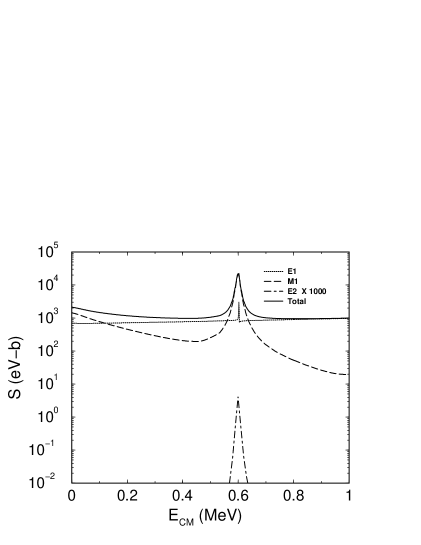
Figure 8: S-factor (solid line) for the ¹⁷F(p,$\gamma$)¹⁸Ne reaction and the total contributions from the E1(dotted line), M1(dashed line) and E2(dot-dashed line).

Figure 9: The S-factor in SMEC is shown separately for transitions to different final states of ¹⁸Ne.

Figure 10: E1 part of the S-factor and the individual contributions relevant for the ¹⁷F(p,$\gamma$)¹⁸Ne capture reaction.

Figure 11: Contributions to S_M1 from $J_{i}^{\pi}=3^{+}$ to $J_{f}^{\pi}=2^{+}_{1,2},4_{1}^{+}$ transitions in ¹⁸Ne.

Fig. 10 shows the S_E1-factor and the individual contributions relevant for the capture reaction. Since the experimental $J_{i}^{\pi}=3_{1}^{-},2_{1}^{-}$ states in ¹⁸Ne are at energies above 1 MeV, we show only their non-resonant contribution to the S_E1-factor. The non-resonant contribution from the $J_{i}^{\pi}=3^{-},2^{-}$, to $J_{f}^{\pi}=2^{+}_{1,2}$ final states are shown by thick dashed and dot-dashed lines, respectively. The contributions from the $J_{i}^{\pi}=1^{-}$ initial state to $J_{f}^{\pi}=2^{+}_{1,2}~{}{\rm and}~{}0^{+}_{1,2}$ are shown by long dashed and dotted lines, respectively. The total S_E1 is represented by the solid line. In all cases, as has been pointed out earlier, the contributions to the $J_{f}^{\pi}=2^{+}_{1}$ bound state of ¹⁸Ne dominate over all other contributions. The low energy direct part of the E1 cross-section in our calculations is less than what has been reported in Refs. [4, 10] due to a different choice of the potential radius. The physical picture in SMEC consists of generating the s.p. wave functions of the nucleon (proton) moving in the potential well created by the nucleons in the target nucleus (i.e., $R_{0}\sim 17^{1/3}$) and not in the combined well of the target nucleus and the nucleon (i.e., $R_{0}\sim(17^{1/3}+1^{1/3})$) as used in [9, 4, 10]. This physical picture has been followed in all previous SMEC studies of the radiative capture reactions [13, 25, 26], giving an excellent description of the E1 component.

Attempts to extract the direct capture cross section of the ¹⁷F(p,$\gamma$)¹⁸Ne reaction from the transfer reactions measurements are underway [32]. This procedure involves measuring the ¹⁴N(¹⁷F,¹⁸Ne)¹³C proton-transfer reaction cross section and determining the asymptotic normalization coefficients (ANC) for the ¹⁸Ne bound states from a DWBA analysis of the results. Asuming that the measured transfer reaction is peripheral, one could then relate the extracted ANC with the direct capture rate at low energies [33, 34]. Earlier applications of this method have been to the ¹⁶O(p,$\gamma$)¹⁷F [34] and ⁷Be(p,$\gamma$)⁸B [33] reactions to determine the astrophysical S-factor at low energies. Peripheral transfer reactions would be most sensitive to the tail of the wave functions beyond the range of the nuclear potential than to the inner region and hence the strength of this method is supposed to lie in the fact that the potential model bound state wave function could be well reproduced by a linearly scaled Whittaker function in the asymptotic region [35], thereby reducing the dependence on the potential parameters. However it is to be mentioned here that the low energy part of the S-factor may not be entirely due to the pure E1 component for a particular radiative capture process. Importance of this fact will become more apparent as we continue our discussions to the M1 transtions, especially on the $J_{i}^{\pi}=2^{+}$ to $J_{f}^{\pi}=2^{+}_{1,2}$ M1 transitions.

In Fig. 11, we present the contributions to S_M1 from $J_{i}^{\pi}=3^{+}$ (continuum states) to $J_{f}^{\pi}=2^{+}_{1,2},4_{1}^{+}$ (bound states) transitions in ¹⁸Ne. As remarked earlier, the transitions to the $2^{+}_{1}$ final state, shown by the solid line in Fig. 11, dominate peaking at the position of the $3_{1}^{+}$ resonance. The transitions to $2^{+}_{2}$ and to $4_{1}^{+}$ are shown by dotted and dashed lines, respectively. The proton capture from the excited state of ¹⁷F has a negligible effect on the value of S_M1. This, at first instance, may sound contradictory to the inferences from Fig. 2, where inclusion of the excited state couplings were shown to affect the energy eigenvalues. However, these couplings involve a $d$-state whose contribution to the proton capture is strongly reduced in comparison with the $s$-state contribution. The latter one is present in the radiative capture in the $5/2^{+}$ (g.s.) channel. Moreover, the $1/2^{+}$ excited channel opens at 495 keV, reducing the available energy for the proton capture and, hence, reducing importance of this channel in the proton capture cross-section, in particular at low $E_{CM}$.

Much more important contribution to S_M1 comes from transitions from the $J_{i}^{\pi}=2^{+}$ continuum to the $J_{f}^{\pi}=2^{+}_{1,2}$ bound states of ¹⁸Ne (see Fig. 12). The solid line and the dashed line show the transition to the $2^{+}_{1}$ and $2^{+}_{2}$ bound states of ¹⁸Ne, respectively. The $2^{+}$ continuum at low excitation energies is strongly correlated by the proximity of a weakly bound $2_{2}^{+}$ state which induces a resonant-like feature (’resonant-halo’) in the $2^{+}$ continuum owing to its large $s$-spectroscopic factor (cf a discussion of Fig. 4). Hence, the dominant M1 component at low energies (below 0.4 MeV) comes from the transitions between $2^{+}_{2}$-parented continuum states and the well-bound $2_{1}^{+}$ state. The weakly bound $2_{2}^{+}$ state plays in this scenario a role of the catalyzer of the proton capture reaction. At higher energies, especially in the vicinity of the $3^{+}$ resonance at 600 keV we see the dominance of $J_{i}^{\pi}=3^{+}$ to $J_{f}^{\pi}=2^{+}_{1}$ M1 transitions.

Figure 12: The M1 transitions from $J_{i}^{\pi}=2^{+}$ to $J_{f}^{\pi}=2^{+}_{1,2}$ bound states of ¹⁸Ne.

Figure 13: The S-factor for the $J_{i}^{\pi}=2^{+}$ to $J_{f}^{\pi}=2^{+}_{1}$ M1 transition at a fixed energy $\rm E_{CM}=50~{}keV$, as a function of the position ($\rm E_{2^{+}_{2}}$) of the weakly bound $2^{+}_{2}$ state in ¹⁸Ne with respect to the proton emission threshold.

For a given strength of the continuum coupling ($Q-P$ coupling) and fixed radial s.p. wave functions involved in the calculation of the source term [13, 14] (cf eq. (11)), the rate of the proton capture in M1 transitions: $J_{i}^{\pi}=2^{+}\longrightarrow J_{f}^{\pi}=2_{1}^{+}$, depends solely on the position of the $2_{2}^{+}$ state with respect to the one-proton emission threshold. In Fig. 13, we show the S_M1-factor at a fixed c.m. energy $E_{CM}=50$ keV for the $J_{i}^{\pi}=2^{+}\longrightarrow J_{f}^{\pi}=2^{+}_{1}$ transitions, as a function of the energy ($\rm E_{2^{+}_{2}}$) of the $2^{+}_{2}$ state with respect to the one-proton emission threshold. The WS potential generating the s.p. wave functions is kept fixed in these calculations (see sect. 3.1). One can see from Fig. 13 that changing the energy $E_{2_{2}^{+}}$ of the $2_{2}^{+}$ state from -400 keV to 0 (the one-proton emission threshold) changes the S_M1-factor by two orders of magnitude.

This astonishing effect is not due to an increased radial size of the s.p. orbits, in particular of the $1s$-state, involved in the $2_{2}^{+}$ state since the average potential is kept fixed for all values of $\rm E_{2^{+}_{2}}$. The effect seen in Fig. 13 is a consequence of the strong interference between $2^{+}_{2}$ and $2_{3}^{+}$ eigenvalues of the effective Hamiltonian which shifts a significant part of the $2_{3}^{+}$ resonance strength into the region of low energy continuum. This is a genuine interference effect in the OQS: states having a similar structure and coupled strongly to the environment of decay channels change in such a way that one state close to the emission threshold aligns its wave function with the decay channel, i.e. its wave function becomes more similar to the channel wave function [14, 36, 37]. A similar segregation effect has been found in Refs. [36, 37] in the distribution of widths of the resonance states. Mixing of resonances via the coupling to the decay channels leads to the so-called resonance trapping, i.e. a major part of the decay width becomes concentrated in one (or more) resonance(s) in the case of one (or more) open channel(s) if the strength of the external coupling is sufficiently strong, whereas remaining states have negligible width and, hence, are trapped. In the considered example of $2^{+}$ discrete states of ¹⁸Ne, the $1s_{1/2}$ spectroscopic amplitudes in SM states $2_{2}^{+}$ and $2_{3}^{+}$ are large, indicating a strong mutual coupling (strong external mixing) of these two many-body states via the $\ell=0$ one-particle continuum. This kind of coupling may lead to the situation that one of the $2^{+}$ eigenstates of the effective Hamiltonian closest to the one-proton emission threshold ($2_{2}^{+}$ in the studied case) increases its $s$-state content and aligns with the decay channel $[(A-1)\otimes{\rm p}]=[5/2^{+}\otimes s_{1/2}]$ at the expense of other $2^{+}$ eigenstates. The proton capture in the $s$-wave then becomes enhanced because the correlations in low-energy continuum states generated by an aligned subthreshold state become enhanced by a downwards shift of the $s$-state strength from the region of $2_{3}^{+}$ resonance. This message was also conveyed by the conclusions drawn from Fig. 4 which shows that the coupling to the continuum has the overall effect of strongly modifying the $s$-state content of the $2^{+}_{2}$ and $2^{+}_{3}$ states, and thereby redistributing their strengths.

Table 3: The $1s_{1/2}$ spectroscopic amplitudes in the $2^{+}_{2}$ state of ¹⁸Ne for different SM effective interactions.

ZBM (this work)	WBT [38]	PSDFP [15]
0.701	0.764	0.762

The effect is all the more accentuated by the large $s$-state spectroscopic amplitude in the $2_{2}^{+}$ state. To verify that this is not an artifact of the ZBM interaction, we have also shown in Table 3 the corresponding numbers for two different SM effective interactions, WBT [38] and PSDFP [15], also used for A = 18 mass region. We see that the magnitudes of the $s$-state spectroscopic amplitudes are similar for all these interactions.

3.4 The ${}^{17}{\rm F}({\rm p},\gamma)^{18}{\rm Ne}$ reaction rates

As has been mentioned earlier the radiative proton capture by ¹⁷F plays an important role in the nucleosynthesis. In Table 4, we present the reaction rate, $N_{A}\langle\sigma v\rangle$ in $\rm cm^{3}mole^{-1}s^{-1}$ for this reaction as a function of some typical stellar temperatures $T$ (in GK). $\langle\sigma v\rangle$ is the reaction rate per particle pair [39] and $N_{A}$ is Avogadro’s number. Column 1 of Table 4 shows the SMEC results calculated taking into consideration the capture from both the $5/2^{+}$ g.s. and the $1/2^{+}$ excited state of ¹⁷F, while the column designated by SMEC (g.s.) shows the result for proton capture from the $5/2^{+}$ g.s. of ¹⁷F alone. We do not see any noticeable difference in the reaction rates in these two calculations, particularly below temperatures of 0.4 GK which are more important for nova nucleosynthesis. This is understandable because the Gamow window spans lower energies at these temperatures and, moreover, the $1/2^{+}$ excited state channel involves the proton capture in the $d$-wave and is strongly disfavored by the centrifugal barrier.

The last column in Table 4 is the reaction rate from Ref. [8], which is quoted here for the purpose of comparison with our reaction rate. The SMEC rates are lower by a factor of 2-3 below 0.4 GK and by a factor of 7.5 at 2.0 GK, as compared with those of Ref. [8], primarily because of the lower E1 contributions due to the reasons mentioned in the previous section.

In Fig. 14, we show the variation of the total reaction rate as a function of temperature and for some important transitions. The total contribution is shown by the solid line, while the dotted and short-dashed lines represent the contributions from the E1 and M1 components, respectively. Amongst the M1 components the contributions from the $J_{i}^{\pi}=2^{+}$ to $J_{f}^{\pi}=2^{+}_{1,2}$ components (long-dashed) dominate the rate at lower temperatures and accounts for almost all the M1 cross-section below about 0.4 GK, while the contributions from $J_{i}^{\pi}=3^{+}$ to $J_{f}^{\pi}=2^{+}_{1,2}$ (dot-dashed) are dominant at higher temperatures.

Table 4: ¹⁷F(p,$\gamma$)¹⁸Ne reaction rates in $\rm cm^{3}mole^{-1}s^{-1}$ in SMEC and Ref.[8] for some typical stellar temperatures (in GK). For other descriptions see the text.

T($10^{9}$K)	SMEC	SMEC (g.s.)	Ref. [8]
0.1	1.317 $\times 10^{-9}$	1.317 $\times 10^{-9}$	(2.68$\pm$0.38) $\times 10^{-9}$
0.2	2.209 $\times 10^{-6}$	2.209 $\times 10^{-6}$	(5.15$\pm$0.75) $\times 10^{-6}$
0.3	7.736 $\times 10^{-5}$	7.736 $\times 10^{-5}$	(1.97$\pm$0.29) $\times 10^{-4}$
0.4	7.458 $\times 10^{-4}$	7.453 $\times 10^{-4}$	(2.29$\pm$0.40) $\times 10^{-3}$
0.5	4.124 $\times 10^{-3}$	4.116 $\times 10^{-3}$	(1.77$\pm$0.49) $\times 10^{-2}$
0.6	1.646 $\times 10^{-2}$	1.640 $\times 10^{-2}$	(9.29$\pm$3.28) $\times 10^{-1}$
0.7	5.023 $\times 10^{-2}$	5.000 $\times 10^{-2}$	(3.32$\pm$1.30) $\times 10^{-1}$
0.8	1.227 $\times 10^{-1}$	1.221 $\times 10^{-1}$	(8.80$\pm$3.61) $\times 10^{-1}$
0.9	2.516 $\times 10^{-1}$	2.503 $\times 10^{-1}$	(1.88$\pm$0.78) $\times 10^{0}$
1.0	4.516 $\times 10^{-1}$	4.491 $\times 10^{-1}$	(3.43$\pm$1.44) $\times 10^{0}$
1.5	2.643 $\times 10^{0}$	2.629 $\times 10^{0}$	(1.97$\pm$0.78) $\times 10^{1}$
2.0	6.185 $\times 10^{0}$	6.155 $\times 10^{0}$	(4.62$\pm$1.64) $\times 10^{1}$

Figure 14: The variation of the total reaction rate as a function of temperature and for some important transitions. The total reaction cross-section is shown by the solid line, while the dotted and short-dashed lines represent the E1 and M1 components, respectively. For more details, see the description in the text.

It would be interesting to investigate the astrophysical implications of our ¹⁷F(p,$\gamma$)¹⁸Ne reaction rate, especially in nova explosions. The previous reaction rates of Wiescher et al. [3] are higher than that of Bardayan et al. [8] based on the recent determination of the energy and the total width of the $J^{\pi}=3^{+}$ state in ¹⁸Ne and adding the non-resonant direct capture rate from the potential model in Ref. [4]. The reaction rates of Sherr and Fortune [40] and García et al. [4] are rather similar to those of Bardayan et al. below about 0.4 GK and are a bit lower at higher temperatures. The reaction rate of Ref. [8] was used to calculate [41] the nucleosynthesis in nova outbursts on the surfaces of 1.25 M_⊙ and 1.35 M_⊙ ONeMg white dwarfs and a 1.00 M_⊙ CO white dwarf. It was shown that for a 1.25 M_⊙ white dwarf a slower ¹⁷F(p,$\gamma$)¹⁸Ne reaction rate produced more ¹⁸F than the faster rate because the ¹⁸F (produced from the $\beta$-decay of ¹⁸Ne) at lower temperatures would survive as ¹⁸F and would not be destroyed by the ¹⁸F(p,$\alpha$)¹⁵O reaction. Although a faster ¹⁷F(p,$\gamma$)¹⁸Ne reaction rate does allow more conversion of ¹⁷F to ¹⁸F, but since this ¹⁸F would be produced at higher temperatures it would be destroyed by the ¹⁸F(p,$\alpha$)¹⁵O reaction. Thus a larger final abundance of ¹⁸F would be obtained with a slower ¹⁷F(p,$\gamma$)¹⁸Ne reaction rate. It was also calculated that for a 1.35 M_⊙ white dwarf the abundances of ¹⁷O and ¹⁷F increased by a factor of 14000, as against estimates based on rates from Ref. [3], in the third hottest zones of the nova. For a 1.00 M_⊙ CO white dwarf, which involves lower peak temperatures than the other two cases, only small variation in the mass fraction of various isotopes were observed except for ¹⁸Ne; where it increased by $21\%$ as compared to Ref. [3].

Our reaction rate is lower than those of Ref. [8] by nearly a factor of 2-3 below 0.4 GK. This is also about the temperature range of the hottest zone in 1.25 M_⊙ and 1.35 M_⊙ white dwarfs, which are 0.333 GK and 0.457 GK, respectively [41]. For a 1.25 M_⊙ white dwarf, with our lower rate, we would also qualitatively expect a large ¹⁸F abundance produced at lower temperatures and not being destroyed by the ¹⁸F(p,$\alpha$)¹⁵O reaction due to the same reasons as mentioned in the previous paragraph. The final abundances of ¹⁸F, in 1.35 M_⊙ white dwarf, could be slightly less than in Refs. [3, 41], following the same trends as in Ref. [41]. Moreover, recent measurements [42] seems to suggest that the estimated ¹⁸F(p,$\alpha$)¹⁵O reaction rate could be 2-5 times less than what was estimated in recent calculations [43, 44, 45]. This would imply the survival of ¹⁸F ($T_{1/2}=110$ min) and this opens up the possibility of detecting the characteristic 511 keV $\gamma$-ray, from the electron-positron annihilation following the $\beta$-decay of ¹⁸F, using the techniques of gamma-ray astronomy. This, in turn would provide us an opportunity to gain further insights about the nova mechanism.

Furthermore, our lower ¹⁷F(p,$\gamma$)¹⁸Ne reaction rate would allow more ¹⁷F to survive and the production of more ¹⁷O by ¹⁷F($\beta^{+},\nu$)¹⁷O in both 1.25 M_⊙ and 1.35 M_⊙ white dwarfs as compared to the values reported in [41]. Moreover, apart from the branch which produces ¹⁸F via the ¹⁷O(p,$\gamma$)¹⁸F reaction, the synthesis of ¹⁵O by the ¹⁷O(${\rm p},\alpha$)¹⁴N(${\rm p},\gamma$)¹⁵O reaction chain would be more feasible with the rates reported in this work. The $\beta$-decay of ¹⁵O to ¹⁵N could be a way of explaining the overabundance of ¹⁵N in the nova ejecta [46].

For a 1.00 M_⊙ CO white dwarf, which involves lower peak temperatures, we would generally concur with the scenario predicted in Ref. [41] as our rates would be closer to the rates of Ref. [8] at lower temperatures. We would probably have similar abundances for most of the isotopes as in Refs. [3, 41] except for abundances of ¹⁸Ne, which could be higher in our case following the similar trends as in Ref. [41].

4 Summary and conclusions

In this work, we have applied the open quantum system formalism of the SMEC for the microscopic description of the ¹⁸Ne spectra, low energy astrophysical S-factor and reaction rates for the radiative proton capture reaction ¹⁷F(p,$\gamma$)¹⁸Ne. SMEC is a model in which the realistic SM solutions for (quasi-)bound states are coupled to the environment of one-particle [13, 14] and two-particle decay channels [16] for the description of complicated low energy excitations of weakly bound nuclei and various nuclear reactions and decays involving up to two nucleons in the scattering continuum. This theoretical model, which attempts a unified description of interdependent nuclear structure and reaction theories by using a projection operator technique [27], is a recent development of the Continuum Shell Model (CSM) [17, 18, 19].

Inclusion of the target excited state was shown to have an influence on the eigenvalues of the effective Hamiltonian. It was seen that the energy of the $3^{+}$ resonance in ¹⁸Ne could be different by as much as 400 keV, depending on whether the excited state couplings were included or not. It was also interesting to observe the energy dependence of the spectroscopic factors for the first three $2^{+}$ states in ¹⁸Ne. The coupling to the continuum strongly modifies the $s$-state content of the weakly bound $2^{+}_{2}$ and resonant $2^{+}_{3}$, decreasing the latter and reinforcing the former, with respect to their SM values. On the other hand the $s$-state content of the $2^{+}_{1}$ state was not affected too much by the continuum couplings by virtue of it being well below the particle emission threshold. It would ve very nice if, in some future experiment, these spectroscopic factors could be measured, especially those of the $2^{+}_{1}$ and $2^{+}_{2}$.

We also calculated the astrophysical S-factors for the radiative capture reaction ¹⁷F(p,$\gamma$)¹⁸Ne, where the capture could occur from both the $5/2^{+}$ g.s. and the $1/2^{+}$ first excited state of ¹⁷F. Fully antisymmetrized wave functions were used in both the initial and final states of the radiative capture process. This method is also fully symmetric in treating the resonant and non-resonant part of the reaction and one does not need to calculate them separately. We have shown that in the region around 600 keV the $J_{i}^{\pi}=3^{+}$ to $J_{f}^{\pi}=2^{+}_{1}$ component of the M1 dominates the S-factor, but at very low energies (below 0.4 MeV) the M1 component arising from the $J_{i}^{\pi}=2^{+}$ to $J_{f}^{\pi}=2^{+}_{1}$ transition has a substantial impact on the low energy S-factor. In fact its contribution is even more than the E1 component below 0.1 MeV. This has been traced back to the strong mixing of the weakly bound $2^{+}_{2}$ state with the $2^{+}_{3}$ resonance in the low energy correlated $2^{+}$ continuum wave function. One should, thus be careful while analyzing the low energy direct capture part of the reaction with theories, which tend to minimize the effect of nuclear structure in nuclear reactions. It would indeed be extremely interesting if in proposed experiments [47], the low energy E1 and M1 components could be disentangled and the low energy behaviour of the M1 is studied in more details.

We have also calculated the reaction rate for the ¹⁷F(p,$\gamma$)¹⁸Ne radiative capture reaction for some typical stellar temperatures. Our rates are lower by a factor of 2-3 below 0.4 GK and by a factor of 7.5 at 2.0 GK, as compared with those of Ref. [8]. Qualitatively we predict a similar situation in novae nucleosynthesis, following the trends reported in Ref. [41], with perhaps a larger abundance of ¹⁷F and ¹⁷O. It would also be interesting to investigate if our smaller reaction rates could eventually lead to a larger ¹⁵O abundance whose $\beta$-decay to ¹⁵N could be a way of explaining the overabundance of ¹⁵N in the nova ejecta [46].

References

- [1] E. M. Burbidge, G. R. Burbidge, W. A. Fowler, and F. Hoyle, Rev. Mod. Phys. 29 (1957) 547.
- [2] C. Rolfs and C. A. Barnes, Annu. Rev. Nucl. Part. Sci. 40 (1990) 45.
- [3] M. Wiescher, J. Górres and K.-F. Thielemann, Astrophys. J. 326 (1988) 384.
- [4] A. García et al., Phys. Rev. C 43 (1991) 2012.
- [5] K. I. Hahn et al., Phys. Rev. C 54 (1996) 1999.
- [6] S. H. Park et al., Phys. Rev. C 59 (1999) 1182.
- [7] D. W. Bardayan et al., Phys. Rev. Lett. 83 (1999) 45.
- [8] D. W. Bardayan et al., Phys. Rev. C 62 (2000) 055804.
- [9] C. Rolfs, Nucl. Phys. A 217 (1973) 29.
- [10] M. Dufour and P. Descouvement, Nucl. Phys. A 730 (2004) 316.
- [11] P. Descouvement, Nucl. Phys. A 675 (2000) 559.
- [12] J. Dobaczewski and W. Nazarewicz, Phil. Trans. R. Soc. Lond. A 356 (1998) 2007.
- [13] K. Bennaceur, F. Nowacki, J. Okołowicz and M. Płoszajczak, Nucl. Phys. A 651 (1999) 289.
- [14] J. Okołowicz, M. Płoszajczak and I. Rotter, Phys. Rep. 374 (2003) 271.
- [15] J. Rotureau, J. Okołowicz and M. Płoszajczak, Acta Phys. Pol. B 35 (2004) 1283.
- [16] J. Rotureau, J. Okołowicz and M. Płoszajczak, Phys. Rev. Lett. 95 (2005) 042503.
- [17] H. W. Bartz, I. Rotter and J. Höhn, Nucl. Phys. A 275 (1977) 111.
- [18] H. W. Bartz, I. Rotter and J. Höhn, Nucl. Phys. A 307 (1977) 285.
-
[19]
H. R. Kissener, I. Rotter and N. G. Goncharova, Fortschr. Phys.
35 (1987) 277;
I. Rotter, Rep. Prog. Phys. 54 (1991) 635. -
[20]
A. Volya and V. Zelevinsky, Phys. Rev. C 67 (2003) 054322;
A. Volya and V. Zelevinsky, Phys. Rev. Lett. 94 (2005) 052501. -
[21]
N. Michel, W. Nazarewicz, M. Płoszajczak and K. Bennaceur, Phys. Rev. Lett. 89 (2002) 042502.;
N. Michel, W. Nazarewicz, M. Płoszajczak and J. Okołowicz, Phys. Rev. C 67 (2003) 054311;
R. Id Betan, R.J. Liotta, N. Sandulescu and T. Vertse, Phys. Rev. Lett. 89 (2002) 042501;
R. Id Betan, R.J. Liotta, N. Sandulescu and T. Vertse, Phys. Rev. C 67 (2003) 014322. -
[22]
T. Berggren, Nucl. Phys. A 109 (1968) 265;
T. Berggren and P. Lind, Phys. Rev. C 47 (1993) 768;
P. Lind, Phys. Rev. C 47 (1993) 1903. - [23] O. Civitarese and M. Gadella, Phys. Rep. 396 (2004) 41.
- [24] K. Bennaceur, F. Nowacki, J. Okołowicz and M. Płoszajczak, J. Phys. G 24 (1998) 1631.
- [25] K. Bennaceur et al., Phys.Lett. B 488 (2000) 75.
- [26] K. Bennaceur, F. Nowacki, J. Okołowicz and M. Płoszajczak, Nucl. Phys. A 671 (2000) 203.
- [27] H. Feshbach, Ann. Phys. (N.Y.) 5 (1958) 357; ibid 19 (1962) 287.
- [28] B. Schwesinger and J. Wambach, Nucl. Phys. A 426 (1984) 253.
- [29] C. Mahaux and H. Wiedenmüller, Shell Model approach to Nuclear Reactions, North-Holland, Amsterdam (1969).
-
[30]
A. P. Zuker, Phys. Rev. Lett. 23 (1969) 983.
A. P. Zuker, B. Buck and J.B. McGrory Phys. Rev. Lett. 21 (1968) 39. - [31] D. R. Tilley, H. R. Weller, C. M. Cheves and R. M. Chasteler, Nucl. Phys. A 595 (1995) 1.
- [32] J. C. Blackmon et al., Nucl. Phys. A 718 (2003) 587c; ibid. 746 (2004) 365c.
- [33] H. M. Xu et al., Phys. Rev. Lett. 73 (1994) 2027.
- [34] C. A. Gagliardi et al., Phys. Rev. C 59 (1999) 1149.
- [35] A. M. Mukhamedzhanov et al., Phys. Rev. C 56 (1997) 1302.
-
[36]
P. Kleinwa̋chter and I. Rotter, Phys. Rev. C 32 (1985) 1742;
W. Iskra, M. Müller, and I. Rotter, J. Phys. G 19 (1993) 2045. - [37] S. Drożdż, J. Okołowicz, M. Płoszajczak and I. Rotter, Phys. Rev. C 62 (2000) 24313.
- [38] E.K. Warburton and B.A. Brown, Phys. Rev. C 46 (1992) 923.
- [39] C. E. Rolfs and W. S. Rodney, Couldrons in the Cosmos (University of Chicago Press, Chicago 1988).
- [40] R. Sherr and H. T. Fortune, Phys. Rev. C 58 (1998) 3292.
- [41] S. Parete-Koon et al., Astrophys. J. 598 (2003) 1239; arXiv: astro-ph/0308216.
- [42] R. L. Kozub et al., Nucl. Phys. A 758 (2005) 753c; Phys. Rev. C 71 (2005) 032801(R).
- [43] A. Coc et al., Astron. Astrophys. 357 (2000) 561.
- [44] D. W. Bardayan et al., Phys. Rev. Lett. 89 (2002) 262501.
- [45] N. de Séréville et al., Phys. Rev. C 67 (2003) 052801(R).
- [46] Y. Chin, C. Henkel, N. Langer and R. Mauersberger, Astrophys. J. Lett. 512 (1999) L143.
- [47] R. Fitzgerald et al., Nucl. Phys. A 748 (2005) 351.