Abstract

The gap equation in the ${}^{1}S_{0}$-channel is solved for a nuclear slab with the separable form of the Paris potential. The gap equation is considered in the model space in terms of the effective pairing interaction which is found in the complementary subspace. The absolute value of the gap $\Delta$ turned out to be very sensitive to the cutoff $K_{max}$ in the momentum space in the equation for the effective interaction. It is necessary to take $K_{max}{=}160\div 180\;$fm^-1 to guarantee 1% accuracy for $\Delta$. The gap equation itself is solved directly, without any additional approximations. The solution reveals the surface enhancement of the gap $\Delta$ which was earlier found with an approximate consideration. A strong surface-volume interplay was found also implying a kind of the proximity effect. The diagonal matrix elements of $\Delta$ turned out to be rather close to the empirical values for heavy atomic nuclei.

1 Introduction

The microscopic theory of nuclear pairing is yet far from being complete. Some progress was achieved only recently. In a series of papers (see [1] and Refs. therein), the problem was attacked within a two-step approach in which the full Hilbert space of the problem $S$ is split into the model subspace $S_{0}$ and the complementary one, $S^{\prime}$. The gap equation should be solved in the model space in terms of the effective pairing interaction (EPI) $V^{p}_{\mbox{\scriptsize eff}}$ which obeys the Bethe-Goldstone-type equation in the complementary subspace. The pairing effects could be neglected in the latter provided the model space is sufficiently wide. The simplest nuclear systems with one-dimensional (1D) inhomogeneity were considered, i.e. semi-infinite nuclear matter and the nuclear slab. These simplifications permitted to find the EPI directly without additional approximations for the separable representation [2, 3] of the Paris NN-potential [4]. To save the computing time, it was suggested also an approximate method of finding the EPI, the so-called local-potential approximation (LPA), which has very high accuracy [1].

At the same time, the gap equation in [1] was solved only approximately, with the help of a generalization to non-homogeneous systems of the method by V.A. Khodel, V.V. Khodel and J.W. Clark (KKC) [5]. Here we report the result of the direct solution of the gap equation for the nuclear slab system.

In recent quite relevant paper by F. Barranco et al. [6], the direct solution of the gap equation for a finite nucleus (¹²⁰Sn) was carried out for the realistic Argonne $v14$ NN-potential. It yielded the gap $\Delta$ which is about a half of the experimental value. The lack of the gap was attributed in [6] to the contribution of the low-lying surface vibrations. Comparison of the results of our calculation with those of Ref. [6] will show to what extent the predictions of the microscopic calculation of $\Delta$ in finite systems depend on the form of the realistic NN-potential and other details. In particular, it is well known [7] that the gap value in infinite matter is rather sensitive to the value of the effective mass $m^{*}$. It is illustrated with Fig. 1 for the case of the Paris NN-potential. Qualitatively, such a strong dependence of $\Delta$ could be explained by the simplest BCS formula for $\Delta$ in the case of the momentum independent force:

$$\Delta=\varepsilon_{0}\exp\left(-\frac{m}{m^{*}g}\right),$$ (1)

where $g$ is the dimensionless effective pairing interaction strength, and the energy coefficient $\varepsilon_{0}$ depends on the cutoff in the integral over momentum in the BCS gap equation.

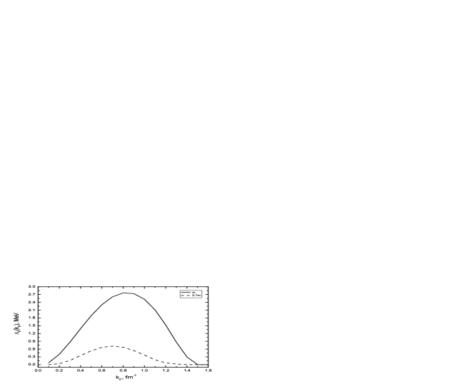
Figure 1: The gap $\Delta_{\mbox{\scriptsize F}}(k_{\mbox{\scriptsize F}})$ in nuclear matter for Paris force. The solid line corresponds to the effective mass $m^{*}=m$, the dashed one, to $m^{*}=0.7m$.

In [6] the coordinate dependent effective mass $m^{*}(r)$ was used of the Sly4 version [8] of the Skyrme force. Its value changes from $m^{*}=0.7m$ inside a nucleus to $m^{*}=m$ outside. We prefer to deal with the prescription of $m^{*}=m$ which is closer to the “experimental” nuclear value. The latter was found in Ref. [9] from adjusting the single-particle spectra of magic nuclei, in agreement with the older analysis by G. E. Brown et al. [10].

2 Outline of the formalism

Following to [1], we use the many-body theory form of the gap equation [11, 12]

$$\Delta(\varepsilon)=-\int\frac{d\varepsilon^{\prime}}{2\pi i}{\cal V}(\varepsilon,\varepsilon^{\prime})A^{s}(E,\varepsilon^{\prime})\Delta(\varepsilon^{\prime}),$$ (2)

which explicitly takes into consideration the particle-particle propagator in the superfluid system,

$$A^{s}(E,\varepsilon)=G(\frac{E}{2}+\varepsilon)G^{s}(\frac{E}{2}-\varepsilon).$$ (3)

Here $G$ and $G^{s}$ stand for the single-particle Green functions in normal and superfluid systems correspondingly. Obvious space and spin variables in Eqs. (2) and (3) are omitted. As usual, the product in Eq. (2) means the coordinate integration and spin summation. The total two-particle energy is $E=2\mu$, where $\mu$ is the chemical potential under consideration.

Within the Bethe-Brueckner approach, the irreducible particle-particle interaction block ${\cal V}$ is approximated by the free energy-independent $NN$-potential. In this case, the gap $\Delta$ is also energy-independent and the r.h.s. of Eq. (2) can be integrated over $\varepsilon^{\prime}$ explicitly yielding the well-known expression of the gap in terms of the anomalous density matrix $\kappa$:

$$\kappa({\bf r}_{1},{\bf r}_{2})=\int A^{s}(E;{\bf r}_{1},{\bf r}_{2},{\bf r}_{3},{\bf r}_{4})\Delta({\bf r}_{3},{\bf r}_{4})d{\bf r}_{3}d{\bf r}_{4}.$$ (4)

Here we use the same as above notation $A^{s}(E)$ for the integral of Eq. (3) over $\varepsilon$. In a symbolic notation, the gap equation reads:

$$\Delta=-{\cal V}\kappa.$$ (5)

When the solution of the gap equation in a finite system is carried out in a direct way, the form (5) is preferable as far as the anomalous density matrix is expressed directly in terms of the Bogolyubov $u$-, $v$-functions as follows:

$$\kappa({\bf r}_{1},{\bf r}_{2})=\sum_{i}u_{i}({\bf r}_{1})v_{i}({\bf r}_{2}),$$ (6)

where the summation is carried out over the complete set of the Bogolyubov functions with energy eigenvalues $E_{i}>0$.

The form (2) of the gap equation is more convenient for the two-step method of solution described in the Introduction. After the splitting of the complete Hilbert space $S=S_{0}+S^{\prime}$ described above, the two-particle propagator is represented as the sum $A^{s}=A^{s}_{0}+A^{\prime}$. Here we already neglected the superfluid effects in the $S^{\prime}$-subspace and omitted the upperscript “s” in the second term.

The gap equation (2) can be rewritten in the model subspace:

$$\Delta=-{V^{p}_{\mbox{\scriptsize eff}}}A^{s}_{0}\Delta,$$ (7)

where $V^{p}_{\mbox{\scriptsize eff}}$ obeys the following equation:

$${V^{p}_{\mbox{\scriptsize eff}}}={\cal V}-{\cal V}A^{\prime}{V^{p}_{\mbox{\scriptsize eff}}}.$$ (8)

The model space $S_{0}$ is defined by a separation energy $E_{0}$ in such a way that it involves all the two-particle states $(\lambda,\lambda^{\prime})$ with the single-particle energies $\varepsilon_{\lambda},\varepsilon_{\lambda^{\prime}}<E_{0}$. In this case, the complementary subspace $S^{\prime}$ involves such two-particle states for which one of the energies $\varepsilon_{\lambda},\varepsilon_{\lambda^{\prime}}$ or both of them are greater than $E_{0}$.

The gap equation (7) in the model space can also be written in the form

$$\Delta=-V^{p}_{\mbox{\scriptsize eff}}\kappa_{0},$$ (9)

where

$$\kappa_{0}=A^{s}_{0}\Delta.$$ (10)

However, a simple expression similar to Eq.(6) doesn’t exist for the anomalous density matrix $\kappa_{0}$ in the model space. Indeed, let us substitute the usual pole expansions for Green functions $G,G^{s}$ [11] for the integral over $\varepsilon$ of the expression similar to Eq. (3) for the model space propagator $A^{s}_{0}$. Let us then expand the $u$-, $v$-functions and the gap $\Delta$ in the basis of the single-particle functions $\phi_{\lambda}({\bf r})$ which makes the normal Green function $G$ diagonal, $G_{\lambda\lambda^{\prime}}(\varepsilon){=}G_{\lambda}(\varepsilon)\delta_{\lambda\lambda^{\prime}}$. One gets:

$$u_{i}({\bf r})=\sum_{\lambda}u_{i}^{\lambda}\phi_{\lambda}({\bf r}),$$ (11)

$$v_{i}({\bf r})=\sum_{\lambda}v_{i}^{\lambda}\phi_{\lambda}({\bf r}),$$ (12)

$$\Delta({\bf r}_{1},{\bf r}_{2})=\sum_{\lambda,\lambda^{\prime}}\Delta_{\lambda\lambda^{\prime}}\phi_{\lambda}({\bf r}_{1})\phi_{\lambda^{\prime}}({\bf r}_{2}).$$ (13)

After simple operations, one finds

$$\kappa_{0}({\bf r}_{1},{\bf r}_{2})=\sum_{i,\lambda_{1},\lambda_{2},\lambda_{3}}^{\;\;\;\;\;\;\;\;\;\;(0)}\left(\frac{n_{\lambda_{1}}\,v^{\lambda_{2}}_{i}\,v^{\lambda_{3}}_{i}}{E_{i}-\varepsilon_{\lambda_{1}}+\mu}+\frac{(1-n_{\lambda_{1}})\,u^{\lambda_{2}}_{i}\,u^{\lambda_{3}}_{i}}{E_{i}+\varepsilon_{\lambda_{1}}-\mu}\right)$$

$$\times\,\Delta_{\lambda_{1}\lambda_{3}}\phi_{\lambda_{1}}({\bf r}_{1})\phi_{\lambda_{2}}({\bf r}_{2}).$$ (14)

Here $\varepsilon_{\lambda}$ are the single-particle energies without pairing and $E_{i}$, the ones with pairing taken into account. The upperscript “(0)” in the sum means that all the states $\lambda$ belong to the model space: $\varepsilon_{\lambda}<E_{0}$.

Let us now write down explicitly the Bogolyubov equations in the “$\lambda$-representation”:

$$(\varepsilon_{\lambda}-\mu)\;u_{i}^{\lambda}+\sum_{{\lambda^{\prime}}}\Delta_{{\lambda}{\lambda^{\prime}}}\;v_{i}^{{\lambda^{\prime}}}=E_{i}\,u_{i}^{\lambda}\,,$$

$$\sum_{{\lambda^{\prime}}}\Delta_{{\lambda}{\lambda^{\prime}}}\;u_{i}^{{\lambda^{\prime}}}-(\varepsilon_{\lambda}-\mu)\;v_{i}^{\lambda}=E_{i}\,v_{i}^{\lambda}\,,$$ (15)

With the use of Eqs. (15), the sum in Eq. (14) can be simplified to the following form:

$$\kappa_{0}({\bf r}_{1},{\bf r}_{2})=\sum_{i,\lambda_{1},\lambda_{2}}^{\;\;\;\;\;\;\;\;\;\;(0)}\left(n_{\lambda_{1}}\,u_{i}^{\lambda_{1}}\,v_{i}^{\lambda_{2}}+(1-n_{\lambda_{1}})\,u_{i}^{\lambda_{2}}\,v_{i}^{\lambda_{1}}\right)\phi_{\lambda_{1}}({\bf r}_{1})\phi_{\lambda_{2}}({\bf r}_{2}).$$ (16)

It can be easily seen that in the limit of $E_{0}\to\infty$, when the set $(\lambda)$ is complete, the expression (16) coincides with Eq. (6).

Following to [1], we use the separable $3\times 3$ form [2, 3] of the Paris potential [4] in the ${}^{1}S_{0}$ channel,

$${\cal V}({k},{k}^{\prime})=\sum_{ij}\lambda_{ij}g_{i}(k^{2})g_{j}(k^{\prime 2}),$$ (17)

where the form factors $g_{i}(k^{2}),\;(i=1,2,3)$ are given in [1].

In this paper, we deal with a slab of nuclear matter embedded in a potential well $U(x)$, where $x$ is the direction of the 1D-inhomogeneity. In this case, the momentum ${\bf k}_{\perp}$ in the $(y,z)$-plane (or ${\bf s}$-plane) is the integral of motion. The single-particle wave functions can be written as

$$\phi_{\lambda}({\bf r})=e^{i{\bf k}_{\perp}{\bf s}}y_{n}(x),$$ (18)

and the Bogolyubov functions have the form:

$$u_{n}({\bf r})=e^{i{\bf k}_{\perp}{\bf s}}\,u_{i}(k_{\perp},x)\,$$ (19)

$$v_{i}({\bf r})=e^{i{\bf k}_{\perp}{\bf s}}\,v_{i}(k_{\perp},x)\,,$$ (20)

In this case, it is natural to use the mixed representation, i.e., the coordinate representation for the $x$-direction and the momentum one for the ${\bf s}$-plane. In this representation, the separable NN-potential leads to a similar form of $V^{p}_{\mbox{\scriptsize eff}}$ which, in the notation of [1], reads:

$${V^{p}_{\mbox{\scriptsize eff}}}(k^{2}_{\perp},k^{\prime 2}_{\perp};x_{1},x_{2},x_{3},x_{4};E)=\sum\limits_{ij}\Lambda_{ij}(X,X^{\prime};E)g_{i}(k^{2}_{\perp},x)g_{j}(k^{\prime 2}_{\perp},x^{\prime}).$$ (21)

Here the center-of-mass and relative coordinates in the $x$-direction are introduced ($X=(x_{1}{+}x_{2})/2$, $x=x_{1}{-}x_{2}$, etc.), and $g_{i}(k^{2}_{\perp},x)$ stand for the inverse Fourier transform of the form factors $g_{i}(k^{2}_{\perp}+k^{2}_{x})$ in the $x$-direction. Their explicit form is given in [1].

The coefficients $\Lambda_{ij}$ obey the set of integral equations:

$$\Lambda_{ij}(X,X^{\prime};E)=\lambda_{ij}\delta(X{-}X^{\prime})+$$ (22)

$${}+\sum_{lm}\lambda_{il}\int dX_{1}\,B_{lm}(X,X_{1};E)\,\Lambda_{mj}(X_{1},X^{\prime};E),$$

where $B_{lm}$ are given by the convolution integrals of the propagator $(-A^{\prime})$ with two form factors. Their explicit form is as follows:

$$B_{lm}(X,X^{\prime};E)={\sum_{nn^{\prime}}}^{\prime}\int{d^{2}{\bf k}_{\perp}\over{(2\pi)^{2}}}{(1-N_{k_{\perp},n}-N_{k_{\perp},n^{\prime}})\over{E-\varepsilon_{n}-\varepsilon_{n^{\prime}}-k^{2}_{\perp}/m}}$$

$$\times{g_{nn^{\prime}}^{l}(k^{2}_{\perp},X)\,g_{n^{\prime}n}^{m*}(k^{2}_{\perp},X^{\prime})},$$ (23)

$$g_{n,n^{\prime}}^{l}(k^{2}_{\perp},X)=\int dx\,g_{l}(k^{2}_{\perp},x)\,y_{n}(X{+}x/2)y_{n^{\prime}}(X{-}x/2).$$ (24)

In Eq. (23) $N_{k_{\perp},n}{=}(0,1)$ are the occupation numbers in the system without pairing. The symbolic summation over ($nn^{\prime}$) denotes the summation over the discrete spectrum for negative energies and the integration over $dpdp^{\prime}/(2\pi)^{2}$, for positive ones. All the momentum integrals in (23) are limited with a cutoff, $p,p^{\prime},k_{{}_{\perp}}<K_{max}$. The prime in the sum of Eq. (23) shows that the summation is carried out over ($nn^{\prime}$) which are not included in the model space of Eq. (7) for $\Delta$. In the above short notation, we have $(\lambda\lambda^{\prime})\in S^{\prime}$. Therefore, the energy denominator in Eq. (23) always exceeds the difference $(E_{0}-\mu)\gg\Delta$ what permits to neglect the pairing contribution to this propagator.

Analogously to Eq. (21), we have

$$\Delta(k_{\perp};x_{1},x_{2})=\sum\limits_{i}\Delta_{i}(X)g_{i}(k^{2}_{\perp},x),$$ (25)

and

$$\kappa_{0}(k_{\perp};x_{1},x_{2})=\sum\limits_{i}\kappa_{0}^{i}(X)g_{i}(k^{2}_{\perp},x).$$ (26)

The gap equation (7) is reduced to the set of three one-dimensional integral equations,

$$\Delta_{i}(X)=-\sum_{j}\;\int\Lambda_{ij}(X,X^{\prime};2\mu)\;\kappa_{0}^{j}(X^{\prime})\;dX^{\prime}.$$ (27)

For the 1D-geometry, the Bogolyubov functions can be expanded in the basis of $y_{n}$-functions:

$$u_{i}(k_{\perp},x)=\sum_{n}u^{n}_{i}(k_{\perp})\,y_{n}(x)\,,\quad v_{i}(k_{\perp},x)=\sum_{n}v^{n}_{i}(k_{\perp})\,y_{n}(x)\,.$$ (28)

Then, for a fixed value of $k_{\perp}$, the Bogolyubov equations have the form:

$$(\varepsilon_{n}-\mu)\;u_{i}^{n}(k_{\perp})+\sum_{n^{\prime}}\Delta_{nn^{\prime}}(k_{\perp})\;v_{i}^{n^{\prime}}(k_{\perp})=E_{i}\,u_{i}^{n}(k_{\perp})\,,$$

$$\sum_{n^{\prime}}\Delta_{nn^{\prime}}(k_{\perp})\;u_{i}^{n^{\prime}}(k_{\perp})-(\varepsilon_{n}-\mu)\;v_{i}^{n}(k_{\perp})=E_{i}\,v_{i}^{n}(k_{\perp})\,,$$ (29)

where

$$\Delta_{nn^{\prime}}(k_{\perp})=\sum_{i}\;\int\Delta_{i}(X)\;g^{i}_{nn^{\prime}}(k_{\perp}^{2},X)\;dX.\,$$ (30)

Then we have

$$\kappa_{0}^{j}(X)=\int\frac{d^{2}\bf{k}_{\perp}}{(2\pi)^{2}}\;\sum_{nn^{\prime}}\,\kappa_{0}^{nn^{\prime}}(k_{\perp})\,g^{j}_{nn^{\prime}}(k_{\perp}^{2},X)\,,$$ (31)

where

$$\kappa_{0}^{nn^{\prime}}(k_{\perp})=\sum_{i}\left(N_{k_{\perp},n}\,u_{i}^{n}(k_{\perp})\,v_{i}^{n^{\prime}}(k_{\perp})+(1-N_{k_{\perp},n})\,u_{i}^{n^{\prime}}(k_{\perp})\,v_{i}^{n}(k_{\perp})\right).$$ (32)

The chemical potential $\mu$ in (29) is, as usual, determined by fixing the average particle number $N$. In the system under consideration, one should fix the number of particles per a unit surface of the slab:

$$\sigma=\int\frac{d^{2}{\bf k}_{\perp}}{(2\pi)^{2}}\,\sum_{in}\,\left(v_{i}^{n}(k_{\perp})\right)^{2}=\mathrm{const}.$$ (33)

The above set of equations is complete and can be solved by an iteration procedure.

3 Calculation results and discussion

In calculations, we used, just as in [1], the one-dimensional Saxon-Woods potential $U(x)$ symmetrical with respect to the point $x=0$,

$$U(x)=\frac{U_{0}}{1+\exp((x-L)/d)+\exp(-(x+L)/d)},$$ (34)

with typical for finite nuclei values of the potential well depth $U_{0}=50\;$MeV and diffuseness parameter of $d=0.65\;$fm. For the main part of calculations the thickness parameter was chosen as $L=8\;$fm to imitate heavy nuclei. The dependence of the gap $\Delta$ on the value of $L$ is also examined.

It should be noted, that a simplification of the numerical procedure in the slab system under consideration can be made using the parity conservation which follows from the symmetry of the Hamiltonian under the axis reflection $x\to-x$. As a result, the eigenfunctions $y_{n}$ can be separated into even, $y_{n}^{+}$, and odd, $y_{n}^{-}$, functions. Then the two-particle propagators in Eqs. (7),(8) split into the sum

$$A=A^{+}+A^{-}$$ (35)

of the even and odd components. The first one, $A^{+}$, originates from the terms of the sum in Eq. (23) containing states ($\lambda,\lambda^{\prime}$) with same parity, and the second one, $A^{-}$, from those with opposite parity. So long as the NN-potential ${\cal V}$ does conserve the parity, the propagators $A^{+}$ and $A^{-}$ do not mix in Eq. (8). Therefore the separation similar to Eq. (35) holds true for the correlation part of the EPI, $\delta V^{p}_{\mbox{\scriptsize eff}}{=}V^{p}_{\mbox{\scriptsize eff}}-V_{0}$.

As far as we deal with the singlet ${}^{1}S_{0}$-pairing, the gap $\Delta$ is the even coordinate function. Therefore only even components of the 2-particle propagators $A^{s}_{0}$, $A^{\prime}$ and of the correlation part $\delta V^{p}_{\mbox{\scriptsize eff}}$ enter Eqs. (7) and (8).

Let us now discuss several computational details. To simplify account of the continuum, we used the discrete spectrum representation method by putting the infinite wall at the distance $R\geq 30\;$fm. Independence of results on the value of $R$ was checked. The iteration procedure of solving the gap equation was stopped when the maximum difference between values of $\Delta_{i}(X)$ found in the consecutive iterations became less than $10^{-5}\;$MeV. The typical number of the effective iterations was 40. At each iteration, the chemical potential $\mu$ entering the Bogolyubov equations (29) was found anew from Eq. (33).

By solving the gap equation, one finds a set of the components $\Delta_{i}(X),\,i{=}1,2,3$ of the gap function and the ones, $\kappa_{i}(X)$, of the anomalous density matrix. To present the results in a more transparent way we introduce, following to [1], the “Fermi averaged” gap

$$\Delta_{\mbox{\scriptsize F}}(X)=\sum_{i}\Delta_{i}(X)g_{i}(k^{2}_{\mbox{\scriptsize F}}(X)),$$ (36)

and density matrix,

$$\kappa_{\mbox{\scriptsize F}}(X)=\sum_{i}\kappa_{i}(X)g_{i}(k^{2}_{\mbox{\scriptsize F}}(X)).$$ (37)

Here the local Fermi momentum is defined as follows: $k^{2}_{\mbox{\scriptsize F}}(X){=}2m(\mu{-}U(X))$ if $2m(\mu{-}U(X))>0$, and $k^{2}_{\mbox{\scriptsize F}}(X){=}0$ otherwise. For the Fermi averaged EPI, we have

$${{\mathcal{V}}^{\mbox{\scriptsize F}}_{\mbox{\scriptsize eff}}}(X)=\sum_{ij}\bar{\Lambda}_{ij}(X)g_{i}(k^{2}_{\mbox{\scriptsize F}}(X))g_{j}(k^{2}_{\mbox{\scriptsize F}}(X)),$$ (38)

where the zero moments of the EPI components ${\Lambda}_{ij}(X_{1},X_{2})$ are defined in a standard form:

$$\bar{\Lambda}_{ij}(X)=\int dt\,\Lambda_{ij}(X{-}t/2,X{+}t/2).$$ (39)

We found that the model space with the maximum energy $E_{0}{=}20\;$MeV is sufficiently wide for convergence of the calculation procedure. It is illustrated in Fig. 2.

Figure 2: The Fermi averaged gap $\Delta_{\mbox{\scriptsize F}}(X)$ for different $E_{0}$.

It is seen that the function $\Delta_{\mbox{\scriptsize F}}(X)$ changes noticeably under variation from $E_{0}{=}0$ to $E_{0}{=}10\;$MeV and only a little, from $E_{0}{=}10\;$MeV to $E_{0}{=}20\;$MeV. Finally, it doesn’t practically change under variation from $E_{0}{=}20\;$MeV to $E_{0}{=}30\;$MeV. The Fermi averaged EPI at different $E_{0}$ is displayed in Fig. 3.

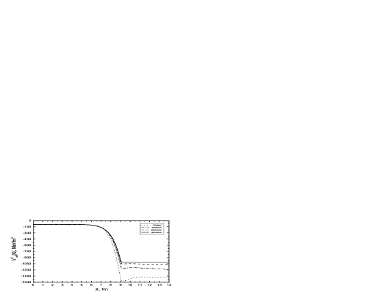
Figure 3: The Fermi averaged EPI ${\mathcal{V}}^{\mbox{\scriptsize F}}_{\mbox{\scriptsize eff}}(X)$ for different $E_{0}$.

It reveals a strong attraction outside the slab which changes rapidly in the surface region to rather weak attraction inside the slab. The asymptotic value of ${{\mathcal{V}}^{\mbox{\scriptsize F}}_{\mbox{\scriptsize eff}}}(X\to\infty)$ decreases with growing of $E_{0}$. As $E_{0}\to\infty$, the function ${{\mathcal{V}}^{\mbox{\scriptsize F}}_{\mbox{\scriptsize eff}}}(X)$ must tend to the analogous quantity ${\cal V}_{0}^{\mbox{\scriptsize F}}$ calculated for the free NN-interaction. The asymptotic value of ${\cal V}_{0}^{\mbox{\scriptsize F}}$ is ${\cal V}_{0}^{\mbox{\scriptsize F}}(X\to\infty){=}-720\;$MeV.

The situation with convergence of the integrals of Eq. (23) for the 2-particle propagator turned out to be more dramatic. A very slow convergence of this integral was noted in [13] where the problem of microscopic calculation of the EPI was analyzed, but the gap equation itself was not solved. Such a big value of the cutoff momentum as $K_{max}{=}60\;$fm^-1 was chosen to guarantee a reasonable accuracy of the EPI. The main reason of this phenomenon is the hard-core character of the Paris potential. Now we found that the gap $\Delta$ is much more sensitive to the cutoff than the EPI, and such a huge value as $K_{max}{=}160\div 180\;$fm^-1 is necessary to obtain $\Delta$ with 1% accuracy. It can be seen from Fig. 4 for the Fermi averaged gap $\Delta_{\mbox{\scriptsize F}}(X)$ calculated for different values of $K_{max}$. The corresponding results for the EPI are displayed in Fig. 5.

Figure 4: The Fermi averaged gap $\Delta_{\mbox{\scriptsize F}}(X)$ for different cut-off momenta $K_{max}$. The model space corresponds to $E_{0}=20$ MeV.

Figure 5: The Fermi averaged EPI ${\mathcal{V}}^{\mbox{\scriptsize F}}_{\mbox{\scriptsize eff}}(X)$ for different cut-off momenta $K_{max}$. The model space corresponds to $E_{0}=20$ MeV.

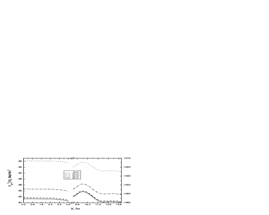
Figure 6: Details of Fig. 5 in an enlarged scale.

To emphasize the difference between the curves, we displayed in Fig. 6 the regions of small and large $X$ separately, in a enlarged scale. It is seen that the variation of the EPI with growing of $K_{max}$ from 60 fm^-1 to 180 fm^-1 looks quite small, but it leads to a noticeable enhancement of $\Delta_{\mbox{\scriptsize F}}(X)$. In fact, 1% variation of EPI results in 5%, or even more, change of $\Delta$. The reason of such a high sensitivity of $\Delta$ to a small variation of the EPI could be seen in the exponent dependence of $\Delta$ on the inverse effective interaction strength $1/g$ in the BCS formula (1). In this approximation, all depends on the value of $g$. Experience of solving the gap equation with Paris potential in infinite nuclear matter shows that in the region of the maximum of $\Delta$ ($k_{F}\simeq 0.8\;$fm^-1 ), where the effective $g$ is big, the convergence is not so slow. In this case, $K_{max}{=}20\;$fm^-1 is enough to reach 1% accuracy in $\Delta$. However, let us consider the density describing the inner region of the slab under consideration, $k_{F}{=}1.42\;$fm^-1, which corresponds to a small $\Delta$ (small $g$) situation. In this case, the convergence is very slow, and for 1% accuracy in $\Delta$ one needs in $K_{max}\simeq 200\;$fm^-1. Looking in Fig. 5, one could conclude that the surface region with a big EPI should dominate in the gap equation (27). In this case, the sensitivity of $\Delta$ to small variation of the EPI should not be so high. However, the comparison of Fig. 4 and Fig. 5 shows that the inner region with small EPI (and high sensitivity of $\Delta$ to $g$) should contribute to Eq. (27) significantly to explain this strong influence of a variation of $K_{max}$ on the value of $\Delta$.

To check this point, it is instructive to analyze the Fermi averaged anomalous density matrix $\kappa_{\mbox{\scriptsize F}}(X)$. It is displayed in Fig. 7 together with the EPI ${\mathcal{V}}^{\mbox{\scriptsize F}}_{\mbox{\scriptsize eff}}(X)$ and the product of ${\mathcal{V}}^{\mbox{\scriptsize F}}_{\mbox{\scriptsize eff}}(X)\,\kappa_{\mbox{\scriptsize F}}(X)$.

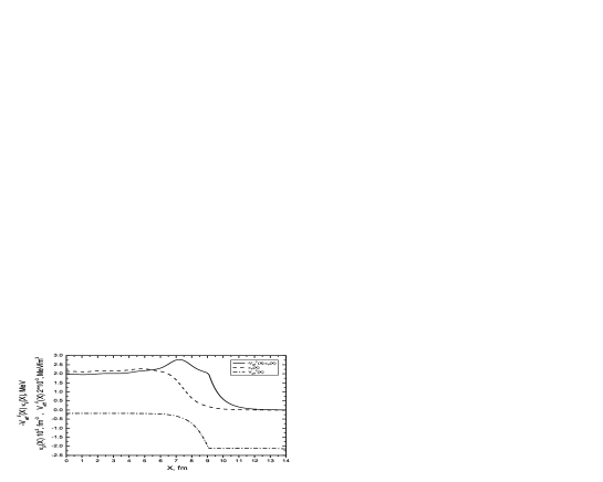
Figure 7: The Fermi averaged anomalous density $\kappa_{\mbox{\scriptsize F}}(X)$, EPI ${\mathcal{V}}^{\mbox{\scriptsize F}}_{\mbox{\scriptsize eff}}(X)$ and their product, in arbitrary units.

All the functions are drawn in arbitrary units, for the graphical convenience. It is seen that the anomalous density matrix falls rapidly down outside the slab. This decrease almost compensate the surface increase of the EPI in Eq. (27). Indeed, although the product function inside the slab is less than at the surface, the difference is not significant.

To examine a relevance of our previous approximate calculations of $\Delta$, it is worth to consider the so-called gap-shape function which was found in [1] with the help of a generalization of the KKC method [5] to non-homogeneous systems. It was defined as follows:

$$\chi(x_{1},x_{2};k^{2}_{\perp})=\Delta(x_{1},x_{2};k^{2}_{\perp})/\Delta_{\mbox{\scriptsize F}}(0).$$ (40)

Obviously, it can be represented as the sum

$$\chi(x_{1},x_{2};k^{2}_{\perp})=\sum\limits_{i}\chi_{i}(X)\,g_{i}(k^{2}_{\perp},x),$$ (41)

with components

$$\chi_{i}(X)=\Delta_{i}(X)/\Delta_{\mbox{\scriptsize F}}(0).$$ (42)

Let us again introduce the Fermi averaged gap-shape function

$$\chi_{\mbox{\scriptsize F}}(X)=\sum_{i}\chi_{i}(X)g_{i}(k^{2}_{\mbox{\scriptsize F}}(X)).$$ (43)

This quantity is displayed in Fig. 8 and Fig. 9 at different $E_{0}$ and $K_{max}$, correspondingly.

Figure 8: The Fermi averaged gap-shape function $\chi_{\mbox{\scriptsize F}}(X)$ for different $E_{0}$.

Figure 9: The Fermi averaged gap-shape function $\chi_{\mbox{\scriptsize F}}(X)$ for different $K_{max}$.

One can see that the gap-shape function is much less sensitive to a variation of these parameters than the gap itself. In fact, all the sensitivity of the gap is related to the normalization factor of $\Delta_{\mbox{\scriptsize F}}(0)$. Thus, our previous calculations of the gap-shape function with the use of $K_{max}{=}60\;$fm^-1 have sufficiently good accuracy. Such high sensitivity of the gap value to tiny variations of the calculation details shows a strong surface-volume interplay. In other words, it implies a significant proximity effect.

The results of the solution of the gap equation for $L{=}8\;$fm are presented in Fig. 10 (the separate components $\Delta_{i}(X)$) and in the Table 1 for the diagonal matrix elements $\Delta_{nn}(k_{\perp}{=}0)$, $n$ corresponding to the states with the positive parity.

Figure 10: The components of the gap $\Delta_{i}(X)$.

These are the matrix elements which could be related to those in heavy nuclei over the single-particle $s$-states. The typical value of the matrix elements $\Delta_{nn}$ is of the order of 1 MeV. The only exception is the one corresponding to very small energy $\varepsilon_{n}{=}-1.09\;$MeV. The reason is quite trivial. Indeed, the wave function has very long “tail” outside the slab, therefore the weight of $y_{n}(x)^{2}$ in the integral of $\Delta_{nn}$ is rather small in the region where the components $\Delta_{i}(X)$ are large. The average value of the gap in Table 1 is $\bar{\Delta}{=}0.85\;$MeV (and ${=}1.00\;$MeV, if to exclude the state with the small energy). The self-consistent value of the chemical potential $\mu{=}-7.96\;$MeV is very close to the one, $\mu_{0}{=}-8\;$MeV, without pairing. The difference $\delta\mu{=}-0.04\;$MeV is in agreement with the standard estimate $\delta\mu\sim-\Delta^{2}/\varepsilon_{\mbox{\scriptsize F}}$.

Table 1. Diagonal matrix elements $\Delta_{nn}(k_{{}_{\perp}}{=}0)$ in the slab with the width parameter $L{=}8\;$fm.

$\varepsilon_{n},\;$MeV	$\Delta_{nn},\;$MeV
-49.06	1.14
-42.16	1.11
-30.22	0.98
-15.22	0.76
-1.09	0.26

Let us now examine dependence of the results on the value of the width parameter $L$. The Fermi averaged gap functions for different $L$ are displayed in Fig. 11.

Figure 11: The Fermi averaged gap $\Delta_{\mbox{\scriptsize F}}(X)$ for different $L$.

The values of $L{=}6.2\;$fm and $L{=}7.4\;$fm are chosen to imitate nuclei of the tin and lead regions, correspondingly. The average diagonal matrix elements of $\Delta(k_{\perp}{=}0)$ are $\bar{\Delta}{=}1.08\;$MeV for Pb and $\bar{\Delta}{=}1.06\;$MeV for Sn. In the latter case, again there is a small energy level with a small value of $\Delta_{nn}$. If it will be excluded from the analysis, one obtains $\bar{\Delta}{=}1.26\;$MeV. In any case, these values are rather close to those in atomic nuclei which are about 1 MeV for the Pb isotopes and about 1.4 MeV, for Sn isotopes. As it is seen in Fig. 11, with increase of $L$ the surface maximum of the function $\Delta_{\mbox{\scriptsize F}}(X)$ becomes lower. At the same time, the central value $\Delta_{\mbox{\scriptsize F}}(X{=}0)$ becomes smaller. The corresponding values are given in Table 2. At the same time, the ratio $\alpha{}=\Delta_{\mbox{\scriptsize F}}^{max}/\Delta_{\mbox{\scriptsize F}}(0)$ depends on $L$ very smoothly.

Table 2. Dependence of the cental values $\Delta_{\mbox{\scriptsize F}}(X{=}0)$ on the width parameter $L$.

$L$, fm	$\Delta_{\mbox{\scriptsize F}}(X{=}0)\;$,MeV	$\Delta_{\mbox{\scriptsize F}}^{max}\;$,MeV	$\alpha$
6.2	0.45	1.20	2.67
7.4	0.46	1.09	2.37
8.0	0.41	0.94	2.29
14.0	0.36	0.88	2.44
20.0	0.30	0.77	2.57
$\infty$	0.22	-	-

The Fermi averaged gap-shape functions at different $L$ are displayed in Fig. 12. In agreement with Table 2, the values of the surface maximum are almost $L$-independent. Fig. 12 is in a good agreement with the analogous one in [1] obtained with the help of the KKC method.

Figure 12: The Fermi averaged gap-shape function $\chi_{\mbox{\scriptsize F}}(X)$ for different $L$.

4 Conclusions

We solved the gap equation in the ${}^{1}S_{0}$-channel for a nuclear slab with the separable $3\times 3$ representation [2, 3] of the Paris potential. A two-step method was used in which the gap equation is solved in the model space in terms of the EPI which is found in the complementary subspace. The model space is chosen sufficiently wide to make it possible to neglect the pairing effects in the complementary subspace. In this case, the EPI obeys the Bethe-Goldstone-type equation which was solved with the help of the so-called local-potential approximation which, as it was shown in [1], has very high accuracy. The absolute value of the gap $\Delta$ turned out to be very sensitive to the cutoff $K_{max}$ in the momentum space in the equation for the EPI. It is necessary to take $K_{max}{=}160\div 180\;$fm^-1 to guarantee 1% accuracy for $\Delta$.

The gap equation itself is solved directly, without any additional approximations. The solution shows the surface enhancement of the gap $\Delta$ which was earlier found [14] with an approximate consideration of the gap equation. A significant surface-volume interplay was observed also, thereby a kind of the proximity effect was found. The diagonal matrix elements of $\Delta$ which could be corresponded to those in heavy atomic nuclei turned out to be rather close to empirical values. Of course, there are various corrections to the BCS approximation. In nuclear matter, they came mainly from the screening of the EPI due to particle-hole excitations [15–18] and the dispersive self-energy effects [19]. In the nuclear slab system under consideration, just as in real atomic nuclei, they are partially suppressed due to the enhanced contribution of the surface region. Evidently, the most important correction to the BCS approximation is the one due to the surface vibrations [6]. In our calculations, the room for all the additional corrections to the BCS approximation is of order of 20%. This contradicts to some extent to results of Ref. [20, 21, 6] where the microscopic gap equation was solved directly for the spherical nucleus ¹²⁰Sn with Argonne NN-force $v14$, and only about 50% of the empirical value of $\Delta$ was obtained. The additional 50% was explained in [6] with the surface vibration contributions. We suppose that the main reason in the difference of our results of solving the BCS gap equation and those of Ref. [6] is in value of the effective nucleon mass $m^{*}$ which was chosen in [6] as the density dependent one varying from $m^{*}{=}0.7m$ inside the nucleus to $m^{*}{=}m$ outside. We used the value of $m^{*}{=}m$ which is, in our opinion, closer to the empirical effective mass in atomic nuclei. As to the surface vibration contribution itself, possibly, it is partially overestimated in [6] due to neglecting the so-called non-pole diagrams. This point is discussed in more detail in [1]. The problem of the consistent account of the non-pole diagrams in the pairing problem, along the line of [9], is waiting for its solution.

5 Acknowlegements

The authors are highly thankful to S.T. Belyaev and S.V. Tolokonnikov for helpful discussions. This research was partially supported by the Grant NS-1885.2003.2 of The Russian Ministry for Science and Education.

References

- [1] M. Baldo, U. Lombardo, E. E. Saperstein, M. V. Zverev, Phys. Rep. 391 261 (2004).
- [2] J. Haidenbauer, W. Plessas, Phys. Rev. C 30 (1984) 1822.
- [3] J. Haidenbauer, W. Plessas, Phys. Rev. C 32 (1985) 1424.
- [4] M. Lacombe, B. Loiseaux, J. M. Richard, R. Vinh Mau, J. Côté, D. Pirès and R. de Tourreil, Phys. Rev. C 21 (1980) 861.
- [5] V. A. Khodel, V. V. Khodel and J. W. Clark, Nucl. Phys. A 598 (1996) 390.
- [6] F. Barranco, R. A. Broglia, G. Colo, G. Gori, E. Vigezzi, and P. F. Bortignon. Eur. Phys. J. A 21 57 (2004).
- [7] M. Baldo, J. Cugnon, A. Lejeune, U. Lombardo, Nucl. Phys. A 515 (1990) 409.
- [8] E. Chabanat, P. Bonche, P. Haensel, J. Meyer, and R. Schaeffer, Nucl. Phys. A 627 (1997) 710.
- [9] V. A. Khodel and E. E. Saperstein, Phys. Rep. 92 (1982) 183.
- [10] G. E. Brown, J. H. Gunn and P. Gould, Nucl. Phys. 46 (1963) 598.
- [11] A. B. Migdal, Theory of finite Fermi systems and applications to atomic nuclei (Wiley, New York, 1967).
- [12] P. Ring, P. Schuck, The nuclear many-body problem (Springer, Berlin, 1980).
- [13] M. Baldo, U. Lombardo, E. E. Saperstein and M. V. Zverev, Nucl. Phys. A 628 (1998) 503.
- [14] M. Baldo, M. Farine, U. Lombardo, E. E. Saperstein, P. Schuck and M. V. Zverev, Eur. Phys. J. A 18 (2003) 17.
- [15] A. Schwenk, B. Friman and G. E. Brown, Nucl. Phys. A 703 (2002) 745.
- [16] T. L. Ainsworth, J. Wambach, and D. Pines, Phys. Lett. B 222 (1989) 173.
- [17] J. Wambach, T. L. Ainsworth, and D. Pines, Nucl. Phys. A 555 (1993) 128.
- [18] H.-J. Schulze, J. Cugnon, A. Lejeune, M. Baldo and U. Lombardo, Phys. Lett. B 375 (1996) 1.
- [19] M. Baldo and A. Grasso, Phys. Lett. B 485 (2000) 115.
- [20] S. G. Kadmensky, and P. A. Luk’yanovich, Sov. J. Nucl. Phys. 49 (1989) 238.
- [21] A. V. Avdeenkov, S. P. Kamerdzhiev, JETP Lett. 69 (1999) 715.