Pairing correlations in nuclei on the neutron-drip line

Abstract

Paring correlations in weakly bound nuclei on the edge of neutron drip line is studied by using a three-body model. A density-dependent contact interaction is employed to calculate the ground state of halo nuclei ⁶He and ¹¹Li, as well as a skin nucleus ²⁴O. Dipole excitations in these nuclei are also studied within the same model. We point out that the di-neutron type correlation plays a dominant role in the halo nuclei ⁶He and ¹¹Li having the coupled spin of the two neutrons $S$=0, while the correlation similar to the BCS type is important in ²⁴O. Contributions of the spin $S$=1 and S=0 configurations are separately discussed in the low energy dipole excitations.

I Introduction

It is now feasible to study the structure of nuclei on the edge of neutron drip line. Such nuclei are expected to have unique properties influenced by the large spatial distribution of weakly bound valence neutrons, for examples, halo, skin, new magic numbers and strong soft dipole excitations.

Two-neutron halo nuclei (sometimes referred to as borromean nuclei when there is no bound state between a valence neutron and a core nucleus) like ⁶He and ¹¹Li have been often described as three-body systems consisting of two valence neutrons interacting with each other, and with the core BF1 ; BF2 ; BF3 ; VMP96 ; BVM97 ; Zhukov93 ; Fed95 . The three-body Hamiltonian with realistic two-body interactions has been solved by the Faddeev method Zhukov93 ; Fed95 . On the other hand, Bertsch and Esbensen have developed a three-body model with a density-dependent delta interaction among the valence neutrons BF1 . They have subsequently extended their model by taking into account the effect of the recoil of the core nucleusBF3 . They showed that the density-dependent contact force well reproduces the results of Faddeev calculations even though the radial dependence of the adopted interactions are quite different BF3 . To the date, the most sophisticated many-body calculations of light nuclei include also three-body forces which play an important role in obtaining the correct binding energies of light nuclei Pud95 . To a large extent, such three-body forces can also be simulated effectively by a density dependent force.

Recently, a Hartree-Fock-Bogoliubov (HFB) model has been applied to study a di-neutron structure of the drip line nuclei. The dipole response has also been studied with the quasi-particle random phase approximation (QRPA) taking into account the continuum effect Matsuo . Cluster models have also been often used to study the borromean nuclei including the dipole excitations Aoyama ; Myo .

In this paper, we undertake a detailed discussion on the ground state as well as the dipole response of neutron-rich nuclei using a three-body model with the density-dependent delta force, paying special attention to the di-neutron structure of valence neutrons. We particularly study the borromean nuclei, ⁶He and ¹¹Li, and also another drip line nucleus ²⁴O as a comparison. Since ²³O is bound, ²⁴O is not a borromean nucleus by definition, although the root-mean-square (rms) radius indicates a feature of very extended neutron wave functions. The model we use is essentially the same as that of Bertsch and EsbensenBF1 ; BF2 ; BF3 , while the interaction is adjusted to fit the separation energy of each drip line nucleus.

The paper is organized as follows. In Sec. II, we discuss the three-body model and the adopted two-body interactions. The results for the borromean nuclei are compared with those for the drip line nucleus ²⁴O in Sec. III. A summary is given in Sec. IV.

II Three-body model

We consider a three-body system consisting of two valence neutrons, and an inert core nucleus with the mass number $A_{c}$. We use the same three-body Hamiltonian as in Ref. BF3 . That is,

$$H=\hat{h}_{nC}(1)+\hat{h}_{nC}(2)+V_{nn}+\frac{\mbox{\boldmath$p$}_{1}\cdot\mbox{\boldmath$p$}_{2}}{A_{c}m}.$$ (1)

Here, $\hat{h}_{nC}$ is the single-particle Hamiltonian for a valence neutron interacting with the core and is given by

$$\hat{h}_{nC}=\frac{p^{2}}{2\mu}+V_{nC}(r),$$ (2)

where $\mu=mA_{c}/(A_{c}+1)$ is the reduced mass. The reduced mass $\mu$, together with the last term in Eq. (1), originate from the recoil kinetic energy of the coreBF3 . $V_{nn}$ is the interaction between the valence neutrons given by

$$V_{nn}(\mbox{\boldmath$r$}_{1},\mbox{\boldmath$r$}_{2})=\delta(\mbox{\boldmath$r$}_{1}-\mbox{\boldmath$r$}_{2})\left(v_{0}+\frac{v_{\rho}}{1+\exp[(r_{1}-R_{\rho})/a_{\rho}]}\right).$$ (3)

It is well known that the delta force (3) must be supplemented with an energy cutoff $E_{\rm cut}$ in the two-particle spectrum. In terms of the energy cutoff $E_{\rm cut}$ and the scattering length $a_{nn}$ for $nn$ scattering, the strength for the delta interaction $v_{0}$ is given by BF3

$$v_{0}=\frac{2\pi^{2}\hbar^{2}}{m}\,\frac{2a_{nn}}{\pi-2k_{c}\,a_{nn}},$$ (4)

where $E_{\rm cut}=\hbar^{2}k_{c}^{2}/m$. The parameters for the density dependent part, i.e., $v_{\rho},R_{\rho}$, and $a_{\rho}$, are adjusted in order to reproduce the known ground state properties for each nucleus. We specify the value of the parameters below.

We diagonalize the Hamiltonian (1) in the model space of the two-particle states with the energy $\epsilon_{1}+\epsilon_{2}\leq(A_{c}+1)E_{\rm cut}/A_{c}$ BF3 , where $\epsilon$ is a single-particle energy of valence particle. We use a Woods-Saxon potential for $V_{nC}$ to generate the single-particle basis:

$$V_{nC}(r) = V_{0}\left(1-0.44f_{so}r_{0}^{2}(\mbox{\boldmath$l$}\cdot\mbox{\boldmath$s$})\frac{1}{r}\frac{d}{dr}\right)$$ (5)

$$~{}~{}~{}\times\left[1+\exp\left(\frac{r-R}{a}\right)\right]^{-1},$$

where $R=r_{0}A_{c}^{1/3}$. For ⁶He, we use the parameter set $a$=0.65 fm, $r_{0}$=1.25 fm, $V_{0}=-47.4$ MeV, and $f_{so}$=0.93, that reproduces the measured low-energy $n$-$\alpha$ phase shifts BF3 . We employ the same parameters for the density-dependent interaction as in the line 5 of Table II in Ref. BF3 : $a_{nn}=-15$ fm, $E_{\rm cut}=40$ MeV, $v_{\rho}=-v_{0}$, $R_{\rho}$=2.436 fm, and $a_{\rho}$=0.67 fm. The continuum single-particle spectrum is discretized with a radial box of $R_{\rm box}=30$ fm.

For ¹¹Li, we use $a$=0.67 fm, $r_{0}$=1.27 fm, $f_{so}$=1.006, and $R_{\rm box}=40$ fm. For the Woods-Saxon potential, a deep potential $V_{0}=-47.5$ MeV is used for the even parity states, while a shallow potential $V_{0}=-35.366$ MeV is adopted for the odd parity states in order to increase the $s$-wave component of the ground state wave function BF3 . Similar potentials are used also in Ref. VMP96 . For the density dependent force, we use a similar parameter set $a_{nn}=-15$ fm, $E_{\rm cut}=30$ MeV, $v_{\rho}=-v_{0}$, $R_{\rho}$=2.935 fm, and $a_{\rho}$=0.67 fm to that of the line 5 in Table IV in Ref. BF3 except the value of the energy cutoff.

For ²⁴O, we use $V_{0}=-43.2$ MeV, $a$=0.67 fm, $r_{0}$=1.25 fm, $f_{so}$=0.73, and $R_{\rm box}=30$ fm so that the bound s_1/2 and d_5/2 states have empirical single-particle energies $-2.739$ and $-3.806$ MeV observed in ²³O and ²¹O, respectively. For the pairing interaction, we use $a_{nn}=-15$ fm, $E_{\rm cut}=30$ MeV, $v_{\rho}=814.2$ MeV fm³, $R_{\rho}=R$, and $a_{\rho}$=0.67 fm which reproduce the two neutron separation energy of ²⁴O, S_2n=6.452 MeV.

The calculated ground state properties are summarized in Table 1, where

$$\langle r_{nn}^{2}\rangle=\langle\Psi_{gs}|(\mbox{\boldmath$r$}_{1}-\mbox{\boldmath$r$}_{2})^{2}|\Psi_{gs}\rangle,$$ (6)

is the mean square distance between the valence neutrons, and

$$\langle r_{c-2n}^{2}\rangle=\langle\Psi_{gs}|(\mbox{\boldmath$r$}_{1}+\mbox{\boldmath$r$}_{2})^{2}/4|\Psi_{gs}\rangle,$$ (7)

is the mean square distance of their center of mass with respect to the core.

Table 1: Ground state properties of ⁶He, ¹¹Li, and ²⁴O obtained with the three-body model with the density-dependent delta interaction. The result for ⁶He is the same as the line 5 in Table II in Ref. BF3 .

nucleus	$S_{2n}$	$\langle r_{nn}^{2}\rangle$	$\langle r_{c-2n}^{2}\rangle$	dominant	fraction
	(MeV)	(fm2)	(fm2)	configuration	(%)
6He	0.975	21.3	13.2	(p${}_{3/2})^{2}$	83.0
11Li	0.295	41.4	26.3	(p${}_{1/2})^{2}$	59.1
24O	6.452	35.2	10.97	(s${}_{1/2})^{2}$	93.6

III Discussions

III.1 Ground state properties

Let us now discuss the spatial correlation of the valence neutrons in the ground state, and its influence to the dipole excitations near the neutron threshold. To this end, we first plot the two-particle density. It is given as a function of two radial coordinates, $r_{1}$ and $r_{2}$, for the valence neutrons, and the angle between them, $\theta_{12}$. The two-particle density can be decomposed into the $S=0$ and $S=1$ components in the $LS$-coupling scheme, i.e.,

$$\rho_{2}(r_{1},r_{2},\theta_{12})=\rho^{S=0}_{2}(r_{1},r_{2},\theta_{12})+\rho^{S=1}_{2}(r_{1},r_{2},\theta_{12}).$$ (8)

The explicit expression for the each component is given by BF1

$$\rho^{S=0}_{2}(r_{1},r_{2},\theta_{12})=$$

$$\frac{1}{8\pi}\sum_{L}\sum_{l,j}\sum_{l^{\prime},j^{\prime}}\frac{\hat{l}\hat{l^{\prime}}\hat{L}}{\sqrt{4\pi}}\left(\begin{array}[]{ccc}l&l^{\prime}&L\\ 0&0&0\end{array}\right)^{2}$$ (11)

$$~{}\times\Phi_{lj}(r_{1},r_{2})\Phi_{l^{\prime}j^{\prime}}(r_{1},r_{2})Y_{L0}(\theta_{12})$$

$$~{}\times(-)^{l+l^{\prime}}\sqrt{\frac{2j+1}{2l+1}}\sqrt{\frac{2j^{\prime}+1}{2l^{\prime}+1}},$$ (12)

$$\rho^{S=1}_{2}(r_{1},r_{2},\theta_{12})=$$

$$\frac{1}{8\pi}\sum_{L}\sum_{l,j}\sum_{l^{\prime},j^{\prime}}\frac{\hat{l}\hat{l^{\prime}}\hat{L}}{\sqrt{4\pi}}\left(\begin{array}[]{ccc}l&l^{\prime}&L\\ 0&0&0\end{array}\right)\left(\begin{array}[]{ccc}l&l^{\prime}&L\\ 1&-1&0\end{array}\right)$$ (17)

$$~{}\times\Phi_{lj}(r_{1},r_{2})\Phi_{l^{\prime}j^{\prime}}(r_{1},r_{2})Y_{L0}(\theta_{12})$$

$$~{}\times(-)^{j+j^{\prime}}\sqrt{2-\frac{2j+1}{2l+1}}\sqrt{2-\frac{2j^{\prime}+1}{2l^{\prime}+1}},$$ (18)

where $\hat{l}=\sqrt{2l+1}$. Here, $\Phi_{lj}(r,r^{\prime})$ is the radial part of the two-particle wave function defined as

$$\Phi_{lj}(r,r^{\prime}) = \sum_{n^{\prime}\leq n}\frac{\alpha_{nn^{\prime}lj}}{\sqrt{2(1+\delta_{n,n^{\prime}})}}$$ (19)

$$\times (\phi_{nlj}(r)\phi_{n^{\prime}lj}(r^{\prime})+\phi_{nlj}(r^{\prime})\phi_{n^{\prime}lj}(r)),$$

where $n$ and $n^{\prime}$ are the radial quantum numbers and $\alpha_{nn^{\prime}lj}$ is the expansion coefficient. $\phi_{nlj}(r)$ is the radial part of the Woods-Saxon single particle wave function. Notice that the two-particle density is normalized as

$$\int_{0}^{\infty}4\pi r_{1}^{2}\,dr_{1}\int_{0}^{\infty}r_{2}^{2}\,dr_{2}\int_{0}^{\pi}2\pi\sin\theta_{12}\,d\theta_{12}\,\rho_{2}(r_{1},r_{2},\theta_{12})=1.$$ (20)

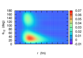
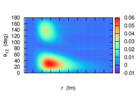
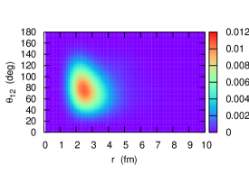
Figure 1: (Color online) The two-particle density for ⁶He as a function of $r_{1}=r_{2}=r$ and the angle between the valence neutrons, $\theta_{12}$. The two-particle density is weighted with a factor $4\pi r^{2}\cdot 2\pi r^{2}\sin\theta_{12}$. The top panel shows the total density, while the middle and the bottom panels show the $S$=0 and the $S$=1 components in the $LS$-coupling scheme, respectively.

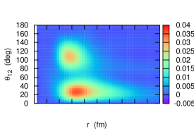
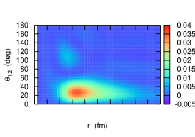
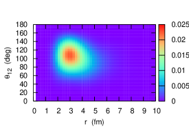
Figure 2: (Color online) Same as fig. 1, but for ¹¹Li.

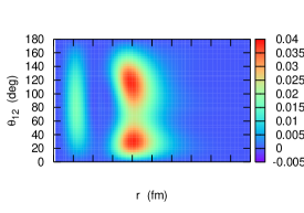
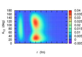
Figure 3: (Color online) Same as fig. 1, but for ²⁴O.

Figures 1,2, and 3 show the (total) two-particle density (the top panels) for the ⁶He, ¹¹Li, and ²⁴O nuclei, respectively, and their spin decompositions (the middle and the bottom panels). These are plotted as a function of the radius $r_{1}=r_{2}\equiv r$ and the angle $\theta_{12}$, and with a weight of $4\pi r^{2}\cdot 2\pi r^{2}\sin\theta_{12}$. As has been pointed out in Refs. BF1 ; Zhukov93 ; OZV99 , one observes two peaks in the two-particle densities, although the two peaked structure is somewhat smeared in ²⁴O. The peaks at smaller and larger $\theta_{12}$ are referred to as “di-neutron” and “cigar-like” configurations in Refs. Zhukov93 ; OZV99 , respectively. We see that the di-neutron part of the two-particle density has a long radial tail in ⁶He and ¹¹Li, and thus can be interpreted as a halo structure. In contrast, the cigar-like configuration has a rather compact radial shape. For ²⁴O, the di-neutron and the cigar-like configurations behave similarly as a function of $r$, and do not show a halo structure. Evidently, a large rms radius of ²⁴O is attributed to the dominant $s$-wave component in the ground state wave function, rather than the halo effect (see below).

We find that the spin structure of the two-particle density is considerably different among the three nuclei studied. In order to see this transparently, we introduce the angular density $\rho(\theta_{12})$ by integrating the radial coordinates in the two-particle density, i.e.,

$$\rho(\theta_{12})\equiv 4\pi\int_{0}^{\infty}r_{1}^{2}\,dr_{1}\int_{0}^{\infty}r_{2}^{2}\,dr_{2}\rho_{2}(r_{1},r_{2},\theta_{12}).$$ (21)

The angular density is normalized to unity as

$$2\pi\int_{0}^{\pi}\sin\theta_{12}\,d\theta_{12}\,\rho(\theta_{12})=1.$$ (22)

Fig. 4 shows the angular density for the ⁶He, ¹¹Li, and ²⁴O (with a weight of $2\pi\sin\theta_{12}$). The solid line is the total density, while the dashed and the dotted lines are for the $S=0$ and the $S=1$ components, respectively. The expectation value of the angle $\theta_{12}$ is 66.33, 65.29, and 82.37 degree. for ⁶He, ¹¹Li, and ²⁴O, respectively. For the borromean nuclei ⁶He and ¹¹Li, the $S$=0 wave function dominates the di-neutron part of the two-particle density. In contrast, the cigar-like part has a large $S$=1 part in ¹¹Li, but still the $S$=0 component dominates in ⁶He. For the ²⁴O nucleus, there is no clear separation between the di-neutron and the cigar-like type structures. The wave function shows a strong correlation typical in the BCS type wave function. In fact, the calculated rms radius for ²⁴O, 4.45 fm, is close to that of the bound 2s_1/2 state, 4.65 fm. A small difference in the rms radii is due to the anti-halo effect, caused by the pairing correlation BDP00 .

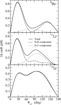
Figure 4: The angular density defined by Eq. (21) (weighted with a factor $2\pi\sin\theta$) for ⁶He, ¹¹Li, and ²⁴O. The solid line is for the total density, while the dashed and the dotted lines are for the $S$=0 and the $S$=1 components in the $LS$-coupling scheme, respectively.

The main features of the angular dependence of the two-particle density shown in Fig. 4 can be understood in the following way. From Eqs. (12) and (18), one can obtain by inserting the values of 3$j$-symbols that

$$\rho^{S=0}(\theta_{12}) \propto \frac{1}{3}Y_{00}(\theta_{12})+\frac{2\sqrt{5}}{15}Y_{20}(\theta_{12})\propto\cos^{2}\theta_{12}$$ (23)

$$\rho^{S=1}(\theta_{12}) \propto \frac{1}{3}Y_{00}(\theta_{12})-\frac{5}{\sqrt{15}}Y_{20}(\theta_{12})\propto\sin^{2}\theta_{12}$$ (24)

for the configurations $(j,l)=(j^{\prime},l^{\prime})=$p_3/2 or $(j,l)=(j^{\prime},l^{\prime})=$p_1/2 . When weighted by $\sin\theta_{12}$, Eq. (23) has a peak at $\theta_{12}$=35.26 degree and 144.74 degree, while Eq. (24) has the maximum at $\theta_{12}$=90 degree. This is indeed the case for the ⁶He nucleus. For the ¹¹Li, the admixture of the (s${}_{1/2})^{2}$ and (d${}_{5/2})^{2}$ configurations perturb this picture, and a peak at $\theta_{12}$=144.74 degree in the $S$=0 component disappears to a large extent. For the ²⁴O nucleus, the $S=1$ component is largely suppressed since the pure (s${}_{1/2})^{2}$ state cannot form the $S=1$ configuration. Also, the two-particle density for the pure (s${}_{1/2})^{2}$ configuration is proportional to $|Y_{00}|^{2}$, and thus has a peak at $\theta_{12}$=90 degree when it is weighted by $\sin\theta_{12}$.

III.2 Dipole excitations

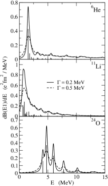
Figure 5: The B(E1) distribution for ⁶He, ¹¹Li, and ²⁴O. The solid and the dashed lines are obtained with a smearing procedure with $\Gamma=0.2$ and 0.5 MeV, respectively.

We next discuss the response of the ground state to the dipole field,

$$\hat{D}_{M}=-\frac{Z}{A}e\,(r_{1}Y_{1M}(\hat{\mbox{\boldmath$r$}}_{1})+r_{2}Y_{1M}(\hat{\mbox{\boldmath$r$}}_{2})).$$ (25)

Since we obtain the excited 1^- states by the matrix diagonalization, they appear as discrete states. We smear the discrete strength distribution with a smearing function as

$$B(E1)=\sum_{k}\,\frac{\Gamma}{\pi}\,\frac{1}{(E-E_{k})^{2}+\Gamma^{2}}\,B_{k}(E1),$$ (26)

where $B_{k}(E1)$ is the $B(E1)$ strength for the $k$-th excited state,

$$B_{k}(E1)=3\,|\langle\Psi_{1^{-}}^{k}|\hat{D}_{0}|\Psi_{gs}\rangle|^{2}.$$ (27)

Fig. 5 shows the $B(E1)$ distributions for the ⁶He, ¹¹Li, and ²⁴O. The solid and the dashed lines are obtained with the smearing function (26) with $\Gamma$=0.2 and 0.5 MeV, respectively. The discrete distributions are also shown. The total $B(E1)$ strength, $\sum_{k}B_{k}(E1)$, is 1.31, 1.76 and 0.97 $e^{2}$ fm² for the ⁶He, ¹¹Li, and ²⁴O, respectively.

We notice that the strong threshold peak appears in the response of ⁶He and ¹¹Li. In the cluster model within the plane wave approximation, the peak of the strength function appears at 1.6$S_{c}$, where $S_{c}$ is the cluster separation energy STG92 ; BBH91 ; HHB03 . The calculated peaks in Fig. 5 are at 1.55 and 0.66 MeV for ⁶He and ¹¹Li, respectively. These peaks are very close to 1.6 times the two neutron separation energy, 1.6$S_{2n}$=1.56 MeV for ⁶He and 0.47 MeV for ¹¹Li. This similarity suggests the existence of strong di-neutron correlations in these nuclei. A small difference between the peak energy in Fig. 5 and 1.6$S_{2n}$ for ¹¹Li is due to the large configuration mixing of s_1/2 state (22.7%) in the ground state. In contrast, for ²⁴O, the peak (4.78 MeV) is below the two neutron separation energy, and is rather close to 1.6 times single particle energy for the 2s_1/2 state, that is, 1.6$\times$ 2.74 = 4.38 MeV. Therefore, the di-neutron correlation does not seem to play a major role in the dipole response in this nucleus.

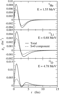
Figure 6: The transition density for the state close to the peak in the the B(E1) distribution. The top, middle, and bottom panels are for ⁶He, ¹¹Li, and ²⁴O, respectively. The solid line indicates the total density, while the $S$=0 component is denoted by the dashed line.

In order to see the threshold effect more clearly, we plot in Fig. 6 the transition density for the strong E1 peaks for each nucleus. As a comparison, we also show the $S$=0 component of the transition density by the dashed line. For ⁶He and ¹¹Li, the transition density shows a nodal structure and changes its sign, that is typical in the coupling to the continuum spectrum. Also, the $S$=0 component plays a significant role, supporting the importance of the di-neutron correlation in these nuclei. On the other hand, such clear nodal structure is not seen in the transition density of ²⁴O. The transition density seems to consist of a coherent sum of the $S$=0 and the $S$=1 components. The dipole excitation in ²⁴O is therefore interpreted as a coherent superposition of particle-hole excitations, rather than the continuum excitations, as in stable nuclei where the continuum effect is much less important.

We mention that, while the Coulomb breakup for the one-neutron halo ¹¹Be is now well established, that for the two-neutron halo ¹¹Li is still in dispute showing large discrepancies between the experimental data taken by three different groups Li11_exp . Recently, Nakamura and his collaborators performed the Coulomb dissociation experiments of ¹¹Li on ²⁰⁸Pb target with much higher statistics and with much less ambiguities caused by cross talk events in detecting two neutrons NF05 . They observed a sharp peak at E${}_{\rm exp}\sim$0.6MeV and the integrated strength B_exp(E1)=1.5$\pm 0.1e^{2}$ fm² for E$<$ 3.3MeV, which are consistent with the present results E_peak=0.66 MeV with the calculated strength B_cal(E1)=1.31 $e^{2}$ fm² for E$<$ 3.3MeV. Similar calculated results were also reported in Ref. BF3 .

IV SUMMARY

We have studied the role of di-neutron correlations in weakly bound nuclei on the neutron drip line using a three-body model. The model Hamiltonian consists of a Woods-Saxon potential between a valence neutron and the core, and of a density-dependent pairing interaction among the valence neutrons. We applied this model to the borromean nuclei, ⁶He and ¹¹Li, as well as a skin nucleus ²⁴O. For the borromean nuclei, ⁶He and ¹¹Li, we found that the two-particle density has a two peaked structure, one peak at a small opening angle between the valence neutrons and the other at a large angle (the ’di-neutron’ and ’cigar-like’ configurations, respectively). We found that the former is dominated by the $S$=0 configurations in the $LS$ coupling scheme and has a long tail. On the other hand, the latter has a compact shape, and is dominated by the $S$=1 configuration for ¹¹Li while by the $S$=0 configuration for ⁶He. For ²⁴O, there is no clear separation between the di-neutron and the cigar-like configurations, and the ground state is dominated by the $S$=0 configuration.

We have also studied the dipole response of these nuclei within the same model. We found strong threshold peaks in the response of ⁶He and ¹¹Li nuclei, where the transition density shows the importance of the coupling to the continuum. The $S$=0 configuration, thus the di-neutron correlation, was found to have a large contribution to the transition density for these peaks. On the other hand, no clear sign of the continuum coupling was seen in the response of ²⁴O. The transition density for the low energy dipole strength of ²⁴O consists of a coherent sum of the $S$=0 and the $S$=1 components, and therefore the di-neutron correlation plays a much less important role in ²⁴O than in the borromean nuclei.

Recently, a new Coulomb breakup measurement for ¹¹Li has been undertaken at RIKEN NF05 . It would be interesting to perform a similar experiment also for the ²⁴O nucleus and see a difference between them as we discussed in this paper.

- (1) G.F. Bertsch and H. Esbensen, Ann. Phys. (N.Y.) 209, 327 (1991).
- (2) H. Esbensen and G.F. Bertsch, Nucl. Phys. A542, 310 (1992).
- (3) H. Esbensen, G. F. Bertsch and K. Hencken, Phys. Rev. C56, 3054 (1999).
- (4) N. Vinh Mau and J.C. Pacheco, Nucl. Phys. A607, 163 (1996).
- (5) A. Bonaccorso and N. Vinh Mau, Nucl. Phys. A615, 245 (1997).
- (6) M.V. Zhukov et al., Phys. Rep. 231, 151 (1993).
- (7) D. V. Fedorov, E. Garrido and A. S. Jensen, Phys. Rev. C51, 3052 (1995).
- (8) B. S. Pudliner, V. R. Pandharipande, J. Carlson and R. B. Wiringa, Phys. Rev. Lett. 74, 4396 (1995); S. C. Pieper, V. R. Pandharipande, R. B. Wiringa and J. Carlson, Phys. Rev. C64, 014001 (2001).
- (9) M. Matsuo, K. Mizuyama and Y. Serizawa, Phys. Rev. C71, 064326 (2005).
- (10) S. Aoyama, K. Kato and K. Ikeda, Prog. Theor. Phys. Suppl. 142, 35 (2001); T. Myo, S. Aoyama, K. Kato and K. Ikeda, Prog. Theor. Phys. 108, 133 (2002).
- (11) T. Myo, S. Aoyama, K. Kato, and K. Ikeda, Phys. Lett. B576, 281 (2003); T. Myo, K. Kato, S. Aoyama, and K. Ikeda, Phys. Rev. C63, 054313 (2001).
- (12) Yu. Ts. Oganessian, V.I. Zagrebaev, and J.S. Vaagen, Phys. Rev. Lett. 82, 4996 (1999); Phys. Rev. C60, 044605 (1999).
- (13) K. Bennaceur, J. Dobaczewski, and M. Ploszajczak, Phys. Lett. B496, 154 (2000).
- (14) H. Sagawa, N. Takigawa, and Nguyen Van Giai, Nucl. Phys. A543, 575 (1992).
- (15) C.A. Bertulani, G. Baur, and M.S. Hussein, Nucl. Phys. A526, 751 (1991).
- (16) K. Hagino, M.S. Hussein, and A.B. Balantekin, Phys. Rev. C68, 048801 (2003).
- (17) K. Ieki et al., Phys. Rev. Lett. 70, 730 (1993); S. Shimoura et al., Phys. Lett. B348, 29 (1995); M. Zinser et al., Nucl. Phys. A619, 151 (1997).
- (18) T. Nakamura and N. Fukuda, Eur. Phys. J. A, in press (2005).