Dipole resonances in light neutron-rich nuclei studied with time-dependent calculations of antisymmetrized molecular dynamics

Abstract

In order to study isovector dipole response of neutron-rich nuclei, we have applied a time-dependent method of antisymmetrized molecular dynamics. The dipole resonances in Be, B and C isotopes have been investigated. In ¹⁰Be, ¹⁵B, ¹⁶C, collective modes of the vibration between a core and valence neutrons cause soft resonances at the excitation energy $E_{x}=10-15$ MeV below the giant dipole resonance(GDR). In ¹⁶C, we found that a remarkable peak at $E_{x}=14$ MeV corresponds to coherent motion of four valence neutrons against a ¹²C core, while the GDR arises from the core vibration in the $E_{x}>20$ MeV region. In ¹⁷B and ¹⁸C, the dipole strengths in the low energy region decline compared with those in ¹⁵B and ¹⁶C. We also discuss the energy weighted sum rule for the $E1$ transitions.

I Introduction

In neutron-rich nuclei, there often appear exotic phenomena which are very different from those in stable nuclei due to the excess neutrons. Some properties of neutron-rich nuclei are concerned with differences between proton and neutron densities. Neutron halo and skin structures are typical examples. Another related subject is deformations of proton and neutron densities. For example, the difference of the deformations between proton and neutron densities were theoretically suggested in some Be, B and C isotopes [1, 2, 3]. These phenomena imply that the structure of the nuclei far from the $\beta$-stability line often contradicts to the usual understanding for stable nuclei where the proton and neutron densities are consistent with each other in a nucleus. They may lead also to exotic phenomena in excitations and reactions. One of the current issues is the dipole excitations in neutron-rich nuclei [4, 5, 6, 7, 8, 9, 10, 11, 12, 13, 14, 15, 16, 17, 18, 19, 20, 21]. Since it is quite natural to expect the low-energy isovector-dipole excitations due to the difference between the proton and neutron densities, interests are attracted to the soft resonances below the giant dipole resonance(GDR), their collectivity and the contributions of the excess neutrons. In fact, the features of dipole transitions in neutron-rich O isotopes have been studied experimentally[20] and theoretically [11, 13, 16]. They have been found to be different from those in the stable nucleus, ¹⁶O, especially in the low energy region below the GDR. The dipole excitations have been studied also in C isotopes by Suzuki et al. with shell model calculations[17], where they suggested that coherent neutron transitions enhance the strengths at the excitation energy $E_{x}=10-15$ MeV.

Our present interest is in the isovector dipole excitations in the light neutron-rich nuclei and in the effect of the ground state properties like the deformations on the $E1$ strengths. A method of antisymmetrized molecular dynamics(AMD)[1] is one of powerful approaches for nuclear structure study. The method is superior especially in the description of cluster aspect, which is important in light unstable nuclei as well as in light stable nuclei[22]. In the systematic studies of Be, B, and C isotopes performed with the AMD method, a variety of structure such as the neutron skin and the deformed states have been suggested in those nuclei, and some of them have been discussed in relation to cluster aspect[1, 22]. The experimental data for various properties of the neutron-rich Be, B and C isotopes have been successfully reproduced by the AMD calculations. We should stress that the AMD calculations well agree to the experimental data of quadrupole moments and $E2$ strengths in neutron-rich B and C, which can not be reproduced by the shell model calculations without using system-dependent effective charges. For the study of dipole excitations in the AMD framework, we apply a time-dependent method and calculate the dipole strengths in a similar way to the the time-dependent Hartree-Fock(TDHF). The point is that we are able to study dipole resonances with the framework which can describe cluster aspect. One of the advantages of the time-dependent AMD is that we can link the excitations with such collective modes as core vibration, core-neutron motion and inter-cluster motion which should be important to understand the role of the excess neutrons in the dipole resonances.

The time-dependent method of AMD have been proposed and applied to heavy-ion reactions by Ono et al. in 1992[23, 24] earlier than the application of the AMD to the nuclear structure study. For collective motion on the static solution, however, the time-dependent AMD calculations have not been performed yet. In this paper, we formulate a method based of the time-dependent AMD for the study of $E1$ response in analogy to the TDHF. In order to see its validity, we first apply it to ¹²C and ¹⁸O, and show comparison with the experimental data and other theoretical calculations. Then we apply this method to Be, B and C isotopes and discuss the properties of dipole strengths in the neutron-rich nuclei. We try to see how the dipole strength distribution is influenced by such structure as deformations, neutron skin, the existence of core and clusters.

This paper is organized as follows. In the next section, we explain the formulation of the present method for the $E1$ response, which is based on the time-dependent AMD. Adopted effective nuclear forces are described in III. In IV, we show the results of ¹²C, ¹⁸O and the comparison with the experimental data, and also the dipole transitions in Be, B, C isotopes. The discussion of the $E1$ excitations in neutron-rich Be, B, and C isotopes are given in V. Finally, in VI we give a summary.

II Formulation

We explain the formulation of the time-dependent version of AMD for study of isovector dipole excitations. By simulating time evolution of the collective motion on the static solution with the time-dependent AMD, we can calculate the response of a nucleus to external dipole fields and obtain the dipole strengths in the similar way to TDHF approaches.

The time-dependent method in the AMD framework is described in Refs.[23, 24], where the method has been applied to heavy-ion collisions. Concerning nuclear structure study with AMD methods, the static version of AMD and its extended versions are reviewed in Refs. [22, 25].

A Wave function

The wave function for a $A$-nucleon system($A$ is a mass number) is given by a single Slater determinant of Gaussian wave packets as,

$$\Phi=\frac{1}{\sqrt{A!}}{\cal{A}}\{\varphi_{1},\varphi_{2},...,\varphi_{A}\},$$ (1)

where the $i$-th single-particle wave function is written as follows,

$$\varphi_{i} = \phi_{{\bf Z}_{i}}\chi_{i}\tau_{i},$$ (2)

$$\phi_{{\bf Z}_{i}}({\bf r}_{j}) = (\frac{2\nu}{\pi})^{3/4}\exp\bigl{\{}-\nu({\bf r}_{j}-\frac{{\bf Z}_{i}}{\sqrt{\nu}})^{2}\bigr{\}},$$ (3)

$$\chi_{i} = (\frac{1}{2}+\xi_{i})\chi_{\uparrow}+(\frac{1}{2}-\xi_{i})\chi_{\downarrow}.$$ (4)

Here, the spatial part of the $i$-the single particle wave function is given by a located Gaussian wave packet, whose center is represented by the complex parameter, ${\bf Z}_{i}$. The parameter $\xi_{i}$ indicates the orientation of the intrinsic spin, and the iso-spin function is up(proton) or down(neutron).

In the present work, the orientation of the intrinsic spin is fixed to be up or down as $\xi_{i}=\{1/2,-1/2\}$ for simplicity. In this AMD wave function, all the centers of Gaussian wave packets for $A$ nucleons are independent variational parameters, and a set of parameters ${\bf Z}\equiv\{{\bf Z}_{1}$, ${\bf Z}_{2}$, $\cdots$, ${\bf Z}_{A}\}$ specifies the total wave function $\Phi({\bf Z})$ of the state. This is the simplest version of AMD wave function, and the parity and angular momentum projections are not performed in the present work.

B Equation of motion

In the time-dependent version of AMD, components of ${\bf Z}$ are considered to be time-dependent parameters as explained in [24]. The time evolution of the system is determined by the time-dependent variational principle,

$$\delta\int^{t_{2}}_{t_{1}}dt\frac{\langle\Phi({\bf Z})|i\hbar\frac{d}{dt}-H|\Phi({\bf Z})\rangle}{\langle\Phi({\bf Z})|\Phi({\bf Z})\rangle}=0.$$ (5)

This leads to the equation of motion with respect to ${\bf Z}$,

$$i\hbar\sum_{j,\tau}C_{i\sigma,j\tau}\dot{Z}_{j\tau}=\frac{\partial{\cal H}}{\partial Z^{*}_{i\sigma}}{\quad\rm and\quad c.c.},$$ (6)

where $\sigma,\tau=x,y,z$, and ${\cal H}$ is the expectation value of the Hamiltonian $H$,

$${\cal H}({\bf Z},{\bf Z}^{*})=\frac{\langle\Phi({\bf Z})|H|\Phi({\bf Z})\rangle}{\langle\Phi({\bf Z})|\Phi({\bf Z})\rangle}.$$ (7)

$$C_{i\sigma,j\tau}\equiv\frac{\partial^{2}}{\partial Z^{*}_{i\sigma}\partial Z_{j\tau}}\ln\langle\Phi({\bf Z})|\Phi({\bf Z})\rangle$$ (8)

is a positive definite Hermitian matrix. These equations, (6), (7) and (8) are derived in general from the time-dependent variational principle for a given wave function parametrized by complex variational parameters. In case of the AMD framework, the time evolution of a system is described by the motion of the centers of Gaussian wave packets.

Although stochastic collision process has been introduced in the study of heavy-ion collisions[24], we do not put it in the present framework.

C Response to dipole fields

In order to calculate the response to external fields, we first solve the static problem to obtain the optimum solution $\Psi^{0}$ for the ground state. We perform the energy variation of AMD wave function with respect to the variational parameter ${\bf Z}$ by using the frictional cooling method(a imaginary-time method) [22, 23, 24]. We obtain the optimum parameter ${\bf Z}^{0}$, which gives the energy minimum state $\Psi^{0}=\Phi({\bf Z}^{0})$ in the AMD model space. Then, we boost the $\Psi^{0}$ instantaneously at t=0 by imposing an external perturbative field, $V_{\rm ext}({\bf r},t)=\epsilon F({\bf r})\delta(t)$, where $\epsilon$ is an arbitrary small number. This results in an initial state of the time-dependent calculation as follows:

$$\Psi(t=0+)=e^{-i\epsilon F}\Psi^{0}=e^{-i\epsilon F}\Phi({\bf Z}^{0})$$ (9)

In the calculation of $E1$ resonances, the external field is chosen to be the dipole field as,

$$F({\bf r})=\epsilon{\cal M}(E1,\mu)=\sum_{i}^{A}e^{\rm rec}r_{i}Y_{1\mu}(\hat{\bf r_{i}}),$$ (10)

where $e^{\rm rec}$ is the $E1$ recoil charge, $Ne/A$ for protons and $-Ze/A$ for neutrons. Then the initial state $\Psi(t=0+)$ is written with a single AMD wave function $\Phi({\bf Z}(t=0+))$ by simply transforming the parameters ${\bf Z}^{0}=\{{\bf Z}^{0}_{1},{\bf Z}^{0}_{2},\cdots,{\bf Z}^{0}_{A}\}$ as follows:

$${\bf Z}_{i}(t=0+)={\bf Z}_{i}^{0}-\frac{\epsilon e^{\rm rec}\mbox{\bf e}_{\mu}}{2\sqrt{\nu}}i,$$ (11)

where e_μ is the unit vector. Although an extra normalization factor of the wave function arises from this transformation, it gives no effect on the physical quantities because the AMD framework is always based on the normalized wave functions.

By using the equation of motion (Eq.(6)), we can calculate the time evolution of the system, $\Psi(t)=\Phi({\bf Z}(t))$, from the initial state $\Psi(t=0+)=\Phi({\bf Z}(t=0+))$ following the time-dependent AMD. The transition strength is obtained by Fourier transform of the expectation value of ${\cal M}(E1,\mu)$ as follows,

$$\frac{dB(\omega;E1,\mu)}{d\omega}\equiv\sum_{n}|\langle n|{\cal M}(E1,\mu)|0\rangle|^{2}\delta(\omega-\omega_{n})=-\frac{1}{\pi\epsilon}{\rm Im}\int^{\infty}_{0}dt\langle\Psi(t)|{\cal M}(E1,\mu)|\Psi(t)\rangle e^{i\omega t},$$ (12)

where $|0\rangle$ is the ground state and $|n\rangle$ is the excited state with the excitation energy $\hbar\omega_{n}$. In the deformed nuclei, Eq. (12) gives the $E1$ transition strengths in the intrinsic state because the total angular momentum projection is not performed. Assuming the strong coupling scheme, we calculate the $B(E1)$ in the laboratory frame by sum of the intrinsic $E1$ strengths as follows:

$$\frac{dB(\omega;E1)}{d\omega}=\sum_{K=0,\pm 1}\frac{dB(\omega;E1,K)}{d\omega}.$$ (13)

In the practical calculation, we impose the $E1$ field with respect to each direction, $x,y,z$, independently, and sum up the strengths instead of the sum of $K=0,\pm 1$. In the present framework, $dB(\omega;E1)/d\omega$ consists of discrete peaks in principle, because the present AMD is a bound state approximation and continuum states are not taken into account. We introduce a smoothing parameter $\Gamma$, add an imaginary part $i\Gamma/2$ to the real excitation energy $E_{x}$ as $\hbar\omega=E_{x}+i\Gamma/2$, and calculate the $B(E1)$ with Eq.(12) by performing the integral up to finite time. This smoothing can be considered to simulate the escape and the spreading widths of the resonances.

The photonuclear cross section $\sigma(\omega)$ is related to the transition strength $B(\omega;E1)$ as,

$$\sigma(\omega)=\frac{16\pi^{3}}{9\hbar c}\hbar\omega\frac{dB(\omega;E1)}{d\omega}.$$ (14)

III Effective nuclear Interactions

We use an effective nuclear interaction which consists of the central force, the spin-orbit force and the Coulomb force. In the present work, we adopt MV1 force [26] as the central force. This force contains a zero-range three-body force in addition to the finite-range two-body interaction:

$$V^{MV1} = \sum_{i<j}V^{(2)}+\sum_{i<j<k}V^{(3)},$$ (15)

$$V^{(2)} = (w+bP_{\sigma}-hP_{\tau}-mP_{\sigma}P_{\tau})\left[V_{1}\exp\left(-\frac{r_{ij}^{2}}{a_{1}^{2}}\right)+V_{2}\exp\left(-\frac{r_{ij}^{2}}{a_{2}^{2}}\right)\right],$$ (16)

$$V^{(3)} = t_{3}\delta({\bf r}_{i}-{\bf r}_{j})\delta({\bf r}_{j}-{\bf r}_{k}),$$ (17)

where $P_{\sigma}$ and $P_{\tau}$ denote the spin and isospin exchange operators, respectively. The two-body part contains Wigner($w=1-m$), Bartlett($b$), Heisenberg($h$) and Majorana($m$) terms. Concerning the spin-orbit force, the same form of the two-range Gaussian as the G3RS force [27] is adopted. Coulomb force is approximated by the sum of seven Gaussians.

In the present work, we use the same interaction parameters as used in Ref.[1] except for ¹⁸O. Namely, we use the case 3 of MV1 force and choose the Bartlett, Heisenberg and Majorana parameters as $b=h=0$ and $m=0.576$, respectively. The strengths of the spin-orbit force is chosen as $u_{I}=-u_{II}\equiv u_{ls}=900$ MeV. For ¹⁸O, we can not obtain a stable solution of the AMD wave function without parity projection in case of the parameter $m=0.576$ due to a problem of the numerical calculation. It is because the Gaussian centers ${\bf Z}_{i}$ gather to the origin and the norm of the AMD wave function becomes almost zero in the energy variation. In order to avoid this problem, we use a slightly large Majorana parameter as $m=0.62$ instead of $m=0.576$. We note that the properties of the ground state are not qualitatively unchanged in the parameter range $m=0.576\sim 0.63$ in most nuclei[22].

IV Results

We apply the present method of AMD to dipole excitations in ^8,10,14Be, ^11,15,17B, ^12,16,18,20C, ¹⁸O. In the present AMD method without parity and spin projections, we can not obtain static solutions for the $N=8$ isotones by the cooling method due to the divergence of the inverse norm of the wave function, because a system with $N=8$ favors the $p$-shell closed state, which is written by the AMD wave function with the zero-limit of Gaussian centers (${\bf Z}$) for all the neutrons.

A Properties of ground states

The wave functions of the ground states($\Psi^{0}$) are obtained by the energy variation for the AMD wave function without spin-parity projections. The width parameter $\nu$ is fixed and chosen to be an optimum value for each nucleus to give the minimum energy of the ground state in most cases. For ¹⁵B, ¹⁶C, ¹⁸C, and ¹⁸O, we use a slightly larger width parameter than the optimum value to avoid the numerical problem in the norm of the wave function. The adopted $\nu$ values are listed in Table.I

TABLE I.: The adopted width parameters($\nu$) of the AMD wave functions.

	8Be	10Be	14Be	11B	15B	17B	12C	16C	18C	20C	18O
$\nu$ (fm-2)	0.200	0.180	0.175	0.175	0.180	0.160	0.180	0.180	0.175	0.165	0.170

As is suggested in Refs.[1, 2, 3, 22], the shape of the proton and neutron density distribution rapidly changes with the variation of the proton and neutron numbers. The root-mean-square radii for the ground states($\Psi^{0}$) are shown in Fig.1. In each series of isotopes, the neutron radius is enhanced in the neutron-rich nuclei with the increase of neutron number. In Fig.2, we show the deformation parameters ($\beta,\gamma$) for proton and neutron densities. The results are the qualitatively same as the previous results obtained by the simple AMD calculations [2, 3]. The difference of the shape between protons and neutrons is found in the $\gamma$ parameter as well as the $\beta$ value of some nuclei. The discrepancy of $\gamma$ is remarkable in ¹⁰Be and ¹⁶C. Namely, opposite deformation between proton and neutron densities appears in these nuclei as discussed in Ref.[2, 3].

FIG. 1.: The root-mean-square radii of the ground states obtained by the AMD calculation. The radii for the proton(neutron) density distributions of the ground state, $\Psi^{0}$, are plotted by crosses(squares). The circles indicate the nuclear matter radii.

FIG. 2.: The deformations of the ground states calculated by AMD. The deformation parameters (a)$\beta$ and (b)$\gamma$ for the proton(neutron) density distributions in $\Psi^{0}$ are plotted by crosses(squares). Circles are for the deformations of nuclear matter density.

B Energy weighted sum rule

The energy weighted sum rule(EWSR) for isovector dipole resonances is given by

$$S(E1)=\int\hbar\omega\frac{dB(\omega;E1)}{d\omega}d\omega.$$ (18)

If the interaction commutes with the $E1$ operator, $S(E1)$ is identical to the classical Thomas-Reiche-Kuhn(TRK) sum rule:

$$S(TRK)=\frac{9e^{2}}{8\pi M}\frac{NZ}{A},$$ (19)

where $M$ is the nucleon mass. Due to the contributions of exchange terms and momentum dependent terms, the interaction is usually incommutable with the $E1$ operator and $S(E1)$ is enhanced compared with $S(TRK)$. Following the method explained in Ref.[28], we can calculate the EWSR with the initial-state expectation value of the double commutator of the Hamiltonian with the dipole operator $F$

$$S(E1)=\frac{1}{2}\langle\Psi^{0}|[F,[H,F]]|\Psi^{0}\rangle.$$ (20)

We estimate the enhancement factor, $\kappa=S(E1)/S(TRK)-1$, for the present interaction by neglecting the contribution of the spin-orbit force. The incommutable terms in the present interaction come from Heisenberg and Majorana exchange terms in the two-body central force $V^{(2)}$. If we write the two-body force as $V^{(2)}=v(r_{ij})+v^{\tau}(r_{ij})\mbox{\boldmath$\tau_{i}$}\cdot\mbox{\boldmath$\tau_{j}$}$ ($\tau$ is the isospin SU(2) generator), the enhancement $\Delta S(E1)=S(E1)-S(TRK)$ is given as follows[28],

$$\Delta S(E1)=-\frac{3}{2\pi}e^{2}\langle\Psi^{0}|\sum_{i<j}r_{ij}^{2}v^{\tau}(r_{ij})\left(t_{x}(i)t_{x}(j)+t_{y}(i)t_{y}(j)\right)|\Psi^{0}\rangle.$$ (21)

Here $\mbox{\boldmath$t$}=\frac{1}{2}\mbox{\boldmath$\tau$}$. By calculating the expectation value, Eq.(21), for the static solution $\Psi^{0}=\Phi({\bf Z}^{0})$, we can obtain the values $S(E1)$ and $\kappa$.

In table II, the calculated $S(E1)$ and $\kappa$ are shown. In order to demonstrate that the sum rule is kept in the present framework of the time-dependent AMD, we compare the value $S(E1)=S(TRK)+\Delta S(E1)$ given by the static calculations with the EWSR value $S(E1;{\rm total})$ obtained by integrating the strengths Eq.(18) calculated with the time-dependent AMD. As is shown in table II, $S(E1)=S(E1;{\rm total})$ is practically satisfied. It is reasonable because the present calculation is regarded as a method based on the small-amplitude TDHF. The enhancement factor $\kappa$ is 0.71 and 0.74 for ¹²C and ¹⁸O, respectively, and it is $\kappa=0.6\sim 0.7$ for the neutron-rich Be, B, and C isotopes. These are consistent with $\kappa=0.4\sim 0.8$ due to the effect of the exchange mixtures of two-body interactions stated in Ref.[29]. In the shell model calculations [13, 17], the values $\kappa=40\%\sim 50\%$ for ¹²C and ¹⁸O are obtained for $S(E1;E_{x}<40$ MeV) integrated up to 40 MeV, while $\kappa=0.13$ for $S(E1;E_{x}<$ 40 MeV) in ¹⁸O is obtained by quasiparticle random phase approximation(QRPA)+phononcoupling model [16]. In the experimental photonuclear reactions, the observed cross section integrated up to 30 MeV for ¹²C[30] exhausts 63% of TRK sum rule value, and 90 % of $S(TRK)$ is exhausted by EWSR integrated up to 42 MeV in ¹⁸O[31]. As shown later, the EWSR is dominated by the GDR in the present results, which means that the calculated GDR should be quenched and the large fraction of the strength should be in the higher energy region than the GDR.

TABLE II.: The energy weighted sum rule(EWSR) values of $E1$ transitions. The $S(E1;{\rm total})$ values are obtained by integrated the strengths up to a enough large energy $E_{x}=100$ MeV in the time-dependent calculations of the AMD. The enhancement $\Delta S(E1)=S(E1)-S(TRK)$ is given by the ground state expectation values of the double commutator, Eq.(21). Here we ignore the contribution of the spin-orbit force. The values of the enhancement factor $\kappa=S(E1)/S(TRK)-1$ are also shown. The unit is MeV $e^{2}$ fm² for the energy weighted sum rule values.

	$S(E1;{\rm total})$	$S$(TRK)	$\Delta S(E1)$	$S(E1)$	$S(E1;{\rm total})$/$S(E1)$	$\kappa$
					%
8Be	51	30	21	51	100	0.71
10Be	58	36	23	58	99	0.63
14Be	69	42	27	69	99	0.62
11B	67	40	27	67	99	0.66
15B	81	49	32	81	100	0.63
17B	85	52	33	86	100	0.63
12C	76	44	32	76	100	0.71
16C	92	56	36	92	100	0.65
18C	98	59	39	98	100	0.65
20C	103	62	40	102	101	0.66
18O	115	66	49	115	100	0.74

C Dipole resonances

1 ¹²C and ¹⁸O

We first show the results of the dipole resonances in ¹²C and ¹⁸O, and compare the results with other theoretical calculations and experimental data to see validity of the present method. The photonuclear cross section of ¹²C and ¹⁸O is plotted as a function of the excitation energy in Fig.3 and 4. Thin dash-dotted, solid, and dotted lines indicate the contribution of vibration for the $x$,$y$, and $z$-directions, respectively. Here and hereafter, we chose the $x$, $y$, and $z$ axis as $\langle\Psi^{0}|x^{2}|\Psi^{0}\rangle\leq\langle\Psi^{0}|y^{2}|\Psi^{0}\rangle\leq\langle\Psi^{0}|z^{2}|\Psi^{0}\rangle$ and $\langle xy\rangle=\langle yz\rangle=\langle zx\rangle=0$. The thick solid lines correspond to the total strengths. We use the smoothing parameter $\Gamma=1,2,4$ MeV. In the present results, the GDR peak lies at $E_{x}=26$ MeV and $E_{x}=28$ MeV in ¹²C and ¹⁸O, respectively. These peak positions are about 4 MeV higher than the observed GDR peaks [30, 31, 32, 33], and also higher than other theoretical values of the shell model[13, 17] and the QRPA calculations[16]. Compared with the observed photonuclear cross section, we need a smoothing parameter $\Gamma>4$ MeV to reproduce the width of the GDR. The reason for such a large $\Gamma$ is considered to be due to the limitation of the present model space and lack of the effects of continuum states. For the quantitative discussion of the magnitude of the GDR strength, further quenching and the spreading are needed in the present calculations.

Although the quantitative description of the peak positions and the magnitudes of the GDR are not sufficient, the characteristic behavior of the calculated cross section is in reasonable agreement with that of the experimental data, and is consistent with other theoretical calculations. Since ¹²C has the oblate deformed ground state, the vibration for the $y$ and $z$-axes forms the GDR in the same energy, which results in an enhancement of the lower part of the GDR. In the results of ¹⁸O, significant dipole strengths are distributed in the energy region below the GDR due to the valence neutrons. The strong resonances have been experimentally observed in the region $10-15$ MeV[20, 31], and about 8% [20] of the TRK sum rule is exhausted by the integrated strength of the experimental data up to $E_{x}=15$ MeV. These low-lying resonances are well described by the shell model calculations [13], which gives $S(E1;E_{x}<15{\rm MeV})/S(TRK)=6\%$. In the present results, the excitation energies of these low-lying resonances seem to be overestimated compared with those of the shell model and QRPA calculations as well as the GDR. Namely, the strengths of the low-lying peaks are distributed in the $E_{x}=15\sim 20$ region, and $S(E1;E_{x}<17$ MeV)/$S(TRK)=6\%$ and $S(E1;E_{x}<15$MeV)/$S(TRK)=3\%$ in the present results. Considering the shift of the excitation energies, we can state that the calculated strengths of the low-lying resonances reasonably agree to the experimental data.

One of the reason for the overestimating excitation energies of the dipole resonances is considered to be because the surface diffuseness may be underestimated by the simple AMD wave function. It might be improved by the extension of the model wave function such as the deformed base AMD proposed by one(M.K.) of the authors and his collaborators [34].

FIG. 3.: The calculated photonuclear cross section of ¹²C. The smoothing parameter $\Gamma=1$, 2, 4 MeV are used. Thin dash-dotted, solid, and dotted lines are the contribution of vibration for the $x$,$y$, and $z$-directions, respectively. The thick solid lines indicate the total strengths.

FIG. 4.: The calculated photonuclear cross section of ¹⁸O. The smoothing parameter $\Gamma=1$, 2, 4 MeV are used. Thin dash-dotted, solid, and dotted lines are the contribution of vibration for the $x$,$y$, and $z$-directions, respectively. The thick solid lines indicate the total strengths.

2 C, B and Be isotopes

Next we investigate the dipole resonances in neutron-rich Be, B, and C isotopes. We show the $E1$ strengths in ⁸Be, ¹⁰Be, and ¹⁴Be in Fig.5, and the photonuclear cross section in the left column of Fig.8. In ¹⁰Be, the dipole resonances in ¹⁰Be can be decomposed into two parts $E_{x}<15$ MeV and $E_{x}>20$ MeV. The former consists of the soft resonances with the dominant strengths in $10<E_{x}<15$ MeV. The latter contains the GDR with a double peak structure with $7-8$ MeV energy splitting, which is similar to that of ⁸Be. In the $E_{x}<5$ MeV region, we find a peak with the strength $B(E1)=0.06$ $e^{2}$fm². We consider this is a $1^{-}$ state and corresponds to the known $1^{-}$ state at 5.96 MeV. The present low-lying peaks in the $10<E_{x}<15$ MeV originate in the cluster structure. The details will be discussed in the next section. In the TDHF+absorbing boundary condition(ABC) calculations, there are not such the significant strengths of the soft $E1$ resonances [18]. On the other hand, the GDR of the TDHF+ABC calculations is consisitent with the present results. In ¹⁴Be, the GDR splits into two peaks at $E_{x}=15$ MeV and at $E_{x}>25$ MeV. The lower peak appears in the vibration along the longitudinal axis($z$). As seen in Figs.1 and 2, ¹⁴Be has the large prolate deformation of the neutron density as well as the large neutron radius, and hence, it has the enhanced neutron skin structure along the longitudinal direction. The decrease of the excitation energy of the lower GDR peak is naturally understood because of the developed neutron skin. Also in the TDHF+ABC calculations [18], the GDR for the longitudinal motion appears at $E_{x}=15$ MeV, while the higher peak for the transverse motion is around $E_{x}=25$ MeV. Although the peak position of the GDR for each direction is similar to the present results, the GDR is not splitting in the TDHF+ABC results because the widths are largely spread. Another difference with the present results is that there exists a very soft resonance at $E_{x}\sim 5$ MeV in TDHF+ABC. These differences seem natural because of the following reason. The spreading and quenching of the GDR may be large in ¹⁴Be, which has a small neutron separation energy and therefore the dipole strengths should be affected by the continuum states and the long tail of the neutron halo structure. These effects are not taken into account in the present framework, while they are included in the TDHF+ABC. In the shell model calculations, the large $E1$ strength is found in the low energy region ($5<E_{x}<15$ MeV) when including the $fp$ shell configurations with a Warburton-Brown(WBP) interaction [15].

The $E1$ strengths and the photonuclear cross section in B isotopes are shown in Figs.6 and 8. In the B isotopes, the feature of the GDR changes reflecting the variation of the deformation as the neutron number increases. In ¹⁵B, two peaks of the GDR appear at $E_{x}=20$ and 27 MeV (see Fig.6(b)). Due to the prolate deformation, the lower GDR at $E_{x}=20$ for the longitudinal($z$-direction) vibration has a smaller strength than that of the higher one. The excitation energy of the GDR is smaller than that of the ¹¹B. One of the unique features in ¹⁵B is that a soft resonance appears in $E_{x}=10-17$ MeV region, which exhausts $16\%$ of the $S(TRK)$ value. This soft resonance arises from the longitudinal vibration and decouples energetically with the GDR region($E_{x}>17$) MeV. In ¹⁷B, the GDR peaks spread over a wide energy region due to the triaxial deformation. The peak position of the lowest GDR further shifts toward the low energy region: $E_{x}\sim 18$ MeV. We can not find strong soft $E1$ resonance other than the GDR in ¹⁷B.

We show the results of C isotopes in Figs.7 and 8. In comparison between B(Fig.6) and C isotopes(Fig.7), it is found that the feature of the dipole transitions in ¹⁶C is quite similar to that in ¹⁵B, which has the same neutron number($N=10$) with ¹⁶C. Namely, the dipole strength for the longitudinal($z$-axis) vibration splits into two peaks, the GDR at $E_{x}=22$ MeV and a soft resonance at $E_{x}=14$ MeV. As a result, ¹⁶C has a significant dipole strength in the low-energy region($E_{x}<17$ MeV) below the GDR region. This soft dipole resonance at $E_{x}=14$ MeV is consistent with the shell model calculations[17], where a remarkable peak is found at the same energy. In ¹⁸C, since it has a triaxial deformation as well as ¹⁷B, the shape of the strength function in the GDR region is similar to that of ¹⁷B, though the peak positions are slightly higher than those of ¹⁷B. A difference between ¹⁸C and ¹⁷B is the soft dipole strengths in the energy region $E_{x}<17$ MeV. Although there is no noticeable peak in this energy region, we find some fractions of the dipole strengths in ¹⁸C rather than in ¹⁷B. In ²⁰C with an oblate deformation, the shape of the strength function $dB(E1,\omega)/d\omega$ is similar to the ¹²C, while the peak positions are 4-5 MeV lower than those of ¹²C.

FIG. 5.: The calculated $E1$ transition strengths of ⁸Be, ¹⁰Be, and ¹⁴Be. The smoothing parameter is chosen to be $\Gamma=2$ MeV. Thin dash-dotted, solid, and dotted lines are the contribution of vibration for the $x$,$y$, and $z$-directions, respectively. The total strengths are shown by the thick solid lines.

FIG. 6.: The calculated $E1$ transition strengths of ¹¹B, ¹⁵B, and ¹⁷B. The smoothing parameter is chosen to be $\Gamma=2$ MeV. Thin dash-dotted, solid, and dotted lines are the contribution of vibration for the $x$,$y$, and $z$-directions, respectively. The total strengths are shown by the thick solid lines.

FIG. 7.: The calculated $E1$ transition strengths of ¹²C, ¹⁶C, ¹⁸C and ²⁰C. The smoothing parameter is chosen to be $\Gamma=2$ MeV. Thin dash-dotted, solid, and dotted lines are the contribution of vibration for the $x$,$y$, and $z$-directions, respectively. The total strengths are shown by the thick solid lines.

FIG. 8.: The calculated photonuclear cross section in (a)⁸Be, (b)¹⁰Be, (c)¹⁴Be, (e)¹¹B, (f)¹⁵B, (g)¹⁷B, (h)¹⁶C, (i)¹⁸C, (j)²⁰C, The smoothing parameter is chosen to be $\Gamma=2$ MeV(dashed lines) and 4 MeV(solid lines).

V Discussion

As shown before, the remarkable peaks of the soft resonances are found in the dipole strengths of ¹⁰Be, ¹⁵B and ¹⁶C. They are separated clearly from the GDR region. It is natural to expect that these soft resonances arise from the coherent excitations of excess neutrons. In order to link the $E1$ resonances with collective motions we analyze the time evolution of the single-particle wave functions. In the time-dependent AMD, the expectation value of the dipole operator ${\cal M}(E1,\mu=0)$ for the $\Psi(t)=\Phi({\bf Z(t)})$ is directly related to the real part of the centers of the single-particle Gaussian wave packets

$$\langle\Psi(t)|{\cal M}(E1,\mu=0)|\Psi(t)\rangle=\frac{N}{A}\sum_{i=1}^{Z}{\rm Re}\left[\frac{Z_{iz}(t)}{\sqrt{\nu}}\right]-\frac{Z}{A}\sum_{i=Z+1}^{A}{\rm Re}\left[\frac{Z_{iz}(t)}{\sqrt{\nu}}\right],$$ (22)

where the $i$-th particle is a proton(neutron) for $i=1,\cdots,Z(Z+1,\cdots,A)$, and $Z_{iz}$ is the $z$-component of the center ${\bf Z}_{i}$ for the $i$-th single particle Gaussian wave function. It should be stressed that the $E1$ excitations are expressed by the motion of the centers of single-particle Gaussian wave packets. Since the $E1$ strength is given by the Fourier transform of Eq.(22) as explained in (II), we can examine separately the contribution of the motion of each single-particle wave packet to the dipole strengths by Fourier transform of ${\rm Re}\left[Z_{iz}(t)/\sqrt{\nu}\right]$ and explicitly see collective modes. As discussed later, in case that a collective mode due to the inter-cluster motion appears, the mode can be seen as a peak at the corresponding excitation energy in the sum of the components for nucleons in each cluster,

$$-\frac{1}{\pi\epsilon}{\rm Im}\int dt\sum_{i\in C_{k}}{\rm Re}[Z_{iz}/\sqrt{\nu}]e^{i\omega t},$$ (23)

where $C_{1},C_{2},\cdots$ are the constituent clusters, and $\epsilon$ is the same parameter in Eq.(12).

In Fig.9, we illustrate the density distribution and the spatial configuration of the Gaussian centers ${\rm Re}[{\bf Z}_{i}/\sqrt{\nu}]$ in the static solution of ¹⁶C. There is the difference between proton and neutron densities in the ground state. The $E1$ transitions is described by the small-amplitude motion around this static solution. We see a $2n$+¹²C+$2n$ configuration in the spacial configuration of the Gaussian centers, which forms the prolate neutron deformation with the longitudinal $z$ axis. After the instantaneous external dipole field ${\cal M}(E1,\mu=0)$ is imposed, four valence neutrons coherently move against the core ¹²C with the oscillation energy $E_{x}\sim 14$ MeV to form the soft dipole peak. On the other hand, it is found that the strengths in the GDR region ($E_{x}>20$ MeV) arise from the motion of the nucleons within the ¹²C core. In figure 11(a), we show the strengths of the motion for 4 valence neutrons, 6 protons and 6 neutrons in the ¹²C core. It is found that the valence neutrons move with a negative strengths against 6 protons and 6 neutrons in the $E_{x}\sim 14$ MeV region, while, in the GDR region, the dipole strength is dominated by the relative motion between 6 protons and 6 neutrons inside the ¹²C core. The reason why four neutrons move coherently in the $2n$+¹²C+$2n$ configuration is easily understood as follows. Since the $2n$+¹²C+$2n$ configuration is linear, one can consider a configuration with two dineutrons on the opposite sides of the core(¹²C). Let us imagine the inert three clusters($2n$+¹²C+$2n$), which are connected with two identical springs as shown in Fig.9(d). In the motion along the longitudinal axis, there are two eigen modes of the oscillation. One is the mode where two dineutrons move in phase and the core moves in the opposite way, and the other is the one with the opposite motion of the dineutrons to each other. The former corresponds to the isovector dipole mode. Thus, the coherent motion of the valence neutron can be interpreted by the relative motion in the $2n$+¹²C+$2n$ configuration. The soft dipole resonance due to the excess neutrons in the present result of ¹⁶C well corresponds to the shell model calculations[13], where the $0p\rightarrow 1s0d$ and $1s0d\rightarrow 0f1p$ transitions work coherently to enhance the strength at $E_{x}=12-14$ MeV in ¹⁶C.

We show the density distribution of the ground state of ¹⁰Be in Fig. 10. In order to understand collective motion for the soft dipole resonances, it is useful to regard the ¹⁰Be as the $\alpha+^{6}$He cluster state. In the analysis of motion of the Gaussian centers, it is found that the strength at $E_{x}=10-15$ MeV contains two independent modes. One is the inter-cluster motion between $\alpha$ and ⁶He, which contributes to the resonance at $E_{x}=12$ MeV in the longitudinal vibration along the $z$-axis. The other is the coherent motion of the valence neutron against the core ⁸Be, which results in the resonance at $E_{x}=14$ MeV in the vibration along the $y$-axis. In Fig.11(c), we show the strength of the $\alpha$-⁶He inter-cluster motion. It has a dominant peak at $E_{x}=10-15$ MeV, which corresponds to the soft peak in the $z$-component. On the other hand, the GDR is described by the motion inside the core ⁸Be. Also in ¹⁵B, we find that the coherent motion of the valence neutrons contributes to enhance the strengths of the soft resonance. It is concluded that the remarkable peaks at $E_{x}=10-15$ MeV in ¹⁶C, ¹⁰Be and ¹⁵B arise from the coherent motion of the valence nucleons, which decouples with the motion inside the core.

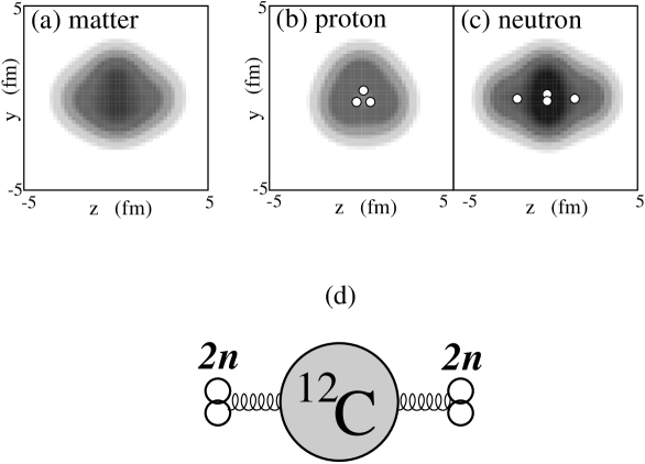
FIG. 9.: The density distribution of the ground state of ¹⁶C. The densities are integrated along the $x$-axis. (a)Matter density, (b) proton density, (c) neutron density are shown. The spatial configuration of the centers of single-particle Gaussian wave packets for protons and neutrons are also plotted by open circles in (b) and (c), respectively. Each circle consists of a spin-up nucleon and a spin-down nucleon. (d): The schematic figure for the configurations of the Gaussian centers in ¹⁶C written by $2n+^{12}$C+$2n$.

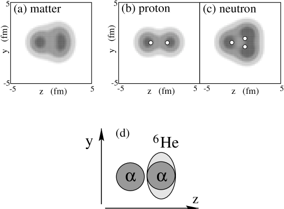
FIG. 10.: The density distribution of the ground state of ¹⁰Be. The densities are integrated along the $x$-axis. (a)Matter density, (b) proton density, (c) neutron density are shown. The spatial configuration of the centers of single-particle Gaussian wave packets for protons and neutrons are also plotted by open circles in (b) and (c), respectively. Each circle consists of a spin-up nucleon and a spin-down nucleon. (d): The schematic figure for the structure of ¹⁰Be with $\alpha+^{6}$He configuration.

FIG. 11.: Strength of the motion of the Gaussian centers in the response of ¹⁶C and ¹⁰Be with an instantaneous dipole field along $z$-axis. The strength is given by Fourier transform of positions of the Gaussian centers as shown in Eq.(23). We divide $A$ nucleons into some groups: $C_{1},C_{2},\cdots$ and sum up the components for nucleons in each group. (a)Motion of the Gaussian centers in ¹⁶C. $C_{1}$ consists of four valence neutrons, and $C_{2}$($C_{3}$) contains 6 protons(neutrons) in the ¹²C core. (b)Motion in ¹⁰Be. $C_{1}$, $C_{2}$ and $C_{3}$ consist of two valence neutrons, 4 protons, and 4 residual neutrons. (c)Relative motion between ⁴He($C_{1}$) and ⁶He($C_{2}$) clusters in ¹⁰Be. The dotted, dash-dotted, and solid lines correspond to $C_{1}$, $C_{2}$, and $C_{3}$.

We show the calculated photonuclear cross section in Fig.8. The shape of the strength function in the GDR region($E_{x}>17$ MeV) has a close relation with the deformation of the system. In the oblately deformed system such as ¹¹B and ²⁰C as well as ¹²C, the GDR splits in two part. The lower GDR peak has large transition strength. In the neutron-rich nucleus, ²⁰C, the excitation energy of the GDR is the lowest among the three nuclei. Also in the ⁸Be and ¹⁴Be with the prolate deformation, the GDR splits into two, but the higher GDR has larger strength in contrast to the oblate deformation. The lower resonance in ¹⁴Be exists at $E_{x}=15$ MeV. In triaxial nuclei such as ¹⁷B and ¹⁸C, the GDR consists of three peaks with 5 MeV of the energy splitting. However, considering spreading of the widths, three peaks may overlap to form a broad structure in the $E_{x}=15-30$ MeV. ¹⁰Be and ¹⁶C have the ground state with opposite deformations between proton and neutron densities. In spite of this unusual properties of the deformations, we can not find an abnormal feature in the dipole strength of the GDR region in these nuclei. As explained before, the remarkable soft peaks appear at $E_{x}=10-15$ MeV due to the motion of the valence nucleons against to the core, while the GDR at $E_{x}>17$ MeV arises from the vibration within the core. Therefore it is considered that the GDR may reflect mainly the features of the core nuclei instead of the deformations of the total system. In fact, the GDR of ¹⁰Be lies at a similar excitation energy to that of ⁸Be.

Below the GDR region, we find the significant strengths of the soft resonances in such neutron-rich nuclei as ¹⁰Be, ¹⁵B, ¹⁶C and ¹⁸C due to the excess neutrons. Especially, ¹⁰Be, ¹⁵B and ¹⁶C have the remarkable soft peaks, which are decoupled with the GDR. In the neutron-rich nuclei, the cluster sum rule[35] is a convenient measure to estimate the contribution of the motion of the excess neutrons in the dipole strengths[36]. Assuming clustering with a core and $N_{v}$ valence neutrons, we consider the core cluster with $Z_{1}=Z,N_{1}=N-N_{v}$ and the valence cluster with $Z_{2}=0,N_{2}=N_{v}$. The cluster sum rule is given as,

$$S_{\rm clust}=\frac{\hbar^{2}}{2m}\frac{9}{4\pi}\frac{(Z_{1}N_{2}-Z_{2}N_{1})^{2}}{A(Z_{1}+N_{1})(Z_{2}+N_{2})}e^{2}=\frac{\hbar^{2}}{2m}\frac{9}{4\pi}\frac{Z^{2}N_{v}^{2}}{A(A-N_{v})N_{v}}e^{2}.$$ (24)

This value is the remainder when one subtract the core contribution of the classical EWSR from the total $S(TRK)$ value. Consequently, $S_{\rm clust}$ is the margin which indicates the contribution of the excess neutrons. The integrated strength of the low-energy resonances should be compared with $S_{\rm clust}$ to see the softness and collectivity of the resonances due to the valence neutron motion against the core. In table III, the EWSR for the low-lying resonances are listed with the values of the classical TRK sum rule and the cluster sum rule($S_{\rm clust}$). In the derivation of the cluster sum rule $S_{\rm clust}$, the core cluster is assumed to be ⁸Be, ¹¹B, ¹²C and ¹⁶O, in Be, B, C and O isotopes, respectively. We show the EWSR values integrated up to $E_{x}<15$ MeV and $E_{x}<17$ MeV in the present results, and the EWSR with other calculations. The ratios of the EWSR to $S(TRK)$ and $S_{\rm clust}$ are shown in Figs.12(a) and 12(b), respectively. In C isotopes, $S(E1;E_{x}<17$ MeV) is the largest in ¹⁶C and it declines in further neutron-rich C isotopes. The present results of C isotopes well agree to the shell model calculations[13]. Also in B isotopes, the similar feature is found. Namely, $S(E1;E_{x}<17$ MeV) is the largest in ¹⁵B and it decreases in further neutron-rich nucleus ¹⁷B. The striking point is that the EWSR for the low-lying resonances is remarkably enhanced in the moderately neutron-rich nuclei with an appropriate number of excess neutrons, but it is suppressed in very neutron-rich nuclei. It is reasonable because the enhancement of the soft dipole strengths is due to the coherent motion of the valence neutrons relative to the core. It means that the decoupled collective modes appear based on the relative motion between the core and valence neutrons and the motion inside the core, in ¹⁵B and ¹⁶C. On the other hand, as the neutron skin develops in further neutron-rich nuclei $N>10$, the motion of the excess neutrons is not decoupled but they join the neutrons inside the core. As a result, in ¹⁷B and ²⁰C, the soft dipole mode is assimilated into the GDR, and the excitation energy of the GDR decreases. Also in ¹⁰Be, the EWSR for the low-lying resonances is significant as well as ¹⁵B and ¹⁶C. In these nuclei, the cluster sum rule value $S_{\rm clust}$ is almost exhausted by the calculated $S(E1;E_{x}<17$ MeV). In ¹⁴Be, the $S(E1;E_{x}<17$ MeV) is very large due to the peak at $E_{x}=16$ MeV. The reason for the enhanced $S(E1;E_{x}<17$ MeV) in ¹⁴Be is different from other nuclei(¹⁰Be,¹⁵B and ¹⁶C). In case of ¹⁴Be, the enhanced $S(E1;E_{x}<17$ MeV) does not originate in the soft resonance decoupled from the GDR, but the GDR for the longitudinal vibration itself contributes the EWSR for low-energy region because it becomes soft due to the prolate deformation with a developed neutron skin structure.

TABLE III.: The Energy-weighted sum rule for the soft dipole resonances. The energy weighted sum integrated up to $E_{x}<17$ MeV and $E_{x}<15$ MeV are shown in the fourth and fifth columns. The core cluster in the derivation of the cluster sum rule $S_{\rm clust}$ is ⁸Be, ¹¹B, ¹²C and ¹⁶O, in Be, B, C and O isotopes, respectively. The smoothing parameter is chosen to be $\Gamma=2.0$ MeV. The unit is $e^{2}$fm²MeV.

	$S(TRK)$	$S_{\rm clust}$	$S(E1)$
			$E_{x}<17$ MeV	$E_{x}<15$ MeV
8Be	29.7	$-$	0.3	0.2
10Be	35.6	5.9	4.3	4.0
14Be	42.4	12.7	19.0	3.1
12C	44.5	$-$	0.5	0.3
16C	55.6	11.1	8.3	6.9
18C	59.3	14.8	5.6	3.4
20C	62.3	17.8	2.3	1.6
11B	40.5	$-$	1.1	0.8
15B	49.4	9.0	8.2	6.4
17B	52.3	11.9	5.8	1.7
18O	65.9	6.6	4.0	1.5

FIG. 12.: The ratio of the EWSR integrated for the soft dipole resonances to $S(TRK)$ and $S_{\rm clust}$. Circles indicate the ratio for $S(E1;E_{x}<17$ MeV) and squares are for $S(E1;E_{x}<15$ MeV). The smoothing parameter is chosen to be $\Gamma=2.0$ MeV. The results of TDHF+ABC for $S(E1;E_{x}<15$ MeV) in Be isotopes are plotted by the symbols “$+$”. The symbols “$\times$” show the results of the shell model calculations for $S(E1;5<E_{x}<15$ MeV), $S(E1;E_{x}<14$ MeV), $S(E1;E_{x}<15$ MeV) in Be[15], C[17], and O[13], respectively.

VI Summary

We applied a method of the time-dependent AMD to dipole transitions in light neutron-rich nuclei. We investigated the $E1$ resonances in Be, B, and C isotopes. It was found that the remarkable peaks appear in ¹⁰Be, ¹⁵B, and ¹⁶C at $E_{x}=10-15$ MeV which almost exhaust the values of the cluster sum rule. These soft dipole resonances arise from the relative motion between excess neutrons and the core, which is decoupled with the motion inside the core. In other words, these soft resonances appear due to the excitation of the excess neutrons around the rather hard core. This nature of the neutron excitation and the inert core may have a link with such ground-band properties of the ¹⁶C as the unusually small $B(E2;2^{+}_{1}\rightarrow 0^{+}_{1})$[37], which has been recently investigated in theoretical and experimental studies [3, 38, 39, 40]. In further neutron-rich B and C isotopes with $N>10$, the strength for the soft dipole resonances declines compared with that of ¹⁵B and ¹⁶C. It is considered to be because the motion of the excess neutrons assimilates into the neutron motion within the core. As a result, the excitation energies of the GDR decrease with the enhancement of the neutron-skin. It is striking that the strength for the soft dipole resonances does not necessarily increase with the increase of the excess neutrons. Instead, the feature of the soft resonances rapidly changes depending on the proton and neutron numbers of the system. The key of the soft dipole resonance with a remarkable strength is how the coherent motion of the valence neutrons is decoupled with the motion inside the core.

The present method based on the time-dependent AMD is regarded as a kind of small-amplitude time-dependent Hartree-Fock calculations within the AMD model space. The point of the method is that we are able to study dipole resonances with the framework which can describe cluster aspect. In the AMD approach, the dipole excitations are expressed by the motion of single-particle Gaussian wave packets, because the expectation value of the dipole operator is related directly to the centers of the Gaussian wave packets. One of the advantages of the time-dependent AMD is that we can link the excitations with such collective modes as core vibration, core-neutron motion and inter-cluster motion, which should be important to understand the role of the excess neutrons in the dipole resonances.

Recently, extended methods of time-dependent mean-field calculations have been proposed and applied to the dipole transitions in neutron-rich nuclei. In the TDHF+ABC approach, which have been applied to deformed neutron-rich nuclei by Nakatsukasa and Yabana[18], the effects of continuum states are taken into account. Another method is the time-dependent density-matrix theory which has been applied to ²²O by incorporating two-body correlations [7]. In the present work, the contributions of continuum states are omitted, and the detailed descriptions of wave functions and two-body correlations should be insufficient, as the model space is a simple AMD wave function written by a Slater determinant of Gaussian wave packets. Therefore, we put an artificial smoothing parameter to simulate the width of the dipole resonances, because it is difficult to describe the escape and the spreading widths of the resonances in the present framework. Further extensions of the model must be essential to give quantitative discussions of the excitation energies and the strengths of the dipole resonances in nuclei near the drip line. It should be necessary to solve the remaining problem of the soft resonances in halo nuclei [4, 5, 6, 12, 14, 19, 21].

We comment that the usual AMD wave functions applied to the nuclear structure study are the advanced ones with some extensions such as the parity and spin projections, deformed Gaussian base and generator coordinate method [22, 34, 41, 42, 43], though the present AMD wave function is the simplest one with no extension. A combination of the time-dependent method and the extended AMD wave functions should be needed to include higher correlations beyond the present calculations, and also to obtain better description of the ground state properties. Moreover, interaction dependence of the dipole transitions is a remaining problem.

References

REFERENCES

- [1] Y. Kanada-En’yo, H. Horiuchi and A. Ono, Phys. Rev. C 52, 628 (1995); Y. Kanada-En’yo and H. Horiuchi, Phys. Rev. C 52, 647 (1995).
- [2] Y.Kanada-En’yo and H.Horiuchi, Phys.Rev. C 55, 2860 (1997).
- [3] Y.Kanada-En’yo Phys. Rev. C 71, 014310 (2005).
- [4] M.Honma, H.Sagawa Prog. Theor. Phys. 84, 494 (1990).
- [5] T.Hoshino, H.Sagawa and A.Arima, Nucl.Phys. A523, 228 (1991).
- [6] H.Sagawa, N.Takigawa, Nguyen van Giai Nucl.Phys. A543, 575 (1992).
- [7] M. Tohyama, Phys.Lett. 323B, 257 (1994).
- [8] I.Hamamoto, H.Sagawa and X.Z.Zhang, Phys.Rev. C 53, 765 (1996).
- [9] I.Hamamoto and H.Sagawa, Phys.Rev. C 53, R1492 (1996).
- [10] F.Catara, E.G.Lanza, M.A.Nagarajan and A.Vitturi, Nucl. Phys. A624, 449 (1997).
- [11] I. Hamamoto, H. Sagawa, and X. Z. Zhang, Phys. Rev. C 57, R1064 (1998).
- [12] T.Myo, A.Ohnishi and K.Kato, Prog. Theor. Phys. 99, 801 (1998)
- [13] H. Sagawa and T. Suzuki, Phys. Rev. C 59, 3116 (1999).
- [14] T.Suzuki, H.Sagawa and P.F.Bortignon Nucl. Phys. A662, 282 (2000).
- [15] H. Sagawa, T. Suzuki, H. Iwasaki and M. Ishihara, Phys. Rev. C 63, 034310 (2001).
- [16] G. Colo and P. F. Bortignon, Nucl. Phys. A969, 427 (2001).
- [17] T. Suzuki, H. Sagawa and K. Hagino, Phys. Rev. C 68, 014317 (2003).
- [18] T. Nakatsukasa and K. Yabana, Phys. Rev. C 71, 024301 (2005).
- [19] T.Nakamura et al., Phys. Lett. 394B, 11 (1997).
- [20] A. Leistenschneider et al., Phys. Rev. Lett. 86, 5442 (2001).
- [21] R.Palit et al., Phys. Rev. C 68, 034318 (2003).
- [22] Y. Kanada-En’yo and H. Horiuchi, Prog. Theor. Phys. Suppl.142, 205 (2001).
- [23] A.Ono, H.Horiuchi, T.Maruyama and A.Ohnishi, Phys. Rev. Lett. 68, 2898 (1992).
- [24] A.Ono, H.Horiuchi, T.Maruyama and A.Ohnishi, Prog. Theor. Phys. 87, 1185 (1992).
- [25] Y. Kanada-En’yo, M. Kimura and H. Horiuchi, Comptes rendus Physique Vol.4, 497 (2003).
- [26] T. Ando, K.Ikeda, and A. Tohsaki, Prog. Theor. Phys. 64, 1608 (1980).
- [27] N. Yamaguchi, T. Kasahara, S. Nagata, and Y. Akaishi, Prog. Theor. Phys. 62, 1018 (1979); R. Tamagaki, Prog. Theor. Phys. 39, 91 (1968).
- [28] M. W. Kirson, Nucl. Phys. A301, 93 (1978).
- [29] P. Ring and P. Schuck, The Nuclear Many-Body Problem (Springer-Verlag, New York, 1980).
- [30] R. E. Pywell et al., Phys. Rev. C 32, 384 (1985).
- [31] J. G. Woodworth et al., Phys. Rev. C 19, 1667 (1979).
- [32] S. C. Fults, J. T. Caldwell, B. L. Berman, R. L. Bramblett and R. R. Harvey, Phys. Rev. 143, 790 (1966).
- [33] B. L. Berman, D. D. Faul, R. A. Alvarez and P. Meyer, Phys. Rev. Lett. 36, 1441 (1976).
- [34] Masaaki Kimura, Yoshio Sugawa and Hisashi Horiuchi, Prog. Theor. Phys. 106, 115 (2001).
- [35] Y. Alhassid, M. Gai and G. F. Bertsch, Phys. Rev. Lett. 49, 1482 (1982).
- [36] H. Sagawa and M. Honma, Phys. Lett. 251B, 17 (1990).
- [37] N. Imai et al., Phys. Rev. Lett. 92, 062501 (2004).
- [38] Z. Elekes et al., Phys. Lett. 586B, 34 (2004).
- [39] H. Sagawa, X. R. Zhou, and X. Z. Zhang and T. Suzuki, Phys. Rev. C 70, 054316 (2004).
- [40] M.Takashina, Y.Kanada-En’yo and Y.Sakuragi, Phys. Rev. C 71, 054602 (2005).
- [41] Y. Kanada-En’yo, Phys. Rev. Lett. 81, 5291 (1998).
- [42] N. Itagaki and S. Aoyama, Phys. Rev. C 61, 024303 (2000).
- [43] G.Thiamova, N.Itagaki, T.Otsuka and K.Ikeda, Nucl. Phys. A719, 312c (2003).