Two-Body Electrodisintegration of ³He at High Momentum Transfer

Abstract

The ³He$(e,e^{\prime}p)$$d$ reaction is studied using an accurate three-nucleon bound state wave function, a model for the electromagnetic current operator including one- and two-body terms, and the Glauber approximation for the treatment of final state interactions. In contrast to earlier studies, the profile operator in the Glauber expansion is derived from a nucleon-nucleon scattering amplitude, which retains its full spin and isospin dependence and is consistent with phase-shift analyses of two-nucleon scattering data. The amplitude is boosted from the center-of-mass frame, where parameterizations for it are available, to the frame where rescattering occurs. Exact Monte Carlo methods are used to evaluate the relevant matrix elements of the electromagnetic current operator. The predicted cross section is found to be in quantitative agreement with the experimental data for values of the missing momentum $p_{\rm m}$ in the range (0–700) MeV/c, but underestimates the data at $p_{\rm m}\simeq 1$ GeV/c by about a factor of two. However, the longitudinal-transverse asymmetry, measured up to $p_{\rm m}\simeq$ 600 MeV/c, is well reproduced by theory. A critical comparison is carried out between the results obtained in the present work and those of earlier studies.

I Introduction

Recent experiments at JLab have yielded beautiful data for the ³He$(e,e^{\prime}p)$$d$ cross section and longitudinal-transverse asymmetry up to missing momenta $p_{\rm m}\simeq 1.1$ and 0.6 GeV/c Rvachev05 , respectively, and the three-body breakup cross section ³He$(e,e^{\prime}p)$$p$$n$ for missing momenta and energies ($E_{\rm m}$) in the range $p_{\rm m}$ up to 0.84 GeV/c and $E_{\rm m}$ up to 140 MeV Benmokhtar05 . These data have spurred renewed interest in these reactions, which has led to a series of papers Ciofi05 ; Ciofi05a ; Laget05 ; Laget05a , dealing with the theoretical description of the proton-knockout mechanism and, in particular, with the treatment of final state interactions (FSI) at GeV energies.

In the present work, we contribute to this effort. As in Refs. Ciofi05 ; Ciofi05a we adopt the Glauber approximation to describe the rescattering processes between the struck proton and the nucleons in the recoiling deuteron. However, in contrast to the studies of Refs. Ciofi05 ; Ciofi05a ; Laget05 ; Laget05a , we retain the full spin and isospin dependence of the nucleon-nucleon ($N$$N$) scattering amplitude from which the Glauber profile operator is derived, and do not make use of the factorization approximation, which allows one to write the $(e,e^{\prime}p)$ cross section on a nucleus in terms of a proton cross section times a distorted spectral function. A number of issues pertaining to the parameterization of the $N$$N$ amplitude, and its boosting from the center-of-mass (c.m.) frame to the frame in which rescattering occurs, are discussed in considerable detail.

The spin dependence of the $N$$N$ amplitudes will turn out to play an important role in the high $p_{\rm m}$ region where double rescattering effects become dominant. It is not clear that one is justified in ignoring it, particularly in the analysis of experiments, such as the ⁴He$(\vec{e},e^{\prime}\vec{p}\,)$³H reaction Strauch03 , in which the polarizations of the ejected proton are measured Lava04 .

The present paper is organized as follows. In Sec. II we briefly review the bound-state wave functions and the model for the electromagnetic current operator, while in Sec. III the Glauber approximation, the profile operator, and the parameterization for the $N$$N$ scattering amplitude are discussed. Next, in Sec. IV, the relevant formulae for the $(e,e^{\prime}p)$ cross section and their limits in the plane-wave-impulse-approximation (PWIA) are summarized, while in Sec. V the Monte Carlo method, as implemented in the present calculations, is described. Finally, in Sec. VI we present a detailed discussion of the results, including a critical comparison between the present and earlier studies, while in Sec. VII we summarize our conclusions.

II Wave functions and currents

In this section we briefly describe the ³He wave function and the model for the nuclear electromagnetic current. The discussion is rather cursory, since both these aspects of the calculations presented in this work have already been reviewed in considerable detail in a number of earlier papers. References to these are included below.

II.1 Bound-state wave functions

The ground states of the $A$=3 nuclei are represented by variational wave functions, derived from a realistic Hamiltonian consisting of the Argonne $v_{18}$ two-nucleon ($N$$N$) Wiringa95 and Urbana-IX three-nucleon ($N$$N$$N$) Pudliner95 interactions—the AV18/UIX Hamiltonian model—with the correlated hyperspherical-harmonics (CHH) method Kievsky93 . The high accuracy of the CHH wave functions is well documented Nogga03 , as is the quality of the AV18/UIX Hamiltonian in successfully and quantitatively accounting for a wide variety of three-nucleon bound-state properties and reactions, ranging from binding energies, charge radii, and elastic form factors Nogga03 ; Marcucci98 ; Carlson98 to low-energy radiative and weak capture cross sections and polarization observables Marcucci04 , to the quasi-elastic response in inclusive $(e,e^{\prime})$ scattering at intermediate energies Carlson00 .

II.2 Electromagnetic current operator

The nuclear electromagnetic current includes one- and two-body terms,

$$\rho({\bf q}) = \sum_{i=1}^{A}\rho_{i}({\bf q})+\sum_{i<j=1}^{A}\rho_{ij}({\bf q})\ ,$$ (1)

$${\bf j}({\bf q}) = \sum_{i=1}^{A}{\bf j}_{i}({\bf q})+\sum_{i<j=1}^{A}{\bf j}_{ij}({\bf q})\ .$$ (2)

The one-body current and charge operators have the form recently derived by Jeschonnek and Donnelly Jeschonnek98 from an expansion of the covariant single-nucleon current, in which only terms dependent quadratically on the initial nucleon momentum (and higher order terms) are neglected. In momentum space, they are explicitly given by

$$\rho_{i}({\bf q})=\frac{q}{Q}G_{E}+\frac{\rm i}{\sqrt{1+\eta}}\frac{1}{2m^{2}}\left(G_{M}-\frac{1}{2}G_{E}\right){\bm{\sigma}}_{i}\cdot({\bf q}\times{\bf p}_{i})\ ,$$ (3)

$${\bf j}_{i}({\bf q})=\frac{Q}{q}\left[\frac{{\bf p}_{i}}{m}\left(G_{E}+\frac{\eta}{2}G_{M}\right)-\frac{\rm i}{2m}G_{M}\left({\bf q}\times{\bm{\sigma}}_{i}+\frac{\omega}{2m}{\hat{\bf q}}\cdot{\bm{\sigma}}_{i}\,\hat{\bf q}\times{\bf p}_{i}\right)\right]\ ,$$ (4)

where ${\bf q}$ ($\omega$) is the virtual photon three-momentum (energy) transfer, $Q$ is the four-momentum transfer with $Q^{2}$=$q^{2}-\omega^{2}$ $>0$, $\eta$ is defined as $\eta\equiv Q^{2}/(4m^{2})$, $m$ being the nucleon mass, and ${\bf p}_{i}$ and ${\bm{\sigma}}_{i}$ are the momentum and spin operators of nucleon $i$, respectively. The nucleon Sachs form factors $G_{E}$ and $G_{M}$ are defined as

$$G_{E/M}=\frac{1}{2}\left[(G_{Ep/Mp}+G_{En/Mn})+\tau_{i,z}\,(G_{Ep/Mp}-G_{En/Mn})\right]\ ,$$ (5)

where the $Q^{2}$ dependence is understood, and $\tau_{z}$ is the $z$-component of the isospin. The Höhler parameterization Hohler76 is used for the proton and neutron electric and magnetic form factors $G_{Ep/En}$ and $G_{Mp/Mn}$.

The form adopted above for the one-body currents is well suited for dealing with processes in which the energy transfer may be large (i.e., the ratio of four- to three-momentum transfer $(Q/q)^{2}$ is not close to one) and the initial momentum of the nucleon absorbing the virtual photon is small. Thus, its use is certainly justified in quasi-elastic kinematics for moderate values of the missing momentum. Note that in the limit $(Q/q)^{2}\simeq 1$ one recovers the standard non-relativistic expressions for the impulse-approximation currents (including the spin-orbit correction to the charge operator).

The two-body charge, $\rho_{ij}({\bf q})$, and current, ${\bf j}_{ij}({\bf q})$, operators consist of a “model-independent”part, that is constructed from the $N$$N$ interaction (the AV18 in the present case), and a “model-dependent”one, associated with the excitation of nucleons to $\Delta$ resonances (for ${\bf j}_{ij}$ only) and $\rho\pi\gamma$ and $\omega\pi\gamma$ transitions (for a review, see Ref. Carlson98 and references therein). Improvements in the construction of the model-independent two-body currents originating from the momentum-dependent terms of the $N$$N$ interaction have been recently reported in Ref. Marcucci05 . In this latter work, three-body currents associated with $N$$N$$N$ interactions have also been derived. Both these refinements, however, are expected to have little impact on the results of the present study, and therefore are not considered any further.

The present model for two-body charge and current operators is quite realistic at small momentum transfers. However, for processes involving momentum and energy transfers of order 1 GeV, such as the ³He($e,e^{\prime}p$)$d$ reaction under consideration here for which $q$=1.50 GeV/c and $\omega$=0.84 GeV, it is likely to have additional corrections.

III Final state interactions: Glauber approximation

In the kinematics considered in Sec. VI, the proton lab kinetic energies are typically of the order 0.5 GeV or larger. These energies are obviously beyond the range of applicability of $N$$N$ interaction models, such as the AV18, which are constrained to reproduce $N$$N$ elastic scattering data up to the pion production threshold. At higher energies, $N$$N$ scattering becomes strongly absorptive with the opening of particle production channels. Indeed, the $p$$p$ inelastic cross section at 0.5 GeV increases abruptly from about 2 mb to 30 mb, and remains essentially constant for energies up to several hundred GeV Lechanoine93 .

On the other hand, the small momentum transfer which characterizes scattering processes at high energies makes the Glauber approximation Glauber59 particularly well suited in this regime. Another advantage is its reliance on a $N$$N$ scattering amplitude, which is fitted to data. It is the approach we adopt in the present work to describe the wave function of the final $p$+($A-1$) system as

$$\psi(p+^{(A-1)}\!f;{\rm GLB})=\frac{1}{\sqrt{A}}\sum_{\cal P}\epsilon_{\cal P}\,G(A;1\dots A-1)\,{\rm e}^{{\rm i}{\bf p}\cdot{\bf r}_{A}}\chi_{\sigma}(A;p)\,{\rm e}^{{\rm i}{\bf p}_{f}\cdot{\bf R}_{1\dots A-1}}\phi_{\sigma_{f}}(1\dots A-1;f)\ ,$$ (6)

where $\chi_{\sigma}(p)$ represents a proton in spin state $\sigma$, $\phi_{\sigma_{f}}(f)$ denotes the wave function of the ($A-1$)-system with spin projection $\sigma_{f}$, and ${\bf R}_{1\dots A-1}$ is the center-of-mass position vector of the $A-1$ nucleons in this cluster. The sum over permutations $\cal P$ of parity $\epsilon_{\cal P}$ ensures the overall antisymmetry of $\psi(p+^{(A-1)}\!f;{\rm GLB})$.

The operator $G(A;1\dots A-1)$ inducing final-state-interactions (FSI) can be derived from an analysis of the multiple scattering series by requiring that the struck (fast) nucleon (nucleon $A$) moves in a straight-line trajectory (that is, it is undeflected by rescattering processes), and that the nucleons in the residual system (nucleons $1,\dots,A-1$) act as fixed scattering centers Wallace81 ; Benhar00 (the so-called frozen approximation). It is expanded as

$$G=1+\sum_{n=1}^{A-1}(-)^{n}G^{(n)}\ ,$$ (7)

where $G^{(n)}$ represents the $n^{\rm th}$ rescattering term, and therefore for an $A$-body system up to $A-1$ rescattering terms are generally present. The leading single-rescattering term reads

$$G^{(1)}(A;1\dots A-1)=\sum_{i=1}^{A-1}\theta(z_{iA})\,\Gamma_{iA}({\bf b}_{iA};s_{iA})\ ,$$ (8)

where $z_{iA}$ and ${\bf b}_{iA}$ denote the longitudinal and transverse components of ${\bf r}_{i}-{\bf r}_{A}$ relative to $\hat{\bf p}$, the direction of the nucleon momentum,

$$z_{iA}\equiv{\hat{\bf p}}\cdot({\bf r}_{i}-{\bf r}_{A})\ ,\qquad{\bf r}_{i}-{\bf r}_{A}\equiv{\bf b}_{iA}+z_{iA}\,{\hat{\bf p}}\ ,$$ (9)

and the step-function $\theta(x)$, $\theta(x)=1$ if $x>0$, prevents the occurrence of backward scattering for the struck nucleon. The “profile operator”$\,\Gamma_{iA}$, to be discussed below, is related to the Fourier transform of the $N$$N$ scattering amplitude at the invariant energy $\sqrt{s_{iA}}$.

The double-rescattering term, relevant for the present study of the ³He($e,e^{\prime}p$)$d$ reaction, is given by

$$G^{(2)}(A;1\dots A-1)=\sum_{i\neq j=1}^{A-1}\theta(z_{ij})\,\theta(z_{jA})\,\Gamma_{iA}({\bf b}_{iA};s_{iA})\,\Gamma_{jA}({\bf b}_{jA};s_{jA})\ ,$$ (10)

where the product of $\theta$-functions ensures the correct sequence of rescattering processes in the forward hemisphere. For example, if $z_{j}-z_{A}>0$ and $z_{i}-z_{j}>0$, then nucleon $A$ scatters first from nucleon $j$ and then from nucleon $i$. Note that the operators $\Gamma_{iA}$ and $\Gamma_{jA}$ do not generally commute.

III.1 The profile operator $\Gamma_{ij}$

At this stage it is useful to specify the kinematics of the various rescattering processes occurring in the Glauber expansion. Specializing to the ³He($e,e^{\prime}p$)$d$ reaction of interest here, the single- and double-rescattering terms are illustrated schematically in Fig. 1. In this figure, nucleon 3 denotes the knocked-out nucleon with momentum ${\bf p}_{3}$=${\bf p}$ and energy $E_{3}$=$E$ in the lab frame, while nucleons 1 and 2, making up the deuteron, have momenta ${\bf p}_{1}$ and ${\bf p}_{2}$, respectively, with ${\bf p}_{1}$+${\bf p}_{2}$=${\bf p}_{d}$ (again, in the lab frame). The black solid circle represents the $N$$N$ scattering amplitude. In the single-rescattering case, the $N$$N$ amplitudes in the two terms (panel a) of Fig. 1 only shows one of them) are evaluated at the invariant energies $\sqrt{s_{i3}}$, $i$=1,2, with

$$s_{i3} = (E_{i}+E_{3})^{2}-({\bf p}_{i}+{\bf p}_{3})^{2}$$ (11)

$$\simeq 2\,m^{2}+E\,\sqrt{{\bf p}_{d}^{2}+4\,m^{2}}-{\bf p}\cdot{\bf p}_{d}\ ,$$

where in the second line it has been assumed that i) the nucleons are on their mass shells, and ii) nucleons 1 and 2 in the recoiling deuteron share its momentum equally, ${\bf p}_{i}\simeq{\bf p}_{d}/2$. The momenta of nucleon 3 and nucleon $i$, $i$=1,2, after rescattering are ${\bf p}-{\bf k}$ and ${\bf p}_{d}/2+{\bf k}$, where ${\bf k}$ denotes the momentum transfer. The spectator nucleon ($j\not=i$) has momentum ${\bf p}_{d}/2$. Thus, the “rescattering frame”we refer to in the following is defined as that in which nucleon 3 (nucleon $i$) have initial and final momenta ${\bf p}$ and ${\bf p}-{\bf k}$ (${\bf p}_{d}/2$ and ${\bf p}_{d}/2+{\bf k}$), respectively.

In the case of double rescattering, panel b) of Fig. 1, a similar analysis can be carried out. In particular, it leads in the eikonal limit to the approximation in which both $N$$N$ amplitudes are evaluated at the invariant energies $\sqrt{s_{13}}\simeq\sqrt{s_{23}}$, as obtained in Eq. (11).

The profile operator $\Gamma_{ij}$ is related to the $N$$N$ scattering amplitude in the rescattering frame, denoted as $F_{ij}({\bf k};s)$, via the Fourier transform

$$\Gamma_{ij}({\bf b};s)=\frac{1}{2\pi{\rm i}\,p}\int{\rm d}^{2}{\bf k}\,{\rm e}^{-{\rm i}{\bf k}\cdot{\bf b}}F_{ij}({\bf k};s)\ ,$$ (12)

where, in the eikonal limit, the momentum transfer ${\bf k}$ is perpendicular to ${\bf p}$. The isospin symmetry of the strong interactions allows one to express $F_{ij}$ as

$$F_{ij}=F_{ij,+}+F_{ij,-}{\bm{\tau}}_{i}\cdot{\bm{\tau}}_{j}\ ,$$ (13)

where the $F_{ij,\pm}$ are related to the physical amplitudes for $p$$p$ and $p$$n$ scattering via

$$F_{ij,\pm}=\frac{F^{pp}_{ij}\pm F^{pn}_{ij}}{2}\ .$$ (14)

Available parameterizations of the $p$$p$ and $p$$n$ amplitudes are given in the c.m. frame Wallace81 , and therefore one needs to boost these from the c.m. to the rescattering frame. In the discussion that follows, the general form of the c.m. amplitude and its parameterization are described first, while the boosting procedure adopted in the present work is illustrated next.

III.2 The $N$$N$ scattering amplitude in the c.m. frame

It is well known that the most general form for the $N$$N$ scattering amplitude in the c.m. frame reads (see Refs. Lechanoine93 ; Wallace81 and references therein)

$$(2{\rm i}\,\overline{p})^{-1}\,\overline{F}^{\,NN}_{ij}(\,\overline{{\bf k}},s)=\sum_{m=1}^{5}\overline{F}^{\,NN}_{m}(s,\overline{{\bf k}}^{\,2})\overline{O}^{\,m}_{ij}\ ,$$ (15)

where $\overline{\bf p}$ and $\overline{\bf p}^{\,\prime}$ denote the initial and final nucleon momenta, respectively, the $\overline{F}^{\,NN}_{m}$’s are functions of the invariant energy $\sqrt{s}$ and momentum transfer $\overline{\bf k}^{\,2}$ (with $\overline{\bf k}=\overline{\bf p}-\overline{\bf p}^{\,\prime}$), and a possible choice for the five operators $\overline{O}^{\,m}_{ij}$, especially convenient for our present purposes, is that given in Ref. Wallace81 ,

$$\overline{O}^{\,m=1,\dots,5}_{ij}=1\,,\,{\bm{\sigma}}_{i}\cdot{\bm{\sigma}}_{j}\,,\,{\rm i}\,({\bm{\sigma}}_{i}+{\bm{\sigma}}_{j})\cdot\overline{\bf k}\times{\overline{\bf e}}\,,\,{\bm{\sigma}}_{i}\cdot\overline{\bf k}\,{\bm{\sigma}}_{j}\cdot\overline{\bf k}\,,\,{\bm{\sigma}}_{i}\cdot{\overline{\bf e}}\,{\bm{\sigma}}_{j}\cdot{\overline{\bf e}}\ .$$ (16)

Here the unit vector ${\overline{\bf e}}$ is defined as ${\overline{\bf e}}\equiv(\overline{\bf p}+\overline{\bf p}^{\,\prime})/\mid\overline{\bf p}+\overline{\bf p}^{\,\prime}\mid$ ($\simeq\overline{\bf p}/\mid\overline{\bf p}\mid$ in the eikonal limit), and the overline on the various quantities in the equations above is to indicate that they are given in the c.m. frame. The factor $(2{\rm i}\,\overline{p})^{-1}$ in the l.h.s. of Eq. (15) is conventional.

The functions $\overline{F}^{NN}_{m}$ are parameterized as

$$\overline{F}^{\,NN}_{m}(s,\overline{\bf k}^{\,2})=\overline{\alpha}^{NN}_{m}\!(s)\,\,{\rm exp}\left[-\overline{\beta}^{NN}_{m}\!(s)\,\overline{\bf k}^{\,2}\right]\ ,$$ (17)

where the $\overline{\alpha}^{NN}_{m}\!(s)$ and $\overline{\beta}^{NN}_{m}\!(s)$ coefficients depend on $s$ and are generally complex; in particular, the forward, spin-independent amplitude $\overline{F}^{\,NN}_{1}(s,0)$ is given by $\overline{F}^{\,NN}_{1}(s,0)=\sigma^{NN}(1-{\rm i}\rho^{NN})/(8\pi)$ (an invariant quantity), where $\sigma^{NN}$ is the total cross section and $\rho^{NN}$ is the ratio of the imaginary to the real part of $\overline{F}^{\,NN}_{1}(s,0)$. In the present work these coefficients are taken from Tables III and IV of Ref. Wallace81 : they were obtained by fitting $N$$N$ amplitudes derived from the phase-shift analysis of the VPI group Arndt82 . The tabulations are for $s$ values in the range (3.92–5.09) GeV, corresponding to lab kinetic energies (210–831) MeV, for both $p$$p$ and $p$$n$ scattering. A detailed assessment of the accuracy and limitations of these parameterizations (of course, in relation to the $N$$N$ scattering data available up to 1981) can be found in Ref. Wallace81 . Here, it suffices to note only that they are reasonably accurate for the central and single spin-flip terms for $\overline{{\bf k}}^{\,2}$ up to $\simeq 0.1$ (GeV/c)²; however, double spin-flip terms are not well fitted by (single) Gaussian functions.

It would be desirable to update and improve the parameterizations of Ref. Wallace81 by using phase-shift analyses based on the current $N$$N$ database. Unfortunately, at the higher lab energies of interest here (say, above 500 MeV) the increase in the size of this database has been rather modest since the early 1980’s.

It is worth pointing out that all previous Glauber calculations of $A$($e,e^{\prime}p)$ processes we are aware of have ignored the double spin-flip terms in the scattering amplitude, corresponding to $m$=2, 4, and 5 in Eq. (15); indeed, most have only included the spin independent term (see, for example, Refs. Benhar00 ; Ryckebusch03 ; Ciofi05 ; Ciofi05a ).

Finally, note that, if the amplitude in Eq. (15) were to consist only of the scalar term ($m$=1), then the transformation to the lab frame would be unnecessary, since $(2{\rm i}\,\overline{p})^{-1}\,\overline{F}^{\,NN}_{ij}$ would be an invariant function of $s$ and the four-momentum transfer squared $t$=$-\overline{\bf k}^{\,2}$. However, the presence of the spin-dependent terms spoils this simplicity.

III.3 Boosting the $N$$N$ scattering amplitude to the rescattering frame

In order to boost the $N$$N$ scattering amplitude from the c.m. to the rescattering frame, we adopt the procedure described in Ref. McNeil83 , although its practical implementation in the present work is approximate for reasons discussed below. First, an invariant representation of the amplitude is introduced in terms of scalar, vector ($\gamma^{\mu}$), tensor ($\sigma^{\mu\nu}$), pseudoscalar ($\gamma^{5}$), and axial vector ($\gamma^{5}\gamma^{\mu}$) combinations of Dirac matrices:

$${\cal F}^{NN}_{ij}=\sum_{m=1}^{5}{\cal F}_{m}^{NN}(s,t)\Lambda_{ij}^{m}\ ,$$ (18)

where the five operators $\Lambda_{ij}^{m}$ are defined as

$$\Lambda_{ij}^{m=1,\dots,5}=1\,,\,\gamma_{i}^{\mu}\gamma_{j,\mu}\,,\,\sigma_{i}^{\mu\nu}\sigma_{j,\mu\nu}\,,\,\gamma_{i}^{5}\gamma_{j}^{5}\,,\,\gamma^{5}_{i}\gamma_{i}^{\mu}\gamma^{5}_{j}\gamma_{j,\mu}\ .$$ (19)

The relation between the functions ${\cal F}^{NN}_{m}$ and $\overline{F}^{\,NN}_{m}$ in the c.m. frame follows by noting that

$$\overline{u}_{\sigma_{i}^{\prime}}(\overline{\bf p}^{\,\prime})\overline{u}_{\sigma_{j}^{\prime}}(-\overline{\bf p}^{\,\prime}){\cal F}^{NN}_{ij}u_{\sigma_{i}}(\overline{\bf p})u_{\sigma_{j}}(-\overline{\bf p})=\chi_{\sigma_{i}^{\prime}}^{\dagger}\chi_{\sigma_{j}^{\prime}}^{\dagger}\left[(2{\rm i}\,\overline{p})^{-1}\,\overline{F}^{\,NN}_{ij}(\,\overline{{\bf k}},s)\right]\chi_{\sigma_{i}}\chi_{\sigma_{j}}\ ,$$ (20)

where the $u_{\sigma}$ are (positive-energy) Dirac spinors with $\overline{u}_{\sigma}\equiv u_{\sigma}^{\dagger}\gamma^{0}$, and $\chi_{\sigma}$ are two-component Pauli spinors. This leads in the eikonal limit $\overline{\bf p}\simeq\overline{\bf p}^{\,\prime}$ to

$${\cal F}^{NN}_{m}(s,\overline{\bf k}^{\,2})=\sum_{n=1}^{5}\overline{M}_{mn}(\overline{p},\overline{\bf k}^{\,2})\,\overline{F}^{\,NN}_{n}(s,\overline{\bf k}^{\,2})\ ,$$ (21)

where the matrix $\overline{M}$ is the inverse of that given in Tables I and II of Ref. McNeil83 . In fact, the $\overline{\bf k}^{\,2}$ dependence in the matrix $\overline{M}$ is neglected, i.e. $\overline{M}\equiv\overline{M}(\overline{p},0)$, in the present work, which allows one to write ${\cal F}^{NN}_{m}$, $m=1,\dots,5$, as a linear combination of terms, each having, as far as the momentum transfer dependence is concerned, the same Gaussian functional form as $\overline{F}^{\,NN}_{n}$. This turns out to be convenient when performing the Fourier transform in Eq. (12).

Next, having determined the functions ${\cal F}^{NN}_{m}$, the scattering amplitude in the rescattering frame is obtained from

$$\chi_{\sigma_{i}^{\prime}}^{\dagger}\chi_{\sigma_{j}^{\prime}}^{\dagger}\left[(2{\rm i}\,p)^{-1}\,F^{NN}_{ij}({\bf k},s)\right]\chi_{\sigma_{i}}\chi_{\sigma_{j}}=\overline{u}_{\sigma_{i}^{\prime}}({\bf p}-{\bf k})\overline{u}_{\sigma_{j}^{\prime}}({\bf p}_{d}/2+{\bf k}){\cal F}^{NN}_{ij}u_{\sigma_{i}}({\bf p})u_{\sigma_{j}}({\bf p}_{d}/2)\ ,$$ (22)

where in practice the dependence upon ${\bf p}_{d}/2$ in the spinors of particle $j$ has been neglected (in this limit, the rescattering and lab frames coincide). This approximation is justified at low $p_{d}$ (corresponding to low missing momenta), but is clearly unsatisfactory at high $p_{d}$ ($p_{d}\simeq 1$ GeV/c in the experiment of Ref. Rvachev05 ). The resulting $F^{NN}_{ij}({\bf k},s)$ has central, single and double spin-flip terms.

The approximations above—neglecting the dependence of the matrix $\overline{M}$ on the momentum transfer in Eq. (21), and the momentum ${\bf p}_{d}/2$ in Eq. (22)–made in boosting the $N$$N$ amplitude from the c.m. to the rescattering frame, have been dictated by computational convenience rather than by necessity, and could be removed. This latter task, however, is beyond the scope of the present work.

IV Cross section and response functions

To set the stage for the discussions that follow in later sections, it is helpful to give the expression of the five-fold differential cross section for the ${}^{A}i$$(e,e^{\prime}p)$${}^{(A-1)}\!f$ process (for a derivation, see Ref. Raskin89 ):

$$\frac{{\rm d}^{5}\sigma}{{\rm d}E_{e}^{\prime}{\rm d}\Omega_{e}^{\prime}{\rm d}\Omega}=p\,E\,\sigma_{\rm Mott}f_{\rm rec}\frac{m}{E}\frac{m_{f}}{E_{f}}\left[v_{L}R_{L}+v_{T}R_{T}+v_{LT}R_{LT}{\rm cos}(\phi)+v_{TT}R_{TT}{\rm cos}(2\phi)\right]\ ,$$ (23)

where $E_{e}^{\prime}$ is the energy of the final electron, $\Omega_{e}^{\prime}$ and $\Omega$ are the solid angles of, respectively, the final electron and knocked-out proton, $m_{f}$ is the rest mass of the ($A$–1)-cluster (assumed bound here), ${\bf p}$ and $E$ (${\bf p}_{f}$ and $E_{f}$) are the momentum and energy of the proton (($A$–1)-cluster) in the lab system, $\phi$ is the angle between the electron scattering plane and the plane defined by the momenta ${\bf q}$ and ${\bf p}$, and the recoil factor $f_{\rm rec}$, or rather its inverse, is defined as

$$f^{-1}_{\rm rec}=\Bigg{|}1-\frac{p_{f}E}{pE_{f}}\hat{\bf p}\cdot\hat{\bf p}_{f}\Bigg{|}\ .$$ (24)

The Mott cross section $\sigma_{\rm Mott}$ and the coefficients $v_{\alpha}$, $\alpha$=$L$, $T$, $LT$, and $TT$, are defined in terms of the electron kinematical variables, as given in Eqs. (2.19) and (2.27$a$)–(2.27$d$) of Ref. Raskin89 (note, however, that in that work $Q^{2}$ is taken to be negative).

The response functions $R_{\alpha}$ involve matrix elements of the charge and current operators between the initial ${}^{A}i$ and final $p$+${}^{(A-1)}\!f$ nuclear states, and depend on the momenta $q$ and $p$, the angle $\theta$ between them, and the energy transfer $\omega$. In a schematic notation, they are given by

$$R_{L} = |\langle p+^{(A-1)}\!f\mid\rho(q\hat{\bf z})\mid^{A}i\rangle|^{2}\ ,$$ (25)

$$R_{T} = |\langle p+^{(A-1)}\!f\mid{\bf j}_{\perp}(q\hat{\bf z})\mid^{A}i\rangle|^{2}\ ,$$ (26)

$$R_{LT} = 2\sqrt{2}\,\langle p+^{(A-1)}\!f\mid\rho(q\hat{\bf z})\mid^{A}i\rangle^{*}\,\langle p+^{(A-1)}\!f\mid j_{x}(q\hat{\bf z})\mid^{A}i\rangle\ ,$$ (27)

$$R_{TT} = -|\langle p+^{(A-1)}\!f\mid j_{x}(q\hat{\bf z})\mid^{A}i\rangle|^{2}+|\langle p+^{(A-1)}\!f\mid j_{y}(q\hat{\bf z})\mid^{A}i\rangle|^{2}\ ,$$ (28)

where the $z$-axis has been taken along ${\bf q}$, which also defines the spin-quantization axis, ${\bf j}_{\perp}$ denotes the components of the current transverse to ${\bf q}$, and the average over the initial, and sum over the final, spin projections are understood.

IV.1 The plane-wave-impulse-approximation

In the plane-wave-impulse-approximation (PWIA) limit, in which final-state interactions (FSI) effects between the knocked-out proton and the nucleons in the recoiling cluster are ignored (i.e., the operator $G$ in Eq. (6) is set to one), the response functions $R^{\rm PWIA}_{\alpha}$ can be expressed, neglecting two-body terms in the electromagnetic current operator, as

$$R^{\rm PWIA}_{\alpha}=r^{p}_{\alpha}\,N_{pf}(p_{\rm m})\ ,$$ (29)

where the $r^{p}_{\alpha}$ denote appropriate combinations of kinematical factors with the proton electric and magnetic form factors—those corresponding to the one-body currents of Sec. II.2 are listed in Appendix A—and $N_{pf}(p_{\rm m})$ is the $p$+($A$–1)-cluster momentum distribution, defined as

$$N_{pf}(p_{\rm m})=\frac{1}{2J_{i}+1}\,\sum_{\sigma_{i},\sigma,\sigma_{f}}|A^{pf}_{\sigma,\sigma_{f};\sigma_{i}}({\bf p}_{\rm m})|^{2}\ ,$$ (30)

with

$$A^{pf}_{\sigma,\sigma_{f};\sigma_{i}}({\bf p}_{\rm m})=\sqrt{\frac{A}{(2\pi)^{3}}}\,\int{\rm d}{\bf r}_{1}\dots{\rm d}{\bf r}_{A}\,{\rm e}^{-{\rm i}{\bf p}_{\rm m}\cdot({\bf r}_{A}-{\bf R}_{1\dots A-1})}\,\chi^{\dagger}_{\sigma}(A;p)\,\phi^{\dagger}_{\sigma_{f}}(1\dots A-1;f)\,\psi_{\sigma_{i}}(1\dots A;i)\ .$$ (31)

Here $J_{i}$ is the total angular momentum of the initial state, and ${\bf p}_{\rm m}$ is the so-called missing momentum, ${\bf p}_{\rm m}$=$-{\bf p}_{f}$=${\bf p}-{\bf q}$. The normalization integral

$$N_{f}=4\pi\int_{0}^{\infty}{\rm d}p_{\rm m}\,p_{\rm m}^{2}\,N_{pf}(p_{\rm m})\$$ (32)

gives the number of ${}^{(A-1)}\,f$ clusters in the ground state ${}^{A}i$ Schiavilla86 . In ³He the number of deuterons is calculated to be about 1.34 (see below), which implies that in ³He (to the extent that it is a pure total isospin $T$=1/2 state), out of a possible number of 1.5 pairs of nucleons in isospin $T$=0 states, roughly 90% of them are in the deuteron state. Similarly, in ⁴He the number of tritons is found to be $\simeq 1.68$, and so in ⁴He (again, ignoring admixtures of states with $T>0$, induced by small isospin symmetry-breaking interactions), about 85% of the $n$$n$$p$ clusters are in the triton state Schiavilla86 ; Forest96 ; Schiavilla05 .

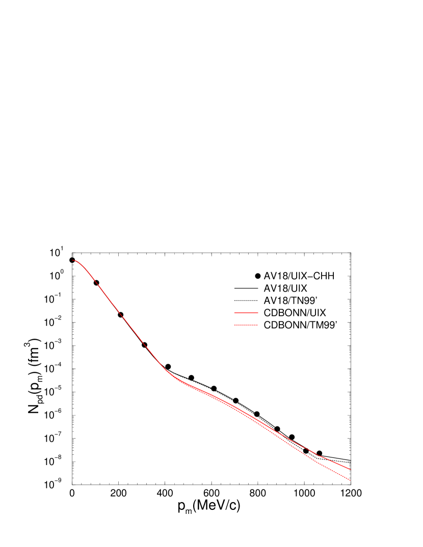
Figure 2: The $p$$d$ momentum distribution, obtained with a correlated-hyperspherical-harmonics (CHH) wave function corresponding to the AV18/UIX Hamiltonian, is compared to those obtained with Faddeev wave functions corresponding to different combinations of two- and three-nucleon interactions.

The $N_{pd}(p_{\rm m})$ momentum distribution, obtained with CHH wave functions corresponding to the AV18/UIX Hamiltonian model, is shown in Fig. 2 up to missing momenta of $\simeq 1$ GeV/c. A number of realistic interactions are currently available, such as, for example, the CD-Bonn Machleidt01 or Nijmegen Stoks94 $N$$N$ and Tucson-Melbourne Coon79 $N$$N$$N$ interactions, and therefore the question arises of how sensitive to the input Hamiltonian are the high momentum components of this momentum distribution. This issue is especially relevant here, since the kinematics of the JLab $(e,e^{\prime}p)$ experiments cover a broad range of $p_{\rm m}$ values, as high as 1.1 GeV/c. It is addressed in Fig. 2, where $p$$d$ momentum distributions, obtained with various combinations of two- and three-nucleon interactions, are compared with each other up to $p_{\rm m}\simeq 1$ GeV/c. All results, but for those labeled AV18/UIX-CHH, are obtained with Faddeev wave functions Nogga04 .

A couple of comments are now in order. First, in the $p_{\rm m}$ range (400–800) MeV/c, there is a significant model dependence: the CD-Bonn $N_{pd}(p_{\rm m})$ is about a factor of 2 smaller than the AV18 one. This is likely a consequence of the fact that the tensor force is weaker in the CD-Bonn than in the AV18. The $p$$d$ overlap in ³He has S- and D-state components, and the associated D-state contribution to $N_{pd}(p_{\rm m})$ indeed becomes dominant at $p_{m}\simeq 400$ MeV/c, it is responsible for the change of slope in $N_{pd}(p_{\rm m})$.

Second, the Faddeev and CHH wave functions corresponding to the AV18/UIX Hamiltonian model lead to $p$$d$ momentum distributions, that are slightly different only in the $p_{\rm m}$ region around 400 MeV/c, where the S-wave contribution changes sign.

V Calculation

Nuclear wave functions, for an assigned spatial configuration ${\bf R}=({\bf r}_{1},\dots,{\bf r}_{A})$, are expanded on a basis of $K$=$2^{A}A!/[Z!(A-Z)!]$ spin-isospin states for $A$ nucleons ($Z$ is the number of protons) as

$$\psi({\bf R})=\sum_{k=1}^{K}\psi_{k}({\bf R})\mid\!k\rangle\ ,$$ (33)

where the components $\psi_{k}({\bf R})$ are generally complex functions of ${\bf R}$, and, in the case $A$=3 and $Z$=2 as an example, the basis states $\mid\!k\rangle$= $\mid\!(n\!\downarrow)_{1}(p\!\downarrow)_{2}(p\!\downarrow)_{3}\rangle$, $\mid\!(n\!\uparrow)_{1}(p\!\downarrow)_{2}(p\!\downarrow)_{3}\rangle$, $\dots\ ,$ $\mid\!(p\!\uparrow)_{1},(p\!\downarrow)_{2}(n\!\downarrow)_{3}\rangle$, $\dots\ .$ Matrix elements of the electromagnetic current operator are written schematically as

$$\langle f\mid O\mid i\rangle=\sum_{k,l=1}^{K}\int{\rm d}{\bf R}\,\psi^{*}_{k}({\bf R};f)O_{kl}({\bf R})\psi_{l}({\bf R};i)\ ,$$ (34)

where $\left[O_{kl}({\bf R})\right]$ denotes the matrix representing in configuration space any of the one- or two-body charge/current operators. Matrix multiplications in the spin-isospin space are performed exactly with the techniques developed in Ref. Schiavilla89 . The problem is reduced to the evaluation of the spatial integrals, which is efficiently carried out with Monte Carlo (MC) methods, although these are implemented differently in the present study than they have been in the past Schiavilla86 ; Schiavilla90 .

To illustrate these methods, consider the PWIA calculation of the one-body charge operator in the process ³He($e,e^{\prime}p$)$d$:

$$\rho^{\rm PWIA}\sim\sum_{k,l}\int{\rm d}{\bf R}\,{\rm e}^{-{\rm i}{\bf p}\cdot{\bf r}_{3}}\,{\rm e}^{-{\rm i}{\bf p}_{f}\cdot{\bf R}_{12}}\,\psi^{*}_{k}({\bf r}_{1}-{\bf r}_{2};f)\,{\rm e}^{{\rm i}{\bf q}\cdot{\bf r}_{3}}\,\rho_{kl}({\bf q};-{\rm i}\nabla_{3})\psi_{l}({\bf R};i)\ ,$$ (35)

where $\psi(i)$ and $\psi(f)$ denote the ³He and $p$+$d$ cluster wave functions, respectively, and $\rho_{kl}({\bf q};-{\rm i}\nabla_{3})$ is $k$$l$ matrix element of the charge operator in Eq. (3). Its dependence on the momentum operator, through the spin-orbit term, has been made explicit. It is convenient to introduce the Jacobi variables, ${\bf x}$=${\bf r}_{3}-{\bf R}_{12}$, ${\bf y}$=${\bf r}_{1}-{\bf r}_{2}$, so that the integral reads

$$\rho^{\rm PWIA}\sim\sum_{k,l}\int{\rm d}{\bf x}{\rm d}{\bf y}\,{\rm e}^{-{\rm i}{\bf p}_{\rm m}\cdot{\bf x}}\,\psi^{*}_{k}({\bf y};f)\rho_{kl}\left({\bf q};-{\rm i}\frac{3}{2}\nabla_{\bf x}\right)\psi_{l}({\bf x},{\bf y};i)\ ,$$ (36)

where ${\bf p}_{\rm m}$ is the missing momentum. In Refs. Schiavilla86 ; Schiavilla90 , this integral was evaluated with the Metropolis algorithm Metropolis53 by sampling the coordinates (${\bf x},{\bf y}$) from a probability density, taken to consist of products of central correlation functions from VMC wave functions (see Ref. Schiavilla86 ). While this procedure is satisfactory at low $p_{\rm m}$, in the sense that statistical errors are small, it becomes impractical as $p_{\rm m}$ increases, due to the rapidly oscillating nature of the integrand. Indeed, this problem is evident in the VMC calculation of the $p$$d$ and $p$$t$ momentum distributions, shown in Ref. Forest96 : even though the random walk consists of a large number (of the order of several hundreds of thousands) of configurations, oscillations in the central values persist at large $p_{\rm m}$ ($>600$ MeV/c).

In the present work, we carry out the multidimensional integrations by a combination of MC and standard quadratures, namely we write

$$\rho^{\rm PWIA}\sim\int{\rm d}{\bf y}\int_{0}^{2\pi}{\rm d}\phi_{x}W(\phi_{x},{\bf y})\,F(\phi_{x},{\bf y})\simeq\frac{1}{N_{c}}\sum_{c=1}^{N_{c}}F(c)\ ,$$ (37)

where the $c$’s denote configurations $(\phi_{x},{\bf y})$ (total number $N_{c}$), sampled with the Metropolis algorithm from a probability density $W$ (normalized to one), given by

$$W(\phi_{x},{\bf y})=\frac{1}{2\pi}\sum_{k}|\psi_{k}({\bf y};f)|^{2}\ .$$ (38)

Note that $W$ is uniform in $0\leq\phi_{x}\leq 2\pi$. For each configuration $c$, the function $F$ is obtained by Gaussian integrations over the $x$ and ${\rm cos}\,\theta_{x}$ variables, i.e.

$$F(c)=\frac{1}{W(c)}\sum_{k,l}\int_{-1}^{1}{\rm d}({\rm cos}\theta_{x})\int_{0}^{\infty}{\rm d}x\,x^{2}\,{\rm e}^{-{\rm i}{\bf p}_{\rm m}\cdot{\bf x}}\,\psi^{*}_{k}({\bf y};f)\rho_{kl}\left({\bf q};-{\rm i}\frac{3}{2}\nabla_{\bf x}\right)\psi_{l}({\bf x},{\bf y};i)\ .$$ (39)

As a result, the statistical errors are very significantly reduced. In Fig. 2 the CHH calculation of $N_{pd}(p_{\rm m})$ is carried out with this method, it uses a random walk consisting only of 20,000 configurations. However, convergence in the ($x$,${\rm cos}\,\theta_{x}$) integrations requires of the order of (70,50) Gaussian points at the highest $p_{\rm m}$, and so the present method turns out to be computationally more time-consuming than the earlier version at high $p_{\rm m}$.

Additional refinements in the present MC implementation are i) the application of gradient operators on the left, rather than right, wave function, and ii) the use of block averaging for a more realistic estimation of the statistical errors.

Gradient operators, such as those occurring in the one-body electromagnetic current, are discretized as

$$\nabla_{i,\alpha}\psi({\bf R})\simeq\frac{\psi(\dots{\bf r}_{i}+\delta\,\hat{\bf e}_{\alpha}\dots)-\psi(\dots{\bf r}_{i}-\delta\,\hat{\bf e}_{\alpha}\dots)}{2\,\delta}\ ,$$ (40)

where $\delta$ is a small increment ($\delta$=0.0005 fm in the calculations reported here) and $\hat{\bf e}_{\alpha}$ is a unit vector in the $\alpha$-direction. Therefore, again in the context of the PWIA calculation above, the $\nabla_{\bf x}\ ,$ when operating on the left, only acts on the plane wave—in fact, an eigenfunction of $\nabla_{\bf x}\ .$ This further reduces statistical errors, and also ensures that the PWIA relations in Eq. (29) are satisfied—modulo tiny discretization errors of order $(\delta\,p_{\rm m})^{2}$—at each configuration in the random walk, which would not be the case if the gradient were left to operate on the ³He wave function to the right. Of course, the eigenfunction property above is spoiled, when final state interactions are taken into account; however, the error-reduction benefits remain. The disadvantage of the procedure just outlined is that it leads to an increase in computational time, since the various gradients have to be evaluated, rather than once (when acting to the right), as many times as the number of kinematics being considered in the calculation.

A crude estimate of the MC error is obtained as

$$\Delta(F)=\frac{1}{\sqrt{N_{c}}}\left[\frac{1}{N_{c}}\sum_{c=1}^{N_{c}}F^{\,2}(c)-\left[\frac{1}{N_{c}}\sum_{c=1}^{N_{c}}F(c)\right]^{\!2}\,\right]^{1/2}\ ,$$ (41)

it assumes that the distribution $F(c)$ is Gaussian, whereas in practice this is generally not the case. A better estimate, adopted in the present work, is obtained by dividing the set of $N_{c}$ samples into $M_{c}$ blocks containing $n_{c}$ samples each:

$$f_{m}=\frac{1}{n_{c}}\sum_{c=(m-1)\,n_{c}+1}^{m\,n_{c}}F(c)\ .$$ (42)

Then,

$$\Delta(f)=\frac{1}{\sqrt{M_{c}}}\left[\frac{1}{M_{c}}\sum_{m=1}^{M_{c}}f^{\,2}_{m}-\left(\frac{1}{M_{c}}\sum_{m=1}^{M_{c}}f_{m}\right)^{\!2}\,\right]^{1/2}\ ,$$ (43)

where $n_{c}$ can be chosen large enough so as to make the distribution of $f_{m}$ Gaussian (in practice, $n_{c}$ has been taken of the order of 100).

VI Results

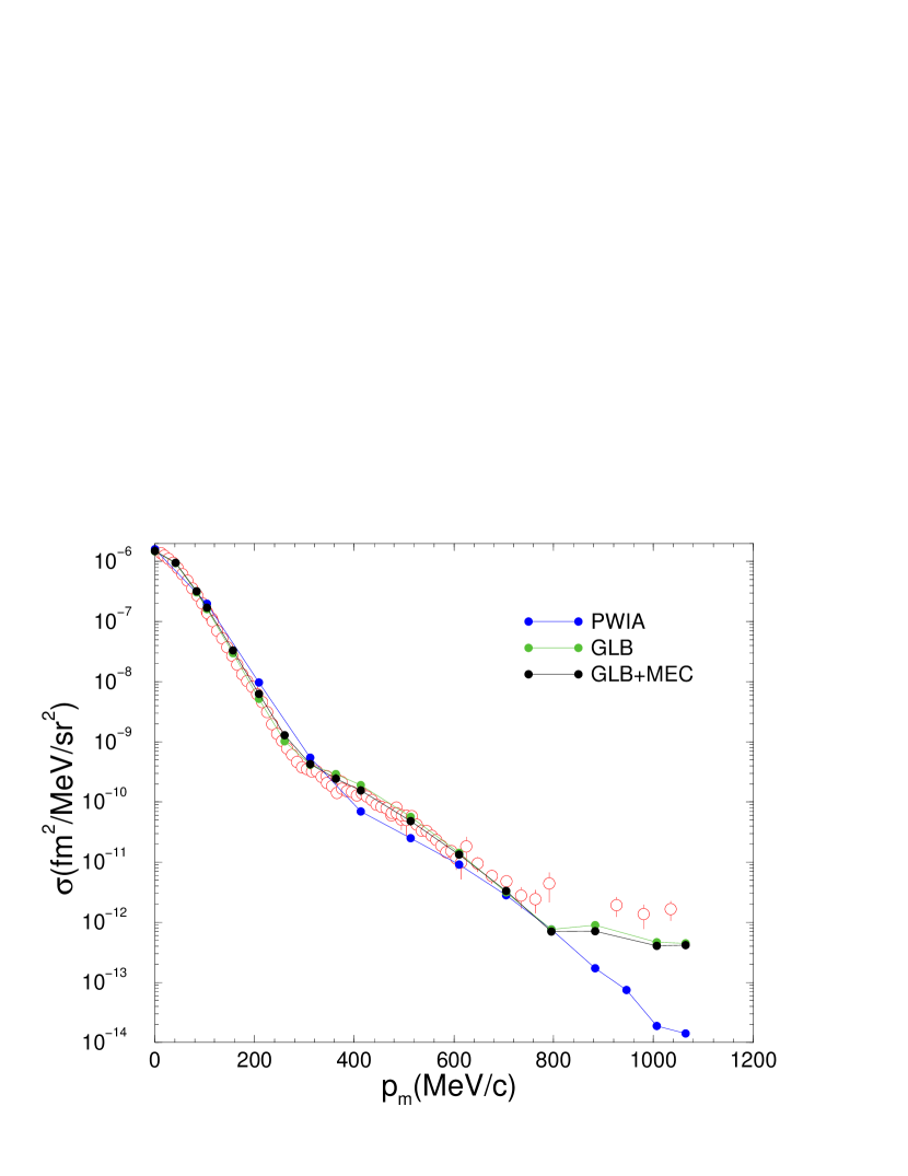
Figure 3: The experimental data for the ³He$(e,e^{\prime}p)$$d$ cross section at $\phi$=180 deg are compared to the results of calculations in plane-wave-impulse-approximation (PWIA), or using the Glauber approximation without (GLB) and with (GLB+MEC) inclusion of two-body currents. The profile operator in the Glauber expansion is derived from the full $N$$N$ scattering amplitude, boosted from the c.m. to the the rescattering (i.e., lab) frame.

The predicted cross sections are compared with the data taken at JLab (E89-044) Rvachev05 in Figs. 3 and 4. The in-plane measurements were carried out in quasi-elastic kinematics with the proton being detected on either side of the three-momentum transfer ${\bf q}$ (the kinematics in Figs. 3 and  4 have, respectively, $\phi$=180 deg and 0 deg, in the notation of Sec. IV). From these cross sections, the longitudinal-transverse asymmetry $A_{LT}$ is obtained as

$$A_{LT} = \frac{\sigma(\phi=0\,{\rm deg})-\sigma(\phi=180\,{\rm deg})}{\sigma(\phi=0\,{\rm deg})+\sigma(\phi=180\,{\rm deg})}$$ (44)

$$= \frac{v_{LT}\,R_{LT}}{v_{L}\,R_{L}+v_{T}\,R_{T}+v_{TT}\,R_{TT}}\ ,$$

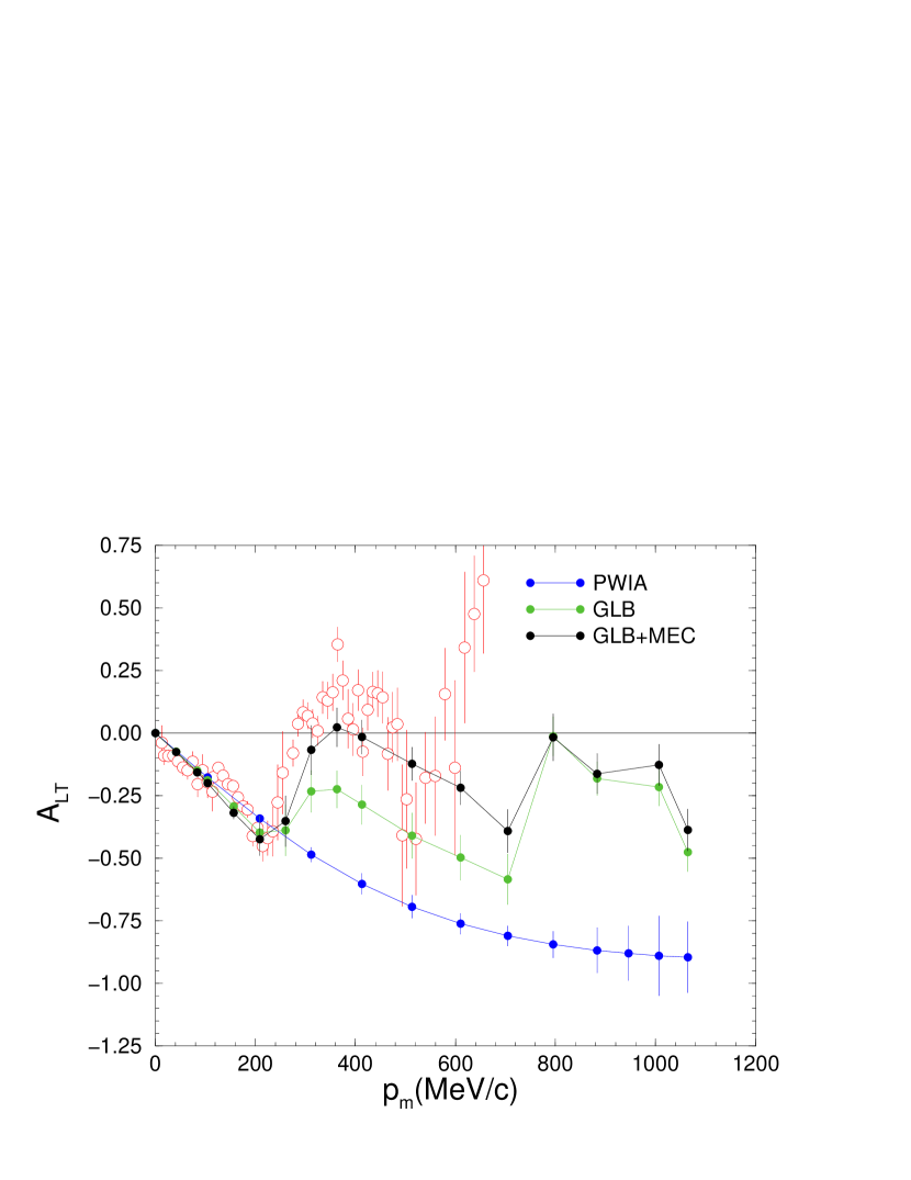
Figure 5: Same as in Fig. 3, but for the longitudinal-transverse asymmetry rather than the cross section.

where $\sigma(\phi)$ stands for the five-fold differential cross section in Eq. (23). Thus, the asymmetry, shown in Fig. 5, is proportional to the $R_{LT}$ response function. Note that $v_{LT}$ is negative, as defined in Ref. Raskin89 .

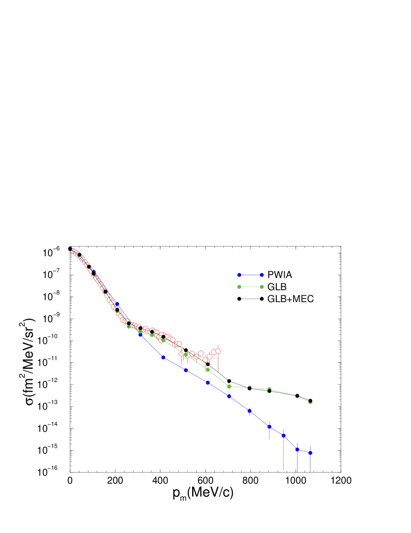
Figure 4: Same as in Fig. 3, but at $\phi$=0 deg.

In the figures, the results of three different calculations are displayed. The curve labeled PWIA is a plane-wave-impulse-approximation calculation, based on the CHH ³He wave function corresponding to the AV18/UIX Hamiltonian model (the resulting $p$$d$ momentum distribution is shown in Fig. 2). It neglects final-state-interaction (FSI) effects and contributions from two-body currents (MEC). The present PWIA results are in agreement with those of recent studies Ciofi05a ; Laget05 : they overpredict the measured cross section for values of the missing momentum $p_{\rm m}$ up to $\simeq 300$ MeV/c, while underpredicting it at high $p_{\rm m}$. This underprediction is particularly severe for the kinematics with $\phi$=0 deg (Fig. 4): the contribution proportional to $R_{LT}$ in Eq. (23) is comparable in magnitude for $p_{\rm m}>300$ MeV/c, but of opposite sign, relative to that from $R_{L}$ and $R_{T}$ (the $R_{TT}$ contribution is negligible). Of course, when $\phi$=180 deg, they have the same sign.

The curve labeled GLB (GLB+MEC) shows the results of calculations using the Glauber approximation to describe FSI and one-body (one- plus two-body) currents. Both single- and double-rescattering terms are retained in the Glauber treatment of the final $p$+$d$ scattering state. The profile operator is obtained from the full $N$$N$ scattering amplitude, boosted from the c.m. to the rescattering frame as discussed in Sec. III.3. The invariant energy $\sqrt{s}$ at which the rescattering process occurs, Eq. (11), changes little over the whole range of missing momenta, it corresponds to a lab kinetic energy of $\simeq$ 830 MeV. Thus the parameters used for the central, single and double spin-flip terms of the $p$$p$ and $p$$n$ amplitudes are taken from the last row of, respectively, Tables III and IV of Ref. Wallace81 . However, the parameters for the $B^{pn}(k)$ and $E^{pn}(k)$ terms (in the notation of Ref. Wallace81 ), corresponding to $m$=2 and 5 in Eq. (15), are replaced by those for $B^{pp}(k)$ and $E^{pp}(k)$, since the real parts of $\beta_{B}^{pn}$ and $\beta_{E}^{pn}$ are negative.

There is satisfactory agreement between theory and experiment up to missing momenta of 700 MeV/c. At values of $p_{\rm m}\simeq 1$ GeV/c, however, the theoretical results are smaller than the experimental values by about a factor of two, although they do reproduce the flattening of the cross section, as function of $p_{\rm m}$, seen in the data. Final-state-interaction effects play a crucial role: they reduce the PWIA cross section at low $p_{\rm m}$ ($<300$ MeV/c), and increase it very substantially at larger values of $p_{\rm m}$. Two-body current contributions, while not large, are not negligible, and improve the agreement between theory and experiment. This is most clearly illustrated in the case of the $A_{LT}$ observable, Fig. 5.

It would be interesting to investigate the model dependence due to the input Hamiltonian used to generate the bound-state wave functions. We do not expect it to be large, even for $p_{\rm m}=(400$–800) MeV/c where the calculated $p$$d$ momentum distributions can differ by as much as a factor of two, see Fig. 2. The cross section in this range of $p_{\rm m}$ values results from strength shifted by FSI from the low $p_{\rm m}$ region, $p_{\rm m}$ up to $\simeq 300$ MeV/c, where the $N_{pd}(p_{\rm m})$ model dependence is negligible. Clearly, a direct calculation is needed to verify whether this expectation is justified.

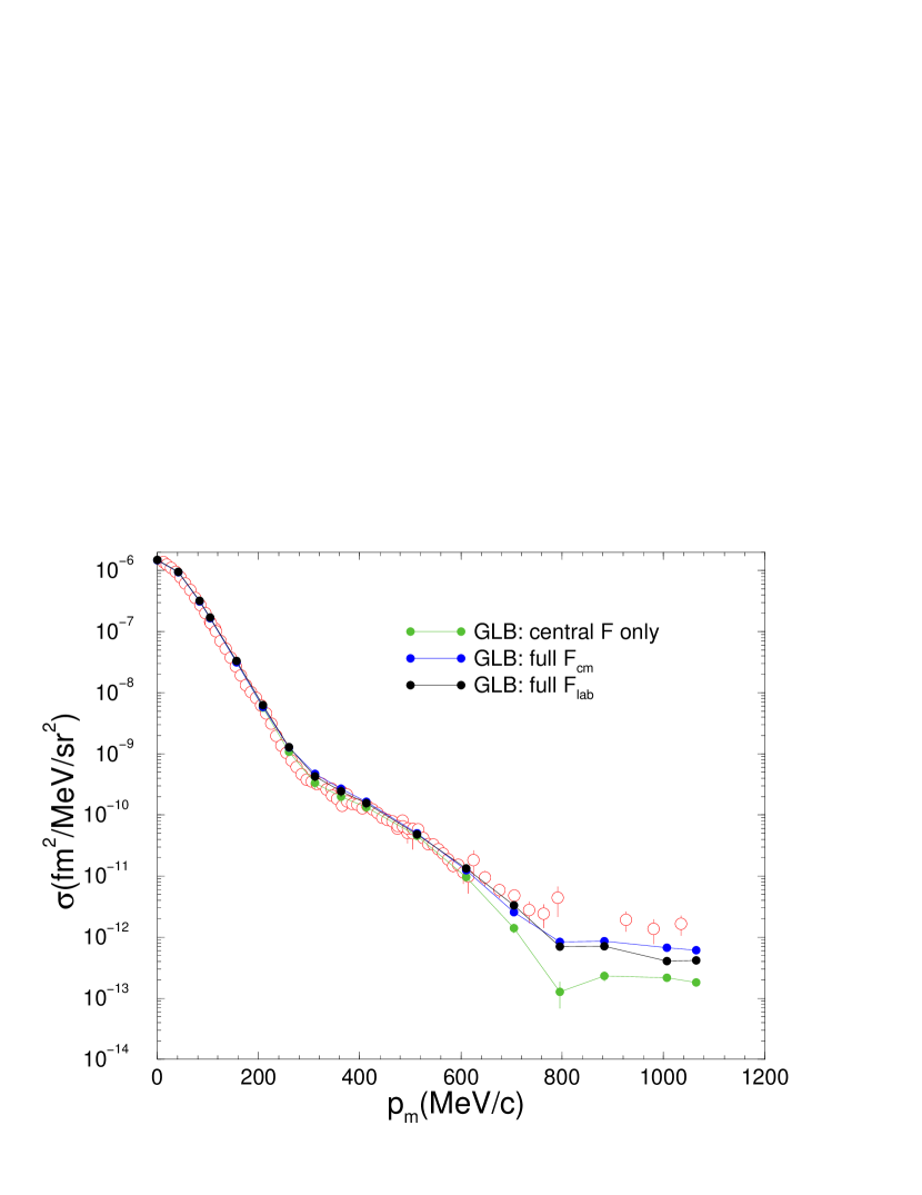
Figure 6: The experimental data for the ³He$(e,e^{\prime}p)$$d$ cross section at $\phi$=180 deg are compared to results of Glauber calculations, using a variety of approximation schemes for the $N$$N$ scattering amplitude. See text for an explanation of the notation.

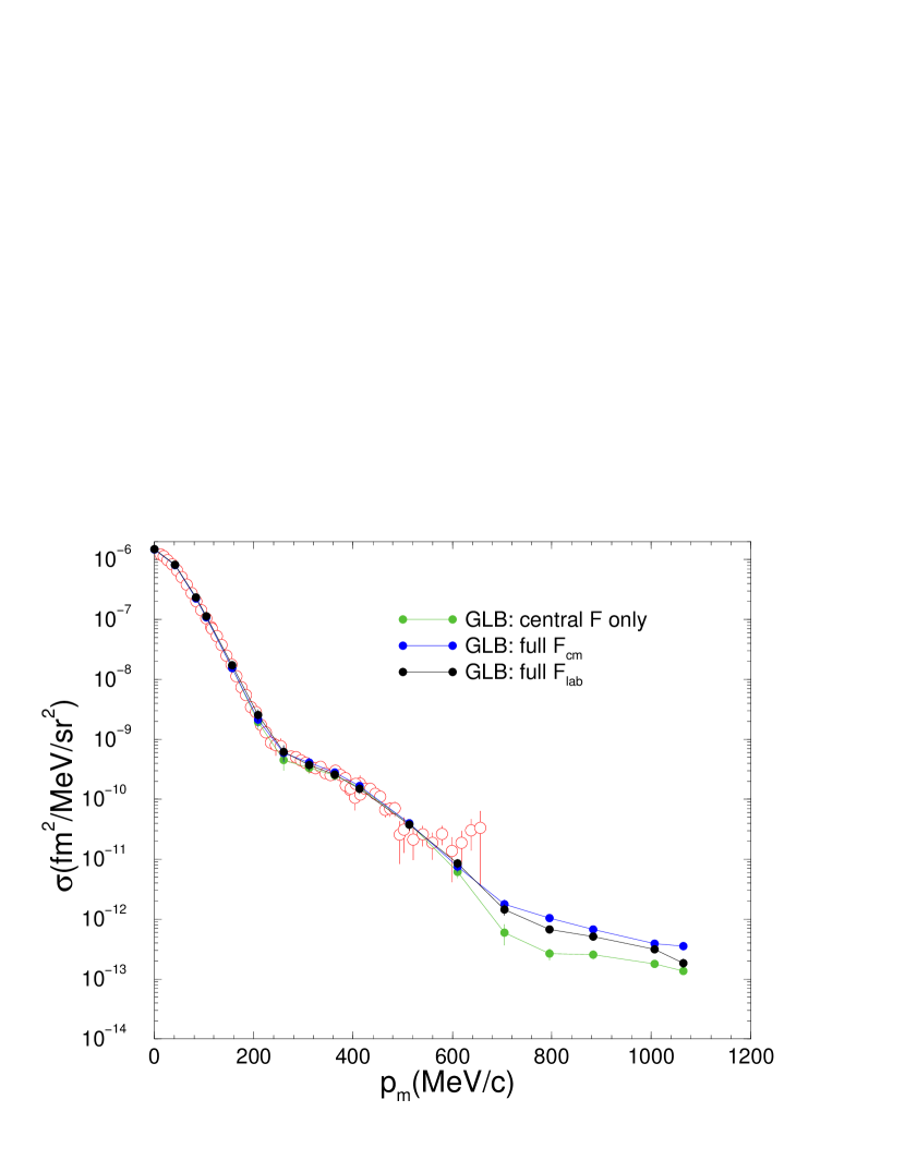
Figure 7: Same as in Fig. 6, but at $\phi$=0 deg.

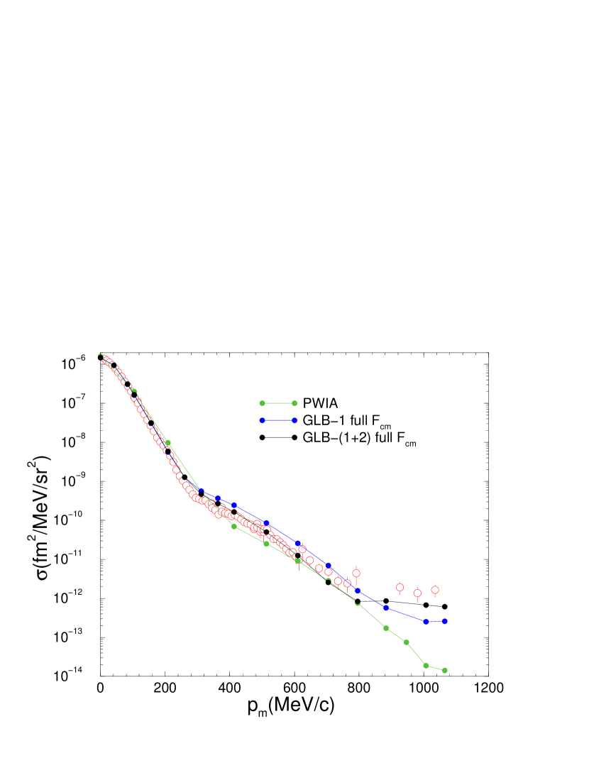
Figure 8: The experimental data for the ³He$(e,e^{\prime}p)$$d$ cross section at $\phi$=180 deg are compared to Glauber calculations including only single (GLB-1) or both single and double [GLB(1+2)] rescattering terms. Boost corrections in the $N$$N$ scattering amplitude are neglected. Note that two-body current contributions are included.

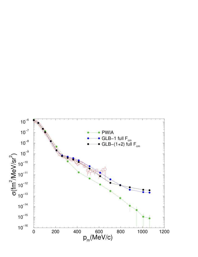
Figure 9: Same as in Fig. 8, but at $\phi$=0 deg.

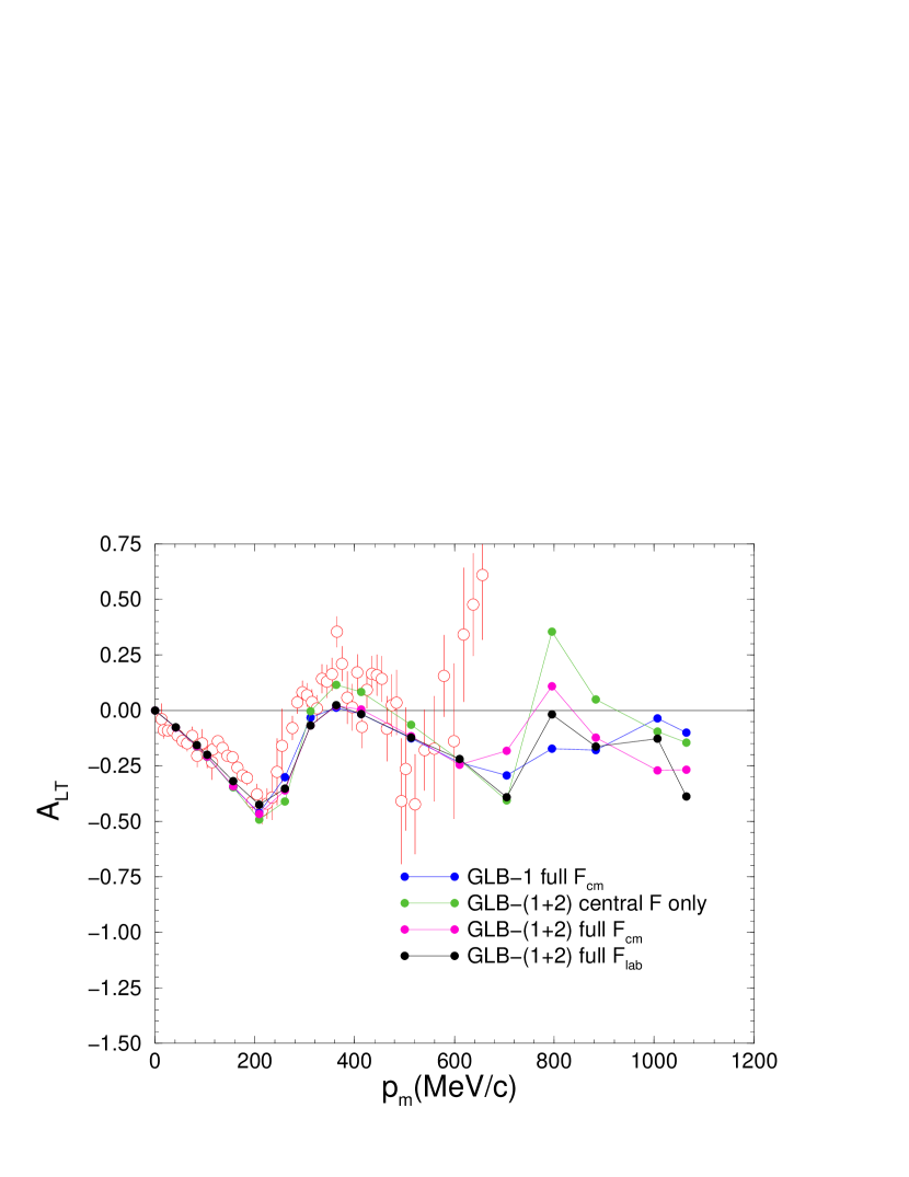
Figure 10: The experimental data for the longitudinal-transverse asymmetry in the ³He$(e,e^{\prime}p)$$d$ reaction are compared to the results of Glauber calculations including only single (GLB-1) or both single and double [GLB-(1+2)] rescattering terms. The GLB-(1+2) calculations use the full $N$$N$ scattering amplitude, with (full $F_{\rm lab}$) or without (full $F_{\rm cm}$) boost corrections, or its central term only (central $F$ only). The GLB-1 calculation uses the full $N$$N$ scattering amplitude, but ignores boost effects. Note that two-body current contributions are included in all calculations.

The next set of figures, Figs. 6–10, is meant to illustrate the effect of various approximation schemes in the Glauber treatment of FSI. In all calculations MEC contributions are included. In Figs. 6 and 7 the results of calculations using i) only the central part of the scattering amplitude (curves labeled “central F only”) and ii) the full scattering amplitude but neglecting boost corrections (curves labeled “full F_cm”) are compared with the baseline GLB+MEC results of Figs. 3 and 4 (labeled here as “full F_lab”). For values of $p_{\rm m}>600$ MeV/c, the spin-dependence of the $N$$N$ scattering amplitude, which is ignored in all Glauber calculations of $(e,e^{\prime}p)$ reactions off few-body nuclei we are aware of (see, for example, Refs. Benhar00 ; Ryckebusch03 ; Ciofi05 ; Ciofi05a ), leads to a very substantial increase of the cross section obtained when using the central term only. On the other hand, boost corrections, which in the present work are only accounted for approximately (see Sec. III.3), seem to be small, although not negligible.

In Figs. 8 and 9, the results of calculations using the full scattering amplitude in the c.m. frame but including only single rescattering in the Glauber expansion (curve labeled “GLB-1 full F_cm”), i.e. the term $G^{(1)}$ of Eq. (8), are compared with the predictions obtained by retaining both single and double rescatterings (the curve labeled “GLB-(1+2) full F_cm”is the same as “full F_cm”in the previous two figures). Also shown are the PWIA results. At low missing momenta (below 300 MeV/c) interference between the plane-wave and single-rescattering amplitudes reduces the PWIA cross section. In the $p_{\rm m}$ range $\simeq(300-800)$ MeV/c destructive interference occurs between the leading single- and double-rescattering amplitudes, resulting in a reduction of the cross section obtained in the GLB-1 calculation. At the highest values of $p_{\rm m}$, double-rescattering processes are dominant. The interference pattern among these various amplitudes is consistent with that obtained in the calculations of Ref. Ciofi05a .

Lastly, the $A_{LT}$ asymmetry is found to be relatively insensitive to the various approximation schemes discussed above in the region where measurements are available ($p_{\rm m}<600$ MeV/c). All calculations reproduce quite well the oscillating behavior of the $A_{LT}$ data.

As already mentioned, most Glauber calculations of $A(e,e^{\prime}p)$ reactions have only used the central part of the $N$$N$ scattering amplitude $F_{ij}^{NN}$, i.e.

$$(2{\rm i}\,p)^{-1}\,F^{NN}_{ij}({\bf k},s)\longrightarrow\frac{1}{8\pi}\sigma^{NN}(s)\left[1-{\rm i}\rho^{NN}(s)\right]\,{\rm exp}\left[-\beta^{NN}(s){\bf k}^{2}\right]\ ,$$ (45)

where $\sigma^{NN}(s)$ and $\rho^{NN}(s)$ are, respectively, the total cross section and ratio of the real to imaginary part of the scattering amplitude at the invariant energy $\sqrt{s}$. While the values for $\sigma^{NN}(s)$ and, to a less extent, $\rho^{NN}(s)$ are well known for both $p$$p$ and $p$$n$ over a wide range of $\sqrt{s}$ (see, for example, Ref. Ryckebusch03 and references therein), this is not the case for $\beta^{NN}(s)$. This parameter is determined by fitting either the elastic differential cross section at forward scattering angles (as in Ref. Ryckebusch03 and references therein), i.e. ${\rm d}\sigma^{NN}_{\rm el}(s,t)/{\rm d}t$ for small four-momentum transfer $t$, or rather the central term of the scattering amplitude derived from phase-shift analyses (as in Ref. Wallace81 and references therein). It should be emphasized that the first procedure tacitly assumes that the contributions to ${\rm d}\sigma^{NN}_{\rm el}(s,t)/{\rm d}t$ due to spin-dependent terms in $F_{ij}^{NN}$ are negligible. It is not obvious that this assumption is justified. For example, large cross section differences, $\Delta\sigma_{L}^{NN}$, between spin orientations parallel and antiparallel to the beam direction are observed in $p$$p$ and $p$$n$ scattering Lechanoine93 . Also observed are substantial, although less dramatic, cross section differences, $\Delta\sigma_{T}^{NN}$, between parallel and antiparallel transverse spin orientations Lechanoine93 .

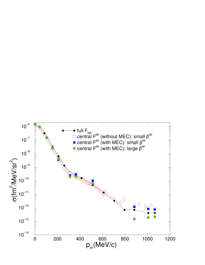
Figure 11: The experimental data for the ³He$(e,e^{\prime}p)$$d$ cross section at $\phi$=180 deg are compared to results of Glauber calculations using the full $N$$N$ scattering amplitude (curve labeled “full $F_{\rm lab}$”), or its central term only with a $\beta^{pp}$ parameter consistent with either ${\rm d}\sigma_{\rm el}^{pp}/{\rm d}t$ at small $t$ (curve labeled “central $F^{pp}$: small $\beta^{pp}$”) or phase-shift analyses (curve labeled “central $F^{pp}$: large $\beta^{pp}$”). All curves include two-body current contributions. For the “central $F^{pp}$: small $\beta^{pp}$”calculation also shown are the results obtained with one-body currents.

The sensitivity of the ³He($e,e^{\prime}p$)$d$ cross section, calculated using these two different values for the $\beta^{pp}$ parameter (the isospin dependence is ignored in the following discussion), is illustrated in Figs. 11 and 12. The curves labeled “central F^pp: small $\beta^{pp}$”was obtained with $\beta^{pp}$= 0.095 fm², as reported in Ref. Ryckebusch03 (for $pp$ scattering). The curve labeled “central F^pp: large $\beta^{pp}$”was obtained, instead, with $\beta^{pp}$=0.157 fm², a value in line with that inferred from phase-shift analyses Wallace81 . Incidentally, this large $\beta^{pp}$ was used in a set of unpublished calculations carried out by the present authors in 2004 (and referred to in Refs. Rvachev05 ; Ciofi05a ; Laget05 ).

The results of the calculation with a small $\beta^{pp}$, including only one-body currents, are in quantitative agreement with those of Ref. Ciofi05a , although at $p_{\rm m}\simeq 400-700$ MeV/c the present predictions are somewhat larger than obtained in Ref. Ciofi05a . These relatively small differences are presumably due to i) the breakdown of the factorization approximation employed in Ref. Ciofi05a , and ii) the use of the CC1 parameterization deForest83 adopted in Ref. Ciofi05a , rather than free nucleon form factors as in the present study.

In the high $p_{\rm m}$ ($\simeq 1$ GeV/c) the small $\beta^{NN}$ results lead to a large increase of FSI contributions. The profile function corresponding to a central scattering amplitude reads

$$\Gamma^{NN}({\bf b};s)=\frac{1}{8\pi\,\beta^{NN}(s)}\sigma^{NN}(s)\left[1-{\rm i}\rho^{NN}(s)\right]\,{\rm exp}\left[-\frac{{\bf b}^{2}}{4\beta^{NN}(s)}\right]\ ,$$ (46)

and a small $\beta^{NN}$, while reducing its range, makes the value at zero impact parameter larger, which leads to the FSI enhancement mentioned above.

Lastly, it is interesting to note that the results of the calculation based on the full scattering amplitude derived from phase-shift analyses are close to those using the central term only in the amplitude with a $\beta^{NN}$ parameter obtained from the small $t$ slope of the elastic cross section.

VII Conclusions

In this work we carried out calculations of the ³He$(e,e^{\prime}p)$$d$ cross section for the kinematics of JLab experiment E89-044, spanning the missing momentum range (0–1.1) GeV/c. Final state interactions were treated in the Glauber approximation, including both single and double rescattering terms. In contrast to earlier studies of the same process Laget05 ; Ciofi05a , the profile operator retained the full spin and isospin dependence of the underlying $N$$N$ scattering amplitudes. Parameterizations for these were derived from phase-shift analyses in Ref. Wallace81 . It would be desirable to update and improve these parameterizations, although the paucity of additional $N$$N$ scattering data at energies beyond 500 MeV collected in the last two decades or so (due in part to the termination of $N$$N$ programs at facilities such as Saturne and LAMPF) will presumably not alter them significantly.

Corrections arising from boosting the amplitude from the c.m. to the relevant frame for the rescattering processes were found to be relatively small. However, the boosting procedure was only implemented approximately.

Theory and experiment are in quantitative agreement for missing momenta in the range (0–700) MeV/c. Rescattering effects play a crucial role over the whole range of $p_{\rm m}$, in particular double rescattering processes are responsible for the increase of the cross section at $p_{\rm m}\simeq 1$ GeV/c, which, nevertheless, is still underpredicted by theory by about a factor of two. However, the flattening of the data in this $p_{\rm m}$ region is well reproduced. Two-body current contributions are relatively small, but helpful in bringing theoretical predictions for the $A_{LT}$ observable in significantly better agreement with experiment. Spin-dependent terms in the scattering amplitude are important at high $p_{\rm m}$.

A generalized Glauber approach has been recently developed for $(e,e^{\prime}p)$ processes Frankfurt97 ; Sargsian05 which attempts to partially remove the frozen approximation implicit in the original derivation Glauber59 . The resulting correction leads, in essence, to a modification of the profile operator by a phase factor $\Gamma_{ij}\longrightarrow{\rm exp}({\rm i}\Delta_{0}z_{ij})\,\Gamma_{ij}$, with $\Delta_{0}$ fixed by the kinematics, $\Delta_{0}=\omega\,E_{\rm m}/q$. It was found to be numerically very small, at the most 10% at $p_{\rm m}\simeq 1$ Gev/c. It may play a more prominent role, however, in the three-body electrodisintegration ³He$(e,e^{\prime}p)$$p$$n$ at high missing energies.

Glauber calculations using only the central part of the scattering amplitude with a $\beta^{NN}$ obtained by fitting the low $t$ slope of ${\rm d}\sigma_{\rm el}^{NN}/{\rm d}t$ are close to those using the full amplitude derived from phase-shift analyses. As argued in the previous section, however, it is not clear that one is justified in ignoring the spin dependence of the amplitude in view of the large cross section differences observed in $N$$N$ scattering involving polarized beam and target (see, for example, Ref. Lechanoine93 ).

Future work aims at: i) extending the present Glauber approximation, based on a spin- and isospin-dependent scattering amplitude, to treat the $p$+³H electrodisintegration of ⁴He and, in particular, the reaction ⁴He$(\vec{e},e^{\prime}{\vec{p}}\,)$³H, both of which have been recently measured at JLab Strauch03 ; Reitz05 (the polarization parameters measured in the ⁴He$(\vec{e},e^{\prime}{\vec{p}}\,)$³H reaction Strauch03 have already been found to be in agreement with the results of a calculation using an optical potential Schiavilla05a ); ii) investigating the model dependence of the present predictions for the ³He$(e,e^{\prime}p)$$d$ cross section upon the input (non-relativistic) Hamiltonian adopted to generate the bound-state wave functions; iii) exploring the extent to which the use of a relativistic Hamiltonian Carlson93 to generate these wave functions alters the present predictions, particularly at high $p_{\rm m}$ (the research projects in items ii) and iii) will be made possible by very recent developments of the hyperspherical-harmonics method in momentum space Kievsky05 ); and iv) applying the methods developed here to the three-body electrodisintegration of ³He. Studies along these lines are being vigorously pursued.

Appendix A

We list here explicit expressions for the single-proton response functions $r^{p}_{\alpha}$ defined in Eq. (29):

$$r_{L}^{p} = \left(\frac{q}{Q}\right)^{2}\left[G_{Ep}^{2}+\frac{\eta}{1+\eta}\left(\frac{p_{\perp}}{m}\right)^{2}\left(G_{Mp}-\frac{1}{2}G_{Ep}\right)^{2}\right]\ ,$$

$$r_{T}^{p} = \left(\frac{Q}{q}\right)^{2}\left[\frac{q^{2}}{2m^{2}}G_{Mp}^{2}+\left(\frac{p_{\perp}}{m}\right)^{2}\left[\left(G_{Ep}+\frac{\eta}{2}G_{Mp}\right)^{2}+\left(\frac{\omega}{4m}\right)^{2}G_{Mp}^{2}\right]\right]\ ,$$

$$r_{LT}^{p} = 2\sqrt{2}\,\left(\frac{p_{\perp}}{m}\right)\left[G_{Ep}\left(G_{Ep}+\frac{\eta}{2}G_{Mp}\right)+\frac{q}{Q}\frac{\eta}{\sqrt{1+\eta}}G_{Mp}\left(G_{Mp}-\frac{1}{2}G_{Ep}\right)\right]\ ,$$

$$r_{TT}^{p} = -\left(\frac{Q}{q}\right)^{2}\left(\frac{p_{\perp}}{m}\right)^{2}\left[\left(G_{Ep}+\frac{\eta}{2}G_{Mp}\right)^{2}-\left(\frac{\omega}{4m}\right)^{2}G_{Mp}^{2}\right]\ ,$$

where $p_{\perp}$ is (the magnitude of) the component of the proton momentum transverse to the momentum transfer ${\bf q}$, and $\eta$=$Q^{2}/(4m^{2})$. The dependence of the proton electric ($G_{Ep}$) and magnetic ($G_{Mp}$) form factors on $Q^{2}$ is understood.

Figure 1: Schematic illustration of single, panel a), and double, panel b), rescattering processes. Dashed (solid) lines represent virtual photons (nucleons), while black solid circles represent $N$$N$ scattering amplitudes.

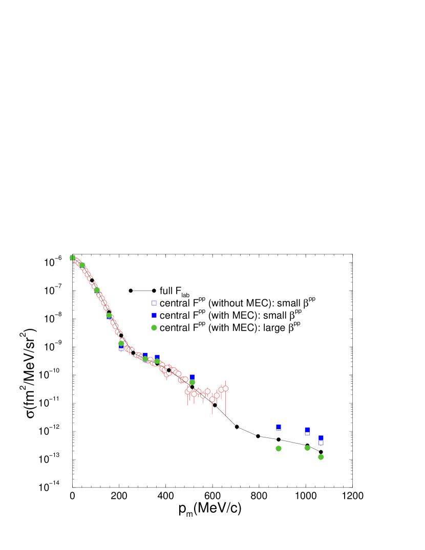
Figure 12: Same as in Fig. 11, but at $\phi$=0 deg.

References

- (1) M.M. Rvachev et al., Phys. Rev. Lett. 94, 192302 (2005).
- (2) F. Benmokhtar et al., Phys. Rev. Lett. 94, 082305 (2005).
- (3) C. Ciofi degli Atti and L.P. Kaptari, Phys. Rev. C 71, 024005 (2005).
- (4) C. Ciofi degli Atti and L.P. Kaptari, Phys. Rev. Lett. 95, 052502 (2005).
- (5) J.-M. Laget, nucl-th/0410003 and Phys. Rev. C in press.
- (6) J.-M. Laget, Phys. Lett. B609, 49 (2005).
- (7) S. Strauch et al., Phys. Rev. Lett. 91, 052301 (2003).
- (8) P. Lava, J. Ryckebusch, V. Van Overmeire, and S. Strauch, Phys. Rev. C 71, 014605 (2005).
- (9) R.B. Wiringa, V.G.J. Stoks, and R. Schiavilla, Phys. Rev. C 51, 38 (1995).
- (10) B.S. Pudliner, V.R. Pandharipande, J. Carlson, and R.B. Wiringa, Phys. Rev. Lett. 74, 4396 (1995).
- (11) A. Kievsky, M. Viviani, and S. Rosati, Nucl. Phys. A551, 241 (1993); A. Kievsky, Nucl. Phys. A624, 125 (1997).
- (12) A. Nogga et al., Phys. Rev. C 67, 034004 (2003).
- (13) L.E. Marcucci, D.O. Riska, and R. Schiavilla, Phys. Rev. C 58, 3069 (1998).
- (14) J. Carlson and R. Schiavilla, Rev. Mod. Phys. 70, 743 (1998).
- (15) L.E. Marcucci, K.M. Nollett, R. Schiavilla, and R.B. Wiringa, nucl-th/0402078 and Nucl. Phys. A in press.
- (16) J. Carlson, J. Jourdan, R. Schiavilla, and I. Sick, Phys. Rev. C 65, 024002 (2000).
- (17) S. Jeschonnek and T.W. Donnelly, Phys. Rev. C 57, 2438 (1998).
- (18) G. Höhler et al., Nucl. Phys. B114, 505 (1976).
- (19) L.E. Marcucci, M. Viviani, R. Schiavilla, A. Kievsky, and S. Rosati, Phys. Rev. C 72, 014001 (2005).
- (20) C. Lechanoine-Leluc and F. Lehar, Rev. Mod. Phys. 65, 47 (1993).
- (21) R.J. Glauber, Lectures in Theoretical Physics, edited by W. Brittain and L.G. Dunham (Interscience, New York, 1959), Vol. 1.
- (22) S.J. Wallace, in Advances in Nuclear Physics, edited by J. Negele and E. Vogt (Plenum, New York, 1981), Vol. 12, p. 135.
- (23) O. Benhar, N.N. Nikolaev, J. Speth, A.A. Usmani, and B.G. Zakharov, Nucl. Phys. A673, 241 (2000).
- (24) R. Arndt, L.D. Roper, R.A. Bryan, R.B. Clark, B.J. VerWest, and P. Signell, Virginia Polytechnic Institute and State University Report VPISA-2(82), 1982.
- (25) J. Ryckebusch, D. Debruyne, P. Lava, S. Janssen, B. Van Overmeire, and T. Van Cauteren, Nucl. Phys. A 728, 226 (2003).
- (26) J.A. McNeil, L. Ray, and S.J. Wallace, Phys. Rev. C 27, 2123 (1983).
- (27) A.S. Raskin and T.W. Donnelly, Ann. Phys. 191, 78 (1989).
- (28) R. Schiavilla, V.R. Pandharipande, and R.B. Wiringa, Nucl. Phys. A449, 219 (1986).
- (29) J.L. Forest, V.R. Pandharipande, S.C. Pieper, R.B. Wiringa, R. Schiavilla, and A. Arriaga, Phys. Rev. C 54, 646 (1996); R.B. Wiringa, private communication.
- (30) R. Schiavilla, O. Benhar, A. Kievsky, L.E. Marcucci, and M. Viviani, to be published.
- (31) R. Machleidt, Phys. Rev. C 63, 024001 (2001).
- (32) V.G.J. Stoks, R.A.M. Klomp, C.P.F. Terheggen, and J.J. de Swart, Phys. Rev. C 49, 2950 (1994).
- (33) S.A. Coon, M.D. Scadron, P.C. McNamee, B.R. Barrett, D.W.E. Blatt, and B.H.J. McKellar, Nucl. Phys. A317, 242 (1979); S.A. Coon and H.K. Han, Few-Body Syst. 30, 131 (2001).
- (34) A. Nogga and W. Glöckle, private communication; H. Witala, A. Nogga, H. Kamada, W. Glöckle, J. Golak, and R. Skibiński, Phys. Rev. C 68, 034002 (2003).
- (35) R. Schiavilla, V.R. Pandharipande, and D.O. Riska, Phys. Rev. C 40, 2294 (1989).
- (36) R. Schiavilla, Phys. Rev. Lett. 65, 835 (1990).
- (37) N. Metropolis, A.W. Rosenbluth, M.N. Rosenbluth, A.H. Teller, and E. Teller, J. Chem. Phys. 21, 1087 (1953).
- (38) T. de Forest, Nucl. Phys. A392, 232 (1983).
- (39) L.L. Frankfurt, M.M. Sargsian, and M.I. Strikman, Phys. Rev. C 56, 1124 (1997).
- (40) M.M. Sargsian, T.V. Abrahamyan, M.I. Strikman, and L.L. Frankfurt, Phys. Rev. C 71, 044614 (2005).
- (41) B. Reitz, for the Jefferson Lab Hall A Collaboration, Perspectives in Hadronic Physics, S. Boffi, C. Ciofi degli Atti, and M.M. Giannini, Eds., Springer, 2004, p. 165.
- (42) R. Schiavilla, O. Benhar, A. Kievsky, L.E. Marcucci, and M. Viviani, Phys. Rev. Lett. 94, 072303 (2005).
- (43) J. Carlson, V.R. Pandharipande, and R. Schiavilla, Phys. Rev. C 47, 484 (1993); J.L. Forest, V.R. Pandharipande, and A. Arriaga, Phys. Rev. C 60, 014002 (1999).
- (44) A. Kievsky, L.E. Marcucci, S. Rosati, and M. Viviani, private communication.