Test of modified BCS model at finite temperature

Abstract

A recently suggested modified BCS (MBCS) model has been studied at finite temperature. We show that this approach does not allow the existence of the normal (non-superfluid) phase at any finite temperature. Other MBCS predictions such as a negative pairing gap, pairing induced by heating in closed-shell nuclei, and “superfluid – super-superfluid” phase transition are discussed also. The MBCS model is tested by comparing with exact solutions for the picket fence model. Here, severe violation of the internal symmetry of the problem is detected. The MBCS equations are found to be inconsistent. The limit of the MBCS applicability has been determined to be far below the “superfluid – normal” phase transition of the conventional FT-BCS, where the model performs worse than the FT-BCS.

I Motivation

Interest in nuclear pairing correlations has been intensified for many reasons in recent years (see, e.g., reviews Dean03 ; Zel03 ). Among the many aspects of the problem, a thermal behavior of the pairing correlations in nuclei is considered also. It is well known that the conventional thermal BCS approach produces not very precise results when applied to finite many-particle systems like atomic nuclei, principally due to particle number fluctuations. In order to overcome, at least partially, the shortcomings of the BCS approach a new model, named the modified BCS (MBCS), was suggested and explored in papers DZ01 ; DA03a ; DA03b ; DA03c ; DA03d . According to the MBCS calculations a sharp “superfluid – normal” phase transition, which is a distinct feature of the conventional thermal BCS theory, appears at much higher temperatures and may be smeared out completely. In this paper we analyze the performance of the MBCS.

II Introduction to the MBCS model

The conventional BCS theory is based on the Bogoliubov transformation from particle creation $a^{\dagger}_{jm}$ and annihilation $a_{jm}$ operators to quasiparticle operators $\{\alpha^{\dagger}_{jm},\ \alpha_{jm}\}$:

$$a^{{\dagger}}_{jm}=u_{j}\alpha^{{\dagger}}_{jm}+v_{j}\alpha_{j\tilde{m}},$$ (1)

where the index $jm$ corresponds to the level of a mean field with quantum numbers $j\equiv[n,l,j]$, projection $m$ (we consider the spherical case) and energy $\varepsilon_{j}$. Tilde in Eq. (1) and below means time reversal operation: $\alpha_{j\tilde{m}}=(-1)^{j-m}\alpha_{j-m}$.

The BCS equations at zero temperature $T=0$ are obtained, e.g., by minimization of the energy of the pairing Hamiltonian:

$$H_{\rm pair}=\sum_{jm}\varepsilon_{j}a^{{\dagger}}_{jm}a_{jm}-\frac{1}{4}\sum_{{jm}{j^{\prime}m^{\prime}}}G_{jj^{\prime}}a^{{\dagger}}_{jm}a^{{\dagger}}_{j\tilde{m}}a_{j^{\prime}\tilde{m}^{\prime}}a_{j^{\prime}m^{\prime}}$$ (2)

in the ground state (treated as a quasiparticle vacuum) under the condition that the number of particles $N$ in the system is conserved on average. Let us consider the simplest case of a constant pairing matrix element $G_{jj^{\prime}}=G$. Then the BCS equations have the form:

$$N = 2\sum_{j}\Omega_{j}v_{j}^{2}$$

$$\Delta = G\sum_{j}\Omega_{j}u_{j}v_{j},$$ (3)

where

$$u_{j}=\sqrt{\frac{1}{2}\left(1+\frac{\varepsilon_{j}-\lambda}{E_{j}}\right)},~{}~{}~{}v_{j}=\sqrt{\frac{1}{2}\left(1-\frac{\varepsilon_{j}-\lambda}{E_{j}}\right)},$$ (4)

$\Omega_{j}=(j+1/2)$ and $E_{j}=\sqrt{(\varepsilon_{j}-\lambda)^{2}+\Delta^{2}}$ is a quasiparticle energy. In these equations $\Delta$ is a pairing gap and $\lambda$ is a chemical potential or the energy of a Fermi level.

The nuclear Hamiltonian $H^{\prime}=H_{\rm pair}-\lambda\hat{N}$ can be rewritten in terms of the quasiparticles as

$$H^{\prime}=U+\sum_{j}b_{j}{\cal N}_{j}+\sum_{j}c_{j}({\cal A}^{{\dagger}}_{j}+{\cal A}_{j})+H_{c}+H_{res},$$ (5)

where

$${\cal N}_{j}=\sum_{m}\alpha^{\dagger}_{jm}\alpha_{jm},~{}~{}~{}{\cal A}^{{\dagger}}_{j}=\frac{1}{\sqrt{\Omega_{j}}}\sum_{m>0}\alpha^{\dagger}_{jm}\alpha^{\dagger}_{j\tilde{m}}$$

and (see e.g. Ref. ho )

$$U = 2\sum_{j}\Omega_{j}(\varepsilon_{j}-\lambda)v^{2}_{j}-G(\sum_{j^{\prime}}\Omega_{j^{\prime}}u_{j^{\prime}}v_{j^{\prime}})^{2}$$

$$b_{j} = (\varepsilon_{j}-\lambda)(u^{2}_{j}-v^{2}_{j})+2Gu_{j}v_{j}\sum_{j^{\prime}}\Omega_{j^{\prime}}u_{j^{\prime}}v_{j^{\prime}}$$ (6)

$$c_{j} = 2\sqrt{\Omega_{j}}(\varepsilon_{j}-\lambda)u_{j}v_{j}-G\sqrt{\Omega_{j}}(u^{2}_{j}-v^{2}_{j})\sum_{j^{\prime}}\Omega_{j^{\prime}}u_{j^{\prime}}v_{j^{\prime}}.$$

In Eqs. (II) the terms which renormalize single-particle energies ($\sim Gv_{j}^{2}$) are omitted.

When the pairing strength $G$ is weak, the BCS equations yield the trivial solution (normal phase): $\{u_{j},~{}v_{j}\}=\{0(1),1(0)\}$ for all $j$, i.e. $\Delta=0$. Above some critical value $G_{\rm cr}$, a superfluid solution appears as energetically preferable. The value of the pairing gap $\Delta$, which receives a positive contribution from all levels, may be considered as a measure of how strong pairing is in the system. Indeed, the $u_{j}v_{j}$ combination in the second expression of Eqs. (3) indicates how far away the system is from the trivial solution.

In the conventional BCS theory at finite temperature (FT-BCS), minimization of the pairing Hamiltonian is replaced by the statistical average of the free energy over the grand canonical ensemble. The FT-BCS equations read

$$N = 2\sum_{j}\Omega_{j}\bigg{[}(1-2n_{j})v_{j}^{2}+n_{j}\bigg{]}$$

$$\Delta = G\sum_{j}\Omega_{j}(1-2n_{j})u_{j}v_{j},$$ (7)

where $n_{j}$ are the thermal Fermi-Dirac occupation numbers for the Bogoliubov quasiparticles

$$n_{j}=1/(1+\exp{(E_{j}/T)})$$ (8)

with $u_{j}$ and $v_{j}$ coefficients and energies $E_{j}$ having the same form as Eqs. (4) at $T=0$. However, now they are temperature dependent through the $\Delta$ and $\lambda$ values.

The MBCS model also starts from the Hamiltonian (Eq. (2)) and the canonical Bogoliubov transformation (Eq. (1)). New ingredients appear at the extension of the approach to finite temperatures.

In brief, a temperature-dependent unitary transformation to the Bogoliubov quasiparticles $\{\alpha^{\dagger}_{jm},\ \alpha_{jm}\}$ is applied, thus transforming them into new bar-quasiparticles $\{\bar{\alpha}^{\dagger}_{jm},\ \bar{\alpha}_{jm}\}$:

$$\bar{\alpha}^{{\dagger}}_{jm}=\sqrt{1-n_{j}}\alpha^{{\dagger}}_{jm}+\sqrt{\vphantom{1}n_{j}}\alpha_{j\tilde{m}}.$$ (9)

A new ground state $|\bar{0}\rangle$ is introduced as a vacuum for the bar-quasiparticles

$$\langle\bar{0}|\bar{\alpha}^{{\dagger}}_{jm}\bar{\alpha}_{jm}|\bar{0}\rangle=0.$$ (10)

The coefficients in the transformation, Eq. (9), are selected so that

$$\langle\bar{0}|\alpha^{{\dagger}}_{jm}\alpha_{jm}|\bar{0}\rangle=n_{j}$$ (11)

and it is assumed that the occupation numbers $n_{j}$ for the Bogoliubov quasiparticles should have the same form, Eq. (8), as in the statistical approach.

Combining Eq. (1) and Eq. (9) the particle operators $\{a^{\dagger}_{jm},\ a_{jm}\}$ are expressed in terms of the bar-quasiparticle $\{\bar{\alpha}^{\dagger}_{jm},\ \bar{\alpha}_{jm}\}$ ones

$$a^{{\dagger}}_{jm}=\bar{u}_{j}\bar{\alpha}^{{\dagger}}_{jm}+\bar{v}_{j}\bar{\alpha}_{j\tilde{m}},$$ (12)

where

$${\bar{u}}_{j}=u_{j}\sqrt{1-n_{j}}+v_{j}\sqrt{\vphantom{1}n_{j}},~{}~{}~{}{\bar{v}}_{j}=v_{j}\sqrt{1-n_{j}}-u_{j}\sqrt{\vphantom{1}n_{j}}.$$ (13)

Since the expectation value of $H_{\rm pair}$ at $T\neq 0$ in the $|{\bar{0}}\rangle$ ground state looks similar in terms of $\bar{u}_{j}$ and $\bar{v}_{j}$ coefficients to the one at zero temperature in terms of $u_{j}$ and $v_{j}$, the MBCS equations are written down in analogy with Eqs. (3) as

$$N = 2\sum_{j}\Omega_{j}\bar{v}_{j}^{2}$$

$$\bar{\Delta} = G\sum_{j}\Omega_{j}\bar{u}_{j}\bar{v}_{j}$$ (14)

or in terms of $u_{j}$ and $v_{j}$ coefficients and thermal quasiparticle occupation numbers $n_{j}$

$$N = 2\sum_{j}\Omega_{j}\bigg{[}(1-2n_{j})v_{j}^{2}+n_{j}-2\sqrt{n_{j}(1-n_{j})}u_{j}v_{j}\bigg{]}$$

$${\bar{\Delta}} = G\sum_{j}\Omega_{j}\bigg{[}(1-2n_{j})u_{j}v_{j}-\sqrt{n_{j}(1-n_{j})}(u_{j}^{2}-v_{j}^{2})\bigg{]}.$$

III Thermal behavior of the MBCS pairing gap

In Refs. DZ01 ; DA03a ; DA03b , applying the MBCS to study the thermal behavior of different nuclear quantities, the authors point out the following distinctive features of the new model: a) the pairing gap decreases monotonically as temperature increases and does not vanish even at very high $T$; b) the “superfluid – normal” phase transition is completely washed out.

Taking the MBCS equations as they have been suggested, we analyze the validity of the above results. We have repeated the MBCS calculations for neutrons in Ni isotopes and for neutrons and protons in ¹²⁰Sn in Ref. DA03a and Ref. DA03b , respectively. The MBCS Eqs. (LABEL:MBCS2) have been solved with an accuracy of $10^{-11}$. Our code reproduces excellently all the results in Ref. DA03a . As typical examples, we use in this presentation the nuclei ⁷⁶Ni (quasibound calculation, single particle levels in the continuum having no width), ⁸⁴Ni (resonant-continuum calculation, finite width is taken into account for the levels with positive energy) and ¹²⁰Sn.

Starting with the thermal behavior of the pairing gap. The neutron MBCS pairing gap in ⁷⁶Ni is plotted in Fig. 1(a). One notices that it reaches zero at $T\approx 2.1$ MeV and continues to decrease with the negative sign. These calculations were performed as reported in Ref. DA03a on a truncated single-particle basis assuming the $N=0-28$ inert core. Later it was recommended in Ref. DA03b that the MBCS calculations should be performed on an entire or as large as possible single-particle spectrum. However, though in Ni isotopes this recipe of “entire spectrum” helps to avoid negative values of the pairing gap, it does not work in the case of ¹²⁰Sn (see below).

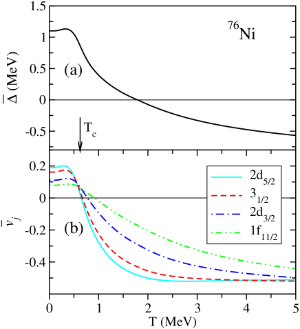
Figure 1: The MBCS pairing gap $\bar{\Delta}$ (upper part (a)) and $\bar{v}_{j}$ coefficients (lower part (b)) for particle levels near the Fermi surface in ⁷⁶Ni (neutrons). The conventional critical temperature $T_{c}$ is shown by the vertical arrow and the single particle spectrum used is from Ref. DA03a .

In calculations with a wider single-particle spectrum in Ni isotopes we have found that the gap starts to continuously increase above a certain temperature remaining always positive. The pairing strength has been renormalized to keep the $\bar{\Delta}(T=0)$ value.

An example of such behavior of the pairing gap is presented in Fig. 2(a) for ⁸⁴Ni. As can be seen, at $T\approx 3.3$ MeV some strange discontinuities are apparent, a phenomenon which may be defined as a “superfluid – super-superfluid” (S-SS) phase transition. At this temperature, the MBCS equations find a new energetically-preferable solution. A $T$-dependence of the total excitation energy given by

$${\rm E}^{*}={\cal E}(T)-{\cal E}(0),$$ (16)

where ${\cal E}(T)$ is calculated from Eq. (45) in Ref. DA03a , is shown in Fig. 2(c). The chemical potential jumps away from the $\lambda(T=0)$ value at $T\approx 3.3$ MeV (see Fig. 2(b)).

Figure 2: The MBCS pairing gap $\bar{\Delta}$ (upper part (a)), chemical potential $\bar{\lambda}$ (middle part (b)), and excitation energy ${\rm E}^{*}$ (lower part (c)) in ⁸⁴Ni (neutrons). Single particle spectrum from Ref. DA03a is extended by including levels from $N=0-28$ shells.

In short, while at the $\bar{\Delta}=0$ point the behavior of physical observables is smooth (see Fig. 1(b)), the discontinuities at the S-SS point in excitation energy, pairing gap and chemical potential take place. Thus, there is no phase transition from the superfluid to normal phase within the MBCS but instead a phase transition of a new type is predicted at finite temperatures.

The absence of the normal phase in all MBCS calculations has motivated us to apply this model to a magic-number system of nucleons in which the existence of this phase at $T=0$ is expected. The nucleus ¹²⁰Sn has been taken as an example. The MBCS neutron pairing gap (solid line in Fig. 3(a)) in this nucleus shows the same behavior as already discussed for ⁷⁶Ni even though a rather complete single particle basis has been employed in ¹²⁰Sn. The neutron pairing gap vanishes at $T\approx 5.5$ MeV and becomes negative at higher temperatures.

The proton gap in ¹²⁰Sn exhibits a rather strange behavior as a function of $T$. Starting from zero value at $T=0$ the gap smoothly develops to a value of $-0.73$ MeV at $T=5$ MeV (dashed line in Fig. 3(a)). A completely different result for the MBCS proton pairing gap in this nucleus has been reported in Ref. DA03b and it is shown as the dotted line $\bar{\Delta}_{\rm CS}$ in Fig. 3(a). To obtain it, it has been suggested that closed-shell systems should be treated differently from open-shell ones, namely, all summations in the MBCS equations (LABEL:MBCS2) should be carried over hole levels only.

Figure 3: The MBCS pairing gap $\bar{\Delta}$ (upper part (a)) and chemical potential $\bar{\lambda}$ (lower part (b)) for neutrons (solid lines) and protons (dashed lines) in ¹²⁰Sn. $\bar{\Delta}_{\rm CS}$ and $\bar{\lambda}_{\rm CS}$ (dotted lines) correspond to closed-shell calculations in Ref. DA03b . See text for details.

In our opinion, the last recipe contradicts the previous recipe of “entire spectrum” in the same publication. It is also evident that this artificial constraint cannot be justified for a heated system. Indeed, both subsystems, the former hole (fully occupied) and particle (empty) levels, become partially occupied due to the heating and there are no physical reasons to ignore the particle part of a single-particle spectrum. Moreover, to keep the number of nucleons $N$ constant under the above constraint, forces the MBCS equations to abnormally renormalize the corresponding chemical potential. In the above CS-calculations the $\bar{\lambda}$ quantity runs away from $\bar{\lambda}_{\pi,{\rm CS}}(T=0)=-10$ MeV to $\bar{\lambda}_{\pi,{\rm CS}}(T=5)=+175$ MeV (following the dotted line in Fig. 3(b)). In addition, the capacity of the system is zero in the CS-approximation, i.e. the system is artificially frozen.

The above MBCS results are natural consequences of Eqs. (LABEL:MBCS2). For example, these equations do not have the trivial solution $\{{\bar{u}}_{j},~{}{\bar{v}}_{j}\}=\{0(1),1(0)\}$. Indeed, from Eqs. (13) it would correspond to
         $u_{j}=\sqrt{1-n_{j}}$;      $v_{j}=\sqrt{\vphantom{1}n_{j}}$      – particles          $u_{j}=-\sqrt{\vphantom{1}n_{j}}$;      $v_{j}=\sqrt{1-n_{j}}$      – holes
and contradict the positive definition of $u_{j}$.

One may also notice from Eqs. (13) that ${\bar{v}_{j}}$ coefficients become negative for particle levels above a certain temperature, with $n_{j}$ increasing, since $v_{j}<<u_{j}$. In which case the MBCS pairing gap $\bar{\Delta}$ receives a positive contribution from hole levels and a negative contribution from particle levels. Thus, the contribution of single-particle and single-hole states to a pairing phenomenon appears to be essentially different.

Numeric calculations (see Fig. 1(b)) show that two terms in the second expression of Eqs. (LABEL:MBCS2) compensate each other around the critical temperature of the conventional BCS $T_{c}\approx 0.57\cdot\Delta_{T=0}$ for particle levels and ${\bar{v}_{j}}$ become negative at higher temperatures. The gap ${\bar{\Delta}}$ may vanish at some temperature but only when a negative contribution from particles and positive contribution from holes cancel each other (notice the difference with the conventional BCS $\Delta=0$). However if this happens, at higher $T$ the balance appears to be broken and ${\bar{\Delta}}$ becomes finite again. It also means that $\bar{\Delta}=0$ has nothing in common with the normal phase and that one cannot conclude from the absolute value of the pairing gap how strong the pairing is in the system.

The temperature behavior of the pairing gap depends on a delicate balance between particle- and hole-parts of the single-particle basis used which makes the MBCS predictions very doubtful.

IV MBCS and exact solutions of the pairing Hamiltonian

In this section we compare MBCS predictions with exact solutions of the pairing Hamiltonian employing the Picket Fence Model (PFM) PFM which is widely used as a test model for the pairing problem (see, e.g., Ref. sto ). For numeric calculations we have selected $N=10$ levels, each of two-fold degenerate (for spin up and spin down), with the energy difference of 1 MeV and 10 particles distributed over the levels. This configuration thus represents 5 levels for holes with energies $\varepsilon_{-i}=-0.5$ MeV, $-1.5$ MeV, etc and 5 levels for particles with energies $\varepsilon_{i}=+0.5$ MeV, $+1.5$ MeV, etc.

The MBCS predictions for the pairing gap, excitation energy, and specific heat given by

$$C_{\nu}=\frac{\partial{\cal E}}{\partial T}$$

are shown in Fig. 4 by the solid lines. Here, also shown are the FT-BCS results as dashed lines (explicit expressions for the quantity ${\cal E}$ in both approaches are given below). Both the MBCS and FT-BCS can be compared to the exact solutions of the pairing Hamiltonian (dotted lines). It should be noted that the MBCS-PFM pairing gap behavior is qualitatively very similar to the one in ⁸⁴Ni reported in Fig. 2(a) and that the “superfluid – super-superfluid” phase transition takes place at $T\approx 1.78$ MeV.

One concludes from Fig. 4 that the MBCS does not achieve its main goal of improving upon the description of heated nuclei in the conventional FT-BCS. Indeed, except for a narrow region around $T_{c}$, the deviation from the exact results is worse in the MBCS case compared to the conventional FT-BCS, which persists even at a very low temperature. It is also obvious that the “superfluid – super-superfluid” phase transition as well as the overall behavior at higher temperatures are artificial effects of the MBCS.

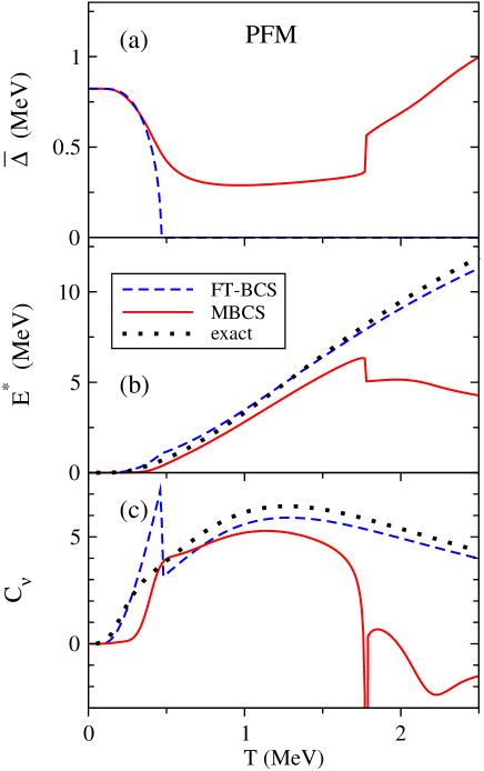
Figure 4: Pairing gap $\bar{\Delta}$ (upper part (a)), excitation energy ${\rm E}^{*}$ (middle part (b)), and specific heat (lower part (c)) $C_{\nu}$ as predicted by the MBCS (solid lines) and FT-BCS (dashed lines) for the PFM ($N=10$ and $G=0.4$ MeV). The exact results in (b) and (c) are plotted by dotted lines.

In addition, a more detailed analysis shows that the situation with the MBCS is much worse than the disagreement apparent in Fig. 4. We further present in Fig. 5 the spectroscopic factors for two particle and two hole levels closest to the Fermi surface, within the MBCS (solid lines) and FT-BCS (dashed lines) for a comparison with the exact results (dotted lines). It is important to keep in mind that the pairing Hamiltonian in the PFM possesses particle-hole symmetry. For this reason, dotted curves in Fig. 5 for hole $-i$ and particle $i$ levels are ideally symmetric about the $y=1$ line. The same is true for the FT-BCS results. Nothing of this symmetry remains after the secondary Bogoliubov transformation of Eq. (9) is applied in the MBCS (see solid lines in the same figure). In addition, the description of this physical observable in the MBCS is very poor compared to the FT-BCS results.

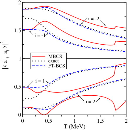
Figure 5: Spectroscopic factors of two lowest particle and hole levels in the PFM ($N=10$ and $G=0.4$ MeV) calculated within the MBCS (solid lines) and FT-BCS (dashed lines). Dotted lines represent the exact results.

Breaking of the particle-hole symmetry in the MBCS calculations is even more clearly seen from an analysis of the MBCS quasiparticle spectrum presented in Fig. 6(b). In the PFM it should be two-fold degenerate (i.e. $\bar{E_{i}}\equiv\bar{E}_{-i}$) as, e.g., in the FT-BCS calculation in Fig. 6(a) because of this symmetry. The chemical potential $\bar{\lambda}$ in the MBCS calculations does not stay at zero energy (as it should be) but runs away to positive values as temperature increases. This explains why the level $i=2$ appears at a lower energy than the $i=1$ level above $T\approx 1.6$ MeV. It is also the origin of the $E_{i}/E_{-i}$ splitting in these calculations.

We have repeated the MBCS-PFM calculations with different values of the pairing strength $G>G_{\rm cr}$. As $G$ increases, the MBCS “superfluid – super-superfluid” phase transition takes place at a lower temperature and the splitting of $i$ and $-i$ levels becomes stronger.

Another consequence of the particle-hole symmetry is that under any conditions it should be true that $u_{i}\equiv v_{-i}$ and $v_{i}\equiv u_{-i}$ or alternatively

$$u_{i}^{2}+u_{-i}^{2}\equiv u_{i}^{2}+v_{i}^{2}=1\ .$$ (17)

In Fig. 7 we demonstrate what happens to this analytical identity in the MBCS. The calculations have been performed for a different number of levels $N$ of the PFM and the strength parameter G has been adjusted to keep $T_{c}=0.5$ MeV in each calculation. The convergence of the results in this $T$-range (also for $\bar{\Delta}$, $\bar{\lambda}$, and $E^{*}$) is reached at $N\approx 10$. The conclusion from Fig. 7 is that the analytical identity of Eq. (17) is completely broken in MBCS calculations even from very low temperatures.

Figure 6: Quasiparticle spectrum in the PFM ($N=10$ and $G=0.4$ MeV) within the FT-BCS (upper part (a)) and the MBCS (lower part (b)). Particle (hole) levels are plotted by thick (thin) lines.

Figure 7: The $(u_{1}^{2}+u_{-1}^{2})$ quantity in the MBCS-PFM calculations with different $N$. $T_{c}=0.5$ MeV is the same in all calculations. Analytical identity (y=1) is plotted as a dotted line.

Thus, one can see that the MBCS severely violates the symmetry between particles and holes which is an essential feature of the pairing problem solved for the PFM. Accordingly, the MBCS can be applied to this problem only at temperatures much lower than $T_{c}$.

V Inconsistencies of MBCS and MHFB approaches

In this section the evaluation of the MBCS equations is analyzed to verify consistency. To start with we agree that the pairing Hamiltonian $\bar{H^{\prime}}$ expressed via the MBCS variables $\bar{u}_{j}$ and $\bar{v}_{j}$ has the same form as the BCS Hamiltonian $H^{\prime}$ of Eq. (5) at $T=0$. It is also true that the expectation value of the pairing Hamiltonian $\langle\bar{0}|H_{\rm pair}|\bar{0}\rangle$ at $T\neq 0$ looks similar to $\langle 0|H_{\rm pair}|0\rangle$ in the case of the BCS at $T=0$. But then the formal similarity is broken and the corresponding energies $\bar{E}_{j}$ are attributed to the conventional Bogoliubov quasiparticles and not to the “bar”-quasiparticles. These energies $\bar{E}_{j}=\sqrt{(\varepsilon_{j}-\bar{\lambda})^{2}+\bar{\Delta}^{2}}$ enter through new thermal occupation numbers $n_{j}$ and new $u,v$-coefficients

$$u_{j}=\sqrt{\frac{1}{2}\left(1+\frac{\varepsilon_{j}-\bar{\lambda}}{\bar{E}_{j}}\right)},~{}~{}~{}v_{j}=\sqrt{\frac{1}{2}\left(1-\frac{\varepsilon_{j}-\bar{\lambda}}{\bar{E}_{j}}\right)}$$ (18)

(see remarks on page 8 in Ref. DA03b just after Eq. (86)).

In another words, the MBCS procedure yields new eigen energies of Bogoliubov quasiparticles while new eigen states are now modified quasiparticles. The point here is that if one would take the mean of the modified quasiparticle energies under $\bar{E}_{j}$, they should coincide with the BCS $E_{j}$ at $T=0$. Indeed, the secondary Bogoliubov transformation of Eq. (9) is a unitary one and as such, cannot change the eigenvalues of the Hamiltonian.

There are several possibilities to derive analytically the BCS equations from the expectation value $\langle 0|H_{\rm pair}|0\rangle$ at $T=0$. One of them is presented, e.g., in Ref. ho . The BCS equations are obtained by demanding that

$$b_{j}\equiv E_{j}~{}~{}~{}{\rm and}~{}~{}~{}c_{j}\equiv 0,$$ (19)

where $b_{j}$ and $c_{j}$ are defined in Eqs. (II). The first expression in Eqs. (19) means that the pairing Hamiltonian is diagonalized in the quasiparticles space, the second one indicates that the so-called “dangerous diagrams” are excluded from the theory. The solution of the BCS equations is unique. In another words, it is absolutely necessary that Eqs. (19) are fulfilled exactly to have the BCS equations in the form given in Eq. (3). Let us verify this for the MBCS.

We introduce ${\bar{b}_{j}}$ and ${\bar{c}_{j}}$ quantities to replace the $\{u_{j},v_{j}\}$ coefficients in Eqs. (II) by $\{\bar{u}_{j},\bar{v}_{j}\}$ coefficients and calculate the later from the MBCS equations. The differences $|\bar{b}_{j}-\bar{E}_{j}|$ and ${\bar{c}_{j}}$ quantities for several neutron sub-shells in ¹²⁰Sn are presented in Fig. 8(a) and Fig. 8(b), respectively, showing that

$$\bar{b}_{j}\neq\bar{E}_{j}~{}~{}~{}{\rm and}~{}~{}~{}\bar{c}_{j}\neq 0~{}.$$ (20)

In addition, Eqs. (19) are also not fulfilled within the MBCS.

We remind a reader that the MBCS equations were not obtained analytically but were written down in analogy with the $T=0$ BCS equations and, as far as the MBCS founders had noticed, using a formal similarity in some BCS and MBCS expressions. But, as a matter of fact, the basic MBCS equations contained in Eqs. (14) or Eqs. (LABEL:MBCS2) cannot be reached from the expectation value $\langle\bar{0}|H_{\rm pair}|\bar{0}\rangle$ at finite $T$ because Eqs. (20).

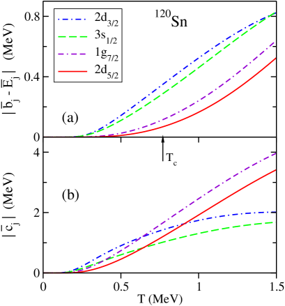
Figure 8: The MBCS $\bar{b}_{j}$ and $\bar{c}_{j}$ quantities as functions of temperature for some neutron levels in ¹²⁰Sn. See text for details.

One finds in the literature DA03b that the MBCS equations may be obtained from a modified HFB model called the MHFB. Here, it was noticed that after application of the secondary Bogoliubov transformation of Eq. (9), a generalized particle-density matrix at finite temperature “formally looks the same as the usual HFB approximation at $T=0$” DA03b . Then, “following the rest of the derivation as for the zero-temperature case” DA03b , the MHFB equations were written down. Below we verify thermodynamical consistency of the MHFB (MBCS) since Ref. DA03b lacks such an analysis.

The total energy of the system in the statistical approach has the form

$$<{\rm H}>={\rm Tr}(HD),$$ (21)

where $D$ is a density operator and $<\ldots>$ means averaging over the grand canonical ensemble. After grand potential minimization, one obtains an expression for the system energy as

$${\cal E_{\rm BCS}}=2\sum_{j}\Omega_{j}\varepsilon_{j}\left[(1-2n_{j})v^{2}_{j}+n_{j}\right]-\Delta^{2}/G$$ (22)

in the FT-HFB (or FT-BCS). In the MHFB (or MBCS) it has the form

$${\cal E_{\rm MBCS}} = 2\sum_{j}\Omega_{j}\varepsilon_{j}\left[(1-2n_{j})v^{2}_{j}+n_{j}\right.$$ (23)

$$- \left.2\sqrt{n_{j}(1-n_{j})}~{}u_{j}v_{j}\right]-\bar{\Delta}^{2}/G~{}.$$

Equation (23) appears as Eq. (83) in Ref. DA03b or as Eq. (45) in Ref. DA03a .

In Fig. 9(a) we present the low-$T$ part of Fig. 4(b) (up to $T_{c}$) with predictions of the MBCS (solid lines) and FT-BCS (dashed lines) for the system excitation energy. It should be reminded that the results in Fig. 4(b) were obtained for the ${\rm E}^{*}$ quantity (see Eq. (16)) with ${\cal E}$ calculated in the MBCS and FT-BCS from Eq. (23) and Eq. (22), respectively. These results are plotted by thick lines in Fig. 9(a). The excitation energy calculated in the MHFB and FT-HFB as

$$<{\rm H}>^{*}=<{\rm H}>(T)-<{\rm H}>(0)$$

(in the $G_{jj^{\prime}}=G$ limit for exact comparison with the MBCS and FT-BCS results) is shown by thin lines in the same figure. Since $D_{\rm MHFB}$ (Eq. (66) in Ref. DA03b ) does not equal $D_{\rm HFB}$ (Eq. (12) in Ref. DA03b ), the $<{\rm H}>_{\rm MHFB}^{*}$ and $<{\rm H}>_{\rm HFB}^{*}$ quantities are slightly different in Fig. 9.

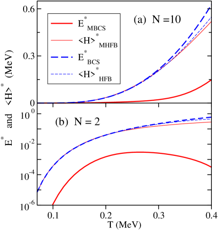
Figure 9: Excitation energy of the PFM calculated as ${\rm E}^{*}$ (thick lines) and $<{\rm H}>^{*}$ (thin lines) in the MHFB (solid lines) and the FT-HFB (dashed lines) with $T_{c}=0.42$ MeV for $N=10$ (upper part (a)) and $N=2$ (lower part (b)).

In any consistent model the values $<{\rm H}>^{*}$ and ${\rm E}^{*}$ should not differ significantly since they represent the same physical observable. One notices that the accuracy of the FT-BCS becomes worse on approaching $T_{c}$ as is well known, and disagreement reaches a few percent. The picture within the MHFB (MBCS) is completely different: the ${\rm E}^{*}_{\rm MBCS}$ quantity is several times smaller than the $<{\rm H}>^{*}_{\rm MHFB}$ quantity almost at any $T$ in this example footnote . We have repeated the calculations in Fig. 9(a) also for $N=8$ and 12 keeping $T_{c}$ fixed. The differences between the $N=8,$ 10, and 12 results are hardly noticed by eye for each line in Fig. 9(a), i.e. convergence of the results in this example is reached with $N=8-10$. The correspondence between $<{\rm H}>^{*}$ and ${\rm E}^{*}$ remains still acceptable for the FT-HFB (FT-BCS) even for $N=2$ (see Fig. 9(b)). On the other hand, disagreement in the MHFB (MBCS) results reaches several orders of magnitude in the $N=2$ case (notice logarithmic y-scale in Fig. 9(b)).

To conclude, thermodynamical inconsistency of the MHFB (MBCS) is obvious from this example. This inconsistency is detected from $T<<T_{c}$.

The last result clearly demonstrates that the MBCS approach is not justified in the framework of the usual statistical approach. This conclusion can be reached by other reasoning as well. The point is that the basic MBCS equations given by Eqs. (LABEL:MBCS2) obtained via the secondary Bogoliubov transformation cannot be considered as a result of the thermal averaging over the grand canonical ensemble. Indeed, the bar-quasiparticles in Eq. (9) and the new correlated ground state

$$|\bar{0}\rangle=\prod_{jm}\left(\sqrt{1-n_{j}}+\sqrt{n_{j}}\alpha^{+}_{jm}\alpha^{+}_{j\tilde{m}}\right)|0\rangle$$

are temperature dependent although the MBCS founders do not use this terminology. A possibility to deduce the basic MBCS equations via a variational procedure in application to the average value $\langle\bar{0}|H|\bar{0}\rangle$ contradicts what was proven long ago tak : a ground state with such a property cannot be constructed in principle in the space spanned by eigenvectors of a quantum Hamiltonian (see also footnote on page 3 in Ref. DA03a ).

VI Conclusions

In this article we have studied the modified BCS model suggested and explored in a series of papers DZ01 ; DA03a ; DA03b ; DA03c ; DA03d . We have shown that this model yields many unphysical predictions: a negative value for the pairing gap, the pairing correlations induced by heating in the closed-shell systems, the “superfluid – super-superfluid” phase transition. It also predicts that the normal phase does not exist at any finite temperature. The MBCS has been tested on the picket fence model for which an exact solution of the pairing problem is available. In addition to rather poor description of the exact solutions, it has been found that the model severely violates the internal particle-hole symmetry of the problem.

Analysis of the MBCS equations, their derivation, and description of different physical observables by this model have led us to the following general conclusion: The $T$-range of the MBCS applicability has been determined to be far below the conventional critical temperature $T_{c}$. Within this narrow temperature interval the MBCS performance is worse in comparison with that of the conventional FT-BCS. Moreover, the MBCS is found to be thermodynamically inconsistent.

References

- (1) D.J. Dean and M. Hjorth-Jensen, Rev. Mod. Phys. 75, 607 (2003).
- (2) V. Zelevinsky and A. Volya, arXiv: nucl-th/0303010, 2003.
- (3) N. Dinh Dang and V. Zelevinsky, Phys. Rev. C 64, 064319 (2001).
- (4) N. Dinh Dang and A. Arima, Phys. Rev. C 67, 014304 (2003).
- (5) N. Dinh Dang and A. Arima, Phys. Rev. C 68, 014318 (2003).
- (6) N. Dinh Dang and A. Arima, Phys. Rev. C 68, 044303 (2003).
- (7) N. Dinh Dang and A. Arima, Nucl. Phys. A722, 383c (2003).
- (8) J. Högaasen-Feldman, Nucl. Phys. 28, 258 (1961).
- (9) R.W. Richardson and N. Sherman, Nucl. Phys. A52, 221 (1964).
- (10) A. Storozhenko, P. Schuck, J. Dukelsky, G. Röpke, and A. Vdovin, Ann. Phys. 307, 308 (2003).
- (11) Very small, almost zero, and values for is a distinctive feature of other MBCS predictions as well (see Fig. 2 above and Fig. 4 in Ref. DA03a ). Rather different behavior of the value at low in the MBCS is reported in Fig. 8a of Ref. DA03b for 120Sn. How it has been obtained and why it is so different from similar calculations in Ni isotopes in Ref. DA03a by the same authors, remains unclear to us. Among what we have checked, this is the only result from all previously published MBCS predictions which we did not manage to reproduce.
- (12) Y. Takahashi and H. Umezawa, Collect. Phenom. 2, 55 (1975).