Pairing properties of nucleonic matter employing dressed nucleons

Abstract

A survey of pairing properties of nucleonic matter is presented that includes the off-shell propagation associated with short-range and tensor correlations. For this purpose, the gap equation has been solved in its most general form employing the complete energy and momentum dependence of the normal self-energy contributions. The latter correlations include the self-consistent calculation of the nucleon self-energy that is generated by the summation of ladder diagrams. This treatment preserves the conservation of particle number unlike approaches in which the self-energy is based on the Brueckner-Hartree-Fock approximation. A huge reduction in the strength as well as temperature and density range of ${}^{3}S_{1}$-${}^{3}D_{1}$ pairing is obtained for nuclear matter as compared to the standard BCS treatment. Similar dramatic results pertain to ${}^{1}S_{0}$ pairing of neutrons in neutron matter.

I INTRODUCTION

Advances in the understanding of the single-particle (sp) properties of nucleons in nuclei and nuclear matter diba04 demonstrate the dominant influence of short-range and tensor correlations in generating the distribution of the spectral strength. One aspect of this influence is expressed in the global depletion of Fermi sea due to these correlations. A recent experiment from NIKHEF puts this depletion of the proton Fermi sea in ²⁰⁸Pb at a little less than 20% bat01 in accordance with earlier nuclear matter calculations vond1 . Another consequence of the presence of short-range and tensor correlations is the appearance of high-momentum components in the ground state to compensate for the depleted strength of the mean field. Recent JLab experiments rohe:04 indicate that the amount and location of this strength is consistent with earlier predictions for finite nuclei mudi:94 and calculations for infinite matter frmu:03 ; thesfr . Of particular relevance is the observed energy distribution of the sp strength of the high-momentum nucleons that is located at energies far removed from the Fermi energy. This situation is similar to the case of nuclear matter vond2 and also holds above the Fermi energy. Such sp strength distributions lead to substantial modifications of the calculated properties of low-energy phenomena, like pairing, as compared to those generated by a traditional mean-field treatment.

Pairing properties of nuclear and neutron matter have been studied for quite some time. A recent review can be found in Ref. dehj:03 . The study of pairing correlations in infinite quantum systems is an interesting question in general relating nuclear and neutron matter to the classical systems studied in condensed matter physics as well as to the studies of pairing correlations in fermionic atomic gases qijn:05 . The study of pairing correlations in nuclear and neutron matter is of particular interest for the understanding of properties of neutron stars. The formation of a BCS gap has a significant effect on the neutrino emissivity, which is crucial for the cooling of neutron stars bla:05 . The existence of superfluid layers will affect the rotation of neutron stars.

Of particular interest is the observation that several calculations for the bare nucleon-nucleon (NN) interaction in the ${}^{3}S_{1}$-${}^{3}D_{1}$ coupled channel lead to a sizable gap of around 10 MeV at normal nuclear matter density ars:90 ; vgdpr:91 ; bbl:92 ; tt:93 ; bls:95 . Those calculations typically solve the BCS gap equation using a mean-field sp propagator with sp energies as determined e.g. in a Brueckner-Hartree-Fock (BHF) calculation.

The empirical data of finite nuclei do not exhibit any indications for such strong proton-neutron pairing correlations, which would correspond to a gap as large as 10 MeV. Therefore one may conclude that such evaluations of a pairing gap in infinite matter yield quite different results from those observed for finite nuclei. This appears plausible since pairing effects are very sensitive to the sp spectrum close to the Fermi energy, which is continuous in infinite matter while it is discrete in finite nuclei.

This observation may also cast some doubt on the reliability of the approach to determine the pairing gap for infinite matter as outlined above. Therefore attempts have been made to go beyond this mean-field approach. One issue discussed in the literature has been the role of vertex corrections, i.e. the medium dependence of the NN interaction to be used in solving the gap equation ZLS:02 ; sedr:03 ; sls:03 ; sls:05 . Using effective interactions like the Gogny force gogny Shen et al. sls:03 ; sls:05 observe indeed a significant effect, which is larger for nuclear matter than for neutron matter. The effects of the so-called induced interaction could indeed affect the low-energy spectroscopy of nuclear matter in a significant way. Before conclusions can be drawn, calculations employing realistic interactions should be performed, which, unfortunately, are very difficult induced . In addition, it is possible that polarization effects are different in nuclear matter and finite nuclei on account of the difference of the sp spectra discussed above.

In the present work we would like to focus the attention to the study of pairing correlations with a proper treatment of the nucleon propagator that accounts for the effects of short-range and tensor correlations. The crucial effects of short-range and tensor correlations on the distribution of the sp strength have recently been treated at a very sophisticated level. Various groups have developed techniques to evaluate the sp strength from realistic NN interactions, like the Argonne V18 arv18 or the CDBonn cdbonn interaction, within the self-consistent Green’s function (SCGF) approach rd ; dwvnw ; bozek0 ; bozek1 ; bozek2 ; dewulf:03 ; frmu:03 ; diep:03 ; frmu:05 . Such calculations reproduce the energy- and momentum-distribution of the sp strength corresponding to high-momentum nucleons as observed in experiments rohe:04 and account for the depletion of the mean-field strength obtained in bat01 .

In these calculations the scattering equations for two nucleons in the medium are solved employing dressed sp propagators that contain the complete information about the energy- and momentum-distribution of the sp strength. The resulting scattering matrix $T$ is then used to calculate the nucleon self-energy. The solution of the Dyson equation, employing this complex and energy dependent self-energy, yields the sp propagator that enters the $T$ matrix equation to close the self-consistency cycle. In determining the two-nucleon Green’s function or the corresponding scattering matrix $T$, one has to face the problem of the so-called pairing instabilities that reflect the existence of NN bound state solutions in the scattering equation. The presence of such solutions provides a major numerical obstacle for a self-consistent evaluation of one- and two-body propagator within the normal Green’s function approach at densities where such instabilities can occur. For this reason, recent SCGF calculations have been performed for temperatures above the critical temperature for a possible phase transition to pairing condensation rd ; frmu:03 .

In Sec. II of this work we will review some basic features of the SCGF method for the normal Green’s function at temperatures above the critical one for the pairing instability. The effects of the anomalous Green’s functions will be considered in Sec¿ III. This leads to the generalized gap equation that corresponds to the homogeneous scattering equation for dressed nucleons. The analogous problem occurs for two nucleons in the vacuum, where the solution of the homogeneous scattering equation yields the description of the bound two-nucleon state, the deuteron. In the nuclear medium, however, one has to consider a scattering equation with dressed sp propagators. If one considers the HF or BHF approximation for the normal sp propagator, in which the spectral function is replaced by a $\delta$-function, this gap equation reduces to the usual BCS approximation.

Results of SCGF calculations above the critical temperature will be discussed in Sec. IV. We will pay special attention to the spectral functions associated with sp strength around the Fermi energy and discuss, to which extend these exhibit typical precursor phenomena for a phase transition to a pairing condensate schnell:99 . In Sect. IV we will also investigate how the distribution of the sp strength modifies the solution of the gap equation and the subsequent predictions for a phase transition to a superfluid state of nuclear matter. Such investigations have been performed before by Bozek boz:99 ; boz:03 using simplified models for the NN interaction. These studies suggest an important sensitivity to these correlations, accompanied by a substantial suppression of the strength of pairing. A similar conclusion was reached for a realistic interaction in Ref. dick:99 by studying the phase shifts of dressed nucleons in the medium that signal the presence of bound pair states as in the case of two free particles. The inclusion of dressing effects in the study of pairing has also been studied in Refs. bagr:00 ; lsz:01 ; blsz:02 based on the hole-line expansion of the nucleon self-energy. While also in this work a substantial reduction of the strength of pairing is observed, the implementation of the scheme to solve the gap equation relies on approximations that do not conserve particle number, since they involve the introduction of quasiparticle strength factors to represent the effect of dressing. Final conclusions are drawn in Sec. V.

II GREEN’S FUNCTIONS AND T-MATRIX APPROXIMATION

One of the key quantities within the SCGF approach is the sp Green’s function, which can be defined in a grand-canonical formulation for both real and imaginary times $t$, $t^{\prime}$ kadanoff :

$${\mathrm{i}}G({\mathbf{x}},t;{\mathbf{x}}^{\prime},t^{\prime})=\frac{{\mathrm{tr}}\{\exp[-\beta(H-\mu N)]{\cal{T}}[\psi({\mathbf{x}}t)\psi^{\dagger}({\mathbf{x}}^{\prime}t^{\prime})]\}}{{\mathrm{tr}}\{\exp[-\beta(H-\mu N)]\}}\,,$$ (1)

where $\cal{T}$ is the time ordering operator, $\beta$ the inverse temperature, and $\mu$ the chemical potential of the system. Due to the invariance of the trace under cyclic permutations the one-particle Green’s function obeys the following quasi-periodicity condition

$$G({\mathbf{x}},t=0;{\mathbf{x}}^{\prime},t^{\prime})=-e^{\beta\mu}G({\mathbf{x}},t=-{\mathrm{i}}\beta;{\mathbf{x}}^{\prime},t^{\prime}).$$ (2)

For a system invariant under translation in space and time, the propagator depends only on the differences $|{{\mathbf{x}}-{\mathbf{x}}^{\prime}}|$ and $t-t^{\prime}$, allowing a Fourier transformation into momentum and energy variables $k$ and $\omega$. Due to the quasi-periodicity in Eq. (2), the Green’s function can be expressed in terms of the Fourier coefficients $G(k,z_{\nu})$, where $z_{\nu}=\frac{\pi\nu}{-{\mathrm{i}}\beta}$ are the (fermion) Matsubara frequencies with odd integers $\nu$. Since these are related to the spectral function $A(k,\omega)$ by

$$G(k,z_{\nu})=\int_{-\infty}^{+\infty}\frac{{\mathrm{d}}\omega}{2\pi}\,\frac{A(k,\omega)}{z_{\nu}-\omega}\,,$$ (3)

$G(k,z_{\nu})$ can be continued analytically to all non-real $z$. On the other hand, the spectral function is related to the imaginary part of the retarded propagator $G(k,\omega+{\mathrm{i}}\eta)$ by

$$A(k,\omega)=-2\,{\mathrm{Im}}\,G(k,\omega+{\mathrm{i}}\eta)\,.$$ (4)

In the limit of the mean-field or quasi-particle approximation the spectral function is represented by a $\delta$-function and takes the simple form

$$A(k,\omega)=2\pi\delta(\omega+\mu-\varepsilon_{k})=2\pi\delta(\omega-\chi_{k})\,,$$ (5)

with the quasi-particle energy $\varepsilon_{k}$ for a particle with momentum $k$ and $\chi_{k}=\varepsilon_{k}-\mu$. Note, that for convenience we define the energy variable relative to the chemical potential $\mu$.

The sp Green’s function is obtained as a solution of the Dyson equation, which, for a translationally invariant system, is a simple algebraic equation

$$\left[\omega+\mu-\frac{k^{2}}{2m}-\Sigma(k,\omega)\right]G(k,\omega)=1\,,$$ (6)

where $\Sigma(k,\omega)$ denotes the complex self-energy. By expanding the self-energy in terms of one-particle Green’s functions it can be demonstrated that it inherits all analytic properties of $G$. It it thus possible to write

$$\Sigma(k,\omega)=\Sigma^{HF}(k)-\frac{1}{\pi}\int_{-\infty}^{+\infty}{\mathrm{d}}\omega^{\prime}\,\frac{{\mathrm{Im}}\Sigma(k,\omega^{\prime}+{\mathrm{i}}\eta)}{\omega-\omega^{\prime}}.$$ (7)

The next step is to obtain the self energy in terms of the in-medium two-body scattering $T$ matrix. It is possible to express ${\mathrm{Im}}\Sigma(k,\omega+{\mathrm{i}}\eta)$ in terms of the retarded $T$ matrix kadanoff ; frmu:03

$${\mathrm{Im}}\Sigma(k,\omega+{\mathrm{i}}\eta) = \frac{1}{2}\int\frac{{\mathrm{d}}^{3}k^{\prime}}{(2\pi)^{3}}\int_{-\infty}^{+\infty}\frac{{\mathrm{d}}\omega^{\prime}}{2\pi}\left<{\mathbf{kk}}^{\prime}|{\mathrm{Im}}T(\omega+\omega^{\prime}+{\mathrm{i}}\eta)|{\mathbf{kk}}^{\prime}\right>$$ (8)

$$\qquad\times[f(\omega^{\prime})+b(\omega+\omega^{\prime})]A(k^{\prime},\omega^{\prime}).$$

Here and in the following

$$f(\omega) = \frac{1}{e^{\beta\omega}+1}\,,$$

$$b(\Omega) = \frac{1}{e^{\beta\Omega}-1}\,,$$ (9)

denote the Fermi and Bose distribution functions, respectively. The pole in the Bose function $b(\Omega)$ at $\Omega=0$ is compensated by a corresponding zero in the $T$ matrix alm1 ; alm95 such that the integrand remains finite as long as the $T$ matrix does not acquire a pole at this energy. Such a pole may occur below a critical temperature $T_{C}$, a phenomenon that is often referred to as a pairing instability. We will come back to this problem below.

The scattering matrix $T$ is to be determined as a solution of the integral equation

$$\left<{\mathbf{kk}}^{\prime}|T(\Omega+{\mathrm{i}}\eta)|{\mathbf{pp}}^{\prime}\right> = \left<{\mathbf{kk}}^{\prime}|V|{\mathbf{pp}}^{\prime}\right>+\int\frac{d^{3}q\,d^{3}q^{\prime}}{\left(2\pi\right)^{6}}\left<{\mathbf{kk}}^{\prime}|V|{\mathbf{qq}}^{\prime}\right>G^{0}_{\mathrm{II}}(\mathbf{qq}^{\prime},\Omega+i\eta)$$ (10)

$$\quad\quad\times\left<{\mathbf{qq}}^{\prime}|T(\Omega+{\mathrm{i}}\eta)|{\mathbf{pp}}^{\prime}\right>\,,$$

where

$$G^{0}_{\mathrm{II}}(k_{1},k_{2},\Omega+i\eta)=\int_{-\infty}^{+\infty}\frac{{\mathrm{d}}\omega}{2\pi}\int_{-\infty}^{+\infty}\frac{{\mathrm{d}}\omega^{\prime}}{2\pi}A(k_{1},\omega)A(k_{2},\omega^{\prime})\frac{1-f(\omega)-f(\omega^{\prime})}{\Omega-\omega-\omega^{\prime}+i\eta}\,.$$ (11)

stands for the two-particle Green’s function of two non-interacting but dressed nucleons.

The Green’s function method yields a hierarchy of relations for the $N$-particle Green’s functions. The Dyson equation for the one-particle Green’s function involves the two-body potential as well as the two-particle Green’s function $G_{\mathrm{II}}({\mathbf{x}},t;\cdots;{\mathbf{x}}^{\prime\prime\prime},t^{\prime\prime\prime})$. In general, the equation of motion for the $N$-particle propagator will be coupled to the $(N+1)$-particle propagator, if the Hamiltonian contains a two-body interaction. In the self-consistent $T$-matrix approach, as outlined above, one ignores the effects of $N$-particle Green’s functions with $N$ larger equal to three, but solves the coupled equations for the one- and two-body Green’s functions in a self-consistent way.

In order to allow for an efficient solution of the two-body scattering equation, one expresses the two-particle Green’s function in (11) as a function of the total momentum ${\mathbf{P}}=\frac{1}{2}({\mathbf{k_{1}}}+{\mathbf{k_{2}}})$ and the relative momentum ${\mathbf{q}}=\frac{1}{2}({\mathbf{k_{1}}}-{\mathbf{k_{2}}})$. Using the usual angle-average approximation for the angle between ${\mathbf{P}}$ and ${\mathbf{q}}$ (see e.g. angleav for the accuracy of this approximation), the two-particle Green’s function can be written as a function of the length of these two-vectors, $P$ and $q$, only. This approximation leads to a decoupling of partial waves with different total angular momentum $J$. Therefore the integral equation (10) reduces to an integral equation in only one dimension of the form

$$\left<q|T^{JST}_{ll^{\prime}}(P,\Omega+{\mathrm{i}}\eta)|q^{\prime}\right> = \left<q|V^{JST}_{ll^{\prime}}|q^{\prime}\right>+\sum_{l^{\prime\prime}}\frac{2}{\pi}\int_{0}^{\infty}{\mathrm{d}}k^{\prime}\,k^{\prime 2}\left<q|V^{JST}_{ll^{\prime\prime}}|k^{\prime}\right>G^{0}_{\mathrm{II}}(P,\Omega+{\mathrm{i}}\eta,k^{\prime})$$ (12)

$$\quad\quad\times\left<k^{\prime}|T^{JST}_{l^{\prime\prime}l^{\prime}}(P,\Omega+{\mathrm{i}}\eta)|q^{\prime}\right>.$$

The summation of the partial waves,

$$\left<{\mathbf{kk}}^{\prime}\right|{\mathrm{Im}}\,T(\Omega+{\mathrm{i}}\eta)\left|{\mathbf{kk}}^{\prime}\right>=\frac{1}{4\pi}\sum_{(JST)l}(2J+1)(2T+1)\left<q({\mathbf{k}},{\mathbf{k}}^{\prime})\right|{\mathrm{Im}}\,T^{JST}_{ll}(P({\mathbf{k}},{\mathbf{k}}^{\prime}),\Omega+{\mathrm{i}}\eta)\left|q({\mathbf{k}},{\mathbf{k}}^{\prime})\right>,$$ (13)

yields the $T$ matrix in the form that is needed in Eq. (8). Finally, the Hartree-Fock contribution has to be added to the real part of $\Sigma$

$$\Sigma^{HF}(k)=\frac{1}{8\pi}\sum_{(JST)l}(2J+1)(2T+1)\int\frac{{\mathrm{d}}^{3}k^{\prime}}{(2\pi)^{3}}\left<q({\mathbf{k}},{\mathbf{k}}^{\prime})\right|V^{JST}_{ll}\left|q({\mathbf{k}},{\mathbf{k}}^{\prime})\right>n(k^{\prime}),$$ (14)

where $n(k)$ is the correlated momentum distribution

$$n(k)=\int_{-\infty}^{+\infty}\frac{{\mathrm{d}}\omega}{2\pi}f(\omega)A(k,\omega).$$ (15)

Note, that Eq. (14) corresponds to a generalized Hartree-Fock contribution, since the full one-particle spectral function is employed.

III PAIRING IN THE T-MATRIX APPROXIMATION

For temperatures below the critical temperature for a transition to a superfluid one has to supplement the evaluation of the normal Green’s function $G(k,\omega)$ with the anomalous Green’s function $F(k,\omega)$. While the self-consistent inclusion of ladder diagrams has reached quite a sophistication, it remains to fully account for the possibility of a pairing solution in such calculations for realistic NN interactions. In this paper we present a first step towards such a complete scheme by including the full self-consistent dressing due to normal self-energy terms generated by ladder diagrams, in the calculation of the anomalous self-energy and the solution of the corresponding generalized gap equation.

The inclusion of the anomalous Green’s function $F(k,\omega)$ yields a modification of the normal Green’s function in the superfluid phase that can be written as migdal ; schrieffer ; mahan ; diva:05

$$G_{s}(\mathbf{k},\omega+i\eta) = G(\mathbf{k},\omega+i\eta)-G(\mathbf{k},\omega+i\eta)\Delta(\mathbf{k})F(\mathbf{k},\omega+i\eta)$$

$$F(\mathbf{k},\omega+i\eta) = G(-\mathbf{k},-\omega-i\eta)G_{s}(\mathbf{k},\omega+i\eta)\Delta(\mathbf{k})\,.$$ (16)

under the assumption that the anomalous part of self-energy $\Delta$ does not depend on the energy. Therefore the full Green’s function can be obtained as

$$G_{s}(\mathbf{k},\omega+i\eta)=\frac{1}{G(\mathbf{k},\omega+i\eta)^{-1}+\Delta^{2}(\mathbf{k})G(-\mathbf{k},-\omega-i\eta)}\,.$$ (17)

These equations must be supplemented with the definition of the anomalous self-energy

$$\Delta(\mathbf{p})=\int\frac{d\omega}{2\pi}\int\frac{d^{3}k}{\left(2\pi\right)^{3}}\left<\mathbf{p}|V|\mathbf{k}\right>2{\mathrm{Im}}F(\mathbf{k},\omega+i\eta)f(\omega)\,.$$ (18)

If one employs Eq. (16) and uses the representation of the Green’s function $G$ in terms of the spectral function in Eqs. (3) and (4), supplemented by a corresponding definition of a spectral function for the total Green’s function

$$A_{s}(k,\omega)=-2\,{\mathrm{Im}}\,G_{s}(k,\omega+{\mathrm{i}}\eta)\,,$$ (19)

the expression for the self-energy $\Delta$ can be rewritten boz:99 in a partial wave expansion

$$\Delta^{JST}_{l}(p)=\sum_{l^{\prime}}\frac{2}{\pi}\int_{0}^{\infty}{\mathrm{d}}k\,k^{2}\int_{-\infty}^{+\infty}\frac{{\mathrm{d}}\omega}{2\pi}\int_{-\infty}^{+\infty}\frac{{\mathrm{d}}\omega^{\prime}}{2\pi}\left<p|V^{JST}_{ll^{\prime}}|k\right>A(k,\omega)A_{s}(k,\omega^{\prime})\frac{1-f(\omega)-f(\omega^{\prime})}{-\omega-\omega^{\prime}}\Delta^{JST}_{l^{\prime}}(k)\,.$$ (20)

If we ignore for a moment the difference between the spectral functions $A$ and $A_{s}$, we see that this equation for the self-energy $\Delta$ corresponds to the homogeneous scattering equation for the $T$-matrix in (10) at energy $\Omega=0$ and center-of-mass momentum $P=0$. This means that a non-trivial solution of Eq. (20) is obtained if and only if the scattering matrix $T$ generates a pole at energy $\Omega=0$, which reflects a bound two-particle state. This is precisely the condition for the pairing instability discussed above, demonstrating that this treatment of pairing correlations is compatible with the $T$-matrix approximation in the non-superfluid regime discussed in Sec. II.

We may also consider Eq. (20) in the limit in which we approximate the spectral functions $A(k,\omega)$ and $A_{s}(k,\omega)$ by the corresponding mean-field and BCS approximation. The expression for the normal spectral function has been presented already in Eq. (5). The BCS approximation for the spectral function yields

$$A_{s}(k,\omega)=2\pi\left(\frac{E_{k}+\chi_{k}}{2E_{k}}\delta(\omega-E_{k})+\frac{E_{k}-\chi_{k}}{2E_{k}}\delta(\omega+E_{k})\right),$$ (21)

with the quasi-particle energy

$$E_{k}=\sqrt{\chi_{k}^{2}+\Delta^{2}(k)}\,.$$ (22)

Inserting these approximations for the spectral function into Eq. (20) and taking the limit $T=0$ reduces to the usual BCS gap equation

$$\Delta^{JST}_{l}(p)=\sum_{l^{\prime}}\frac{2}{\pi}\int_{0}^{\infty}{\mathrm{d}}k\,k^{2}\left<p|V^{JST}_{ll^{\prime}}|k\right>\frac{1}{-2E_{k}}\Delta^{JST}_{l^{\prime}}(k)\,.$$ (23)

Therefore we can consider Eq. (20) as a generalization of the usual gap equation. It accounts for the spreading of sp strength leading to a generalization of the form

$$\frac{1}{-2E_{k}}\quad\to\quad\int_{-\infty}^{+\infty}\frac{{\mathrm{d}}\omega}{2\pi}\int_{-\infty}^{+\infty}\frac{{\mathrm{d}}\omega^{\prime}}{2\pi}A(k,\omega)A_{s}(k,\omega^{\prime})\frac{1-f(\omega)-f(\omega^{\prime})}{-\omega-\omega^{\prime}}\,.$$ (24)

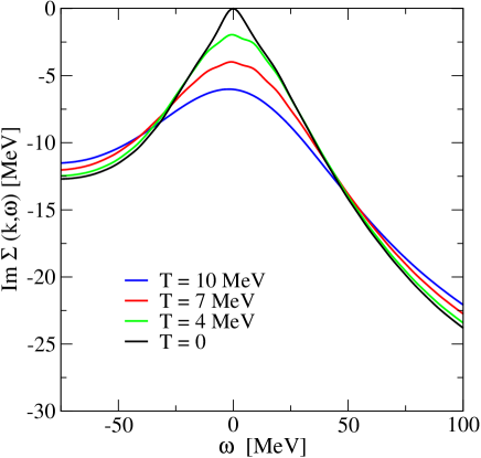
Figure 1: Imaginary part of the retarded self-energy for nucleons with momentum $k$ = 225 MeV/c in symmetric nuclear matter at the empirical saturation density ($\rho$ = 0.16 fm^-3). Results for temperatures $T$ larger than or equal to 4 MeV are directly determined by SCGF calculations, while the $T=0$ result originates from an extrapolation. All results were obtained using the CDBonn interaction.

IV RESULTS AND DISCUSSION

IV.1 SCGF above the critical temperature

In the first part of this section we will focus the attention to the discussion of SCGF calculations for symmetric nuclear matter and pure neutron matter at temperatures above the critical temperature $T_{c}$ for a phase transition to a pairing condensate. This means that we solve Eqs. (12) - (15) in an iterative procedure until a self-consistent solution is obtained. Some details of this procedure have been published in frmu:03 and thesis:fr .

As a typical example we present in Fig. 1 results for the imaginary part of the retarded self-energy $\Sigma(k,\omega)$ for nucleons with a fixed momentum $k$ as a function of the energy variable $\omega$. All the results displayed in this figure have been determined for symmetric nuclear matter at the empirical saturation density using the CDBonn cdbonn interaction. The energy scale in this figure has been constrained to energies around the Fermi energy ($\omega=0$), since the self-energy is most sensitive to the temperature for these energies. The results for temperatures larger than or equal to 4 MeV, which are all above $T_{c}$ (see below), have been obtained directly from SCGF calculations. They exhibit a rather smooth dependence on the temperature, so that an extrapolation to temperatures below $T_{c}$ appears feasible. As an example of such an extrapolation we show the $T=0$ result. This extrapolation has been done with the constraint that the imaginary part of the self-energy for $T=0$ vanishes at $\omega$ =0.

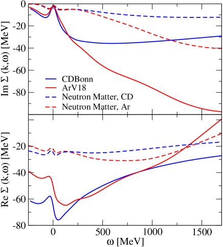
Figure 2: Imaginary (upper panel) and real part (lower panel) of the retarded self-energy for nucleons with momentum $k$ = 225 MeV/c in symmetric nuclear matter at the empirical saturation density ($\rho$ = 0.16 fm^-3). Results obtained for CDBonn interaction are compared to those resulting from SCGF calculations using ArV18. Also included are results for neutrons with the same momentum in neutron matter at $\rho$ = 0.08 fm^-3. The temperature in all these calculations was fixed at $T$=5 MeV.

The imaginary part of the nucleon self-energy is also displayed in the upper panel of Fig. 2. The purpose of this figure is to visualize some differences between various models of the NN interaction and between symmetric nuclear matter and pure neutron matter. Therefore we consider a larger interval for the energy variable $\omega$. The imaginary parts of the self-energy derived from the CDBonn interaction and the Argonne V18 (ArV18) interaction arv18 are very similar at energies around $\omega=0$. At those energies the ArV18 yields a slightly weaker imaginary part than CDBonn. The differences get larger at positive values of $\omega$, where the imaginary part of the self-energy derived from ArV18 reaches a minimum of around -100 MeV at an energy $\omega$ around 1.7 GeV. The minimum for the CDBonn interaction is only about -35 MeV and occurs at energies $\omega$ around 0.5 GeV.

This is another indication of the feature, that a fit of a local interaction, like ArV18, to NN phase shifts yields a larger amount of NN correlations than a fit of a non-local relativistic meson exchange model like the CDBonn fitting identical phase shifts mupo:00 ; gad:01 . In short: The ArV18 is a stiffer interaction than CDBonn. A further illustration is provided by a Hartree-Fock calculation for nuclear matter at the empirical saturation density that yields a total energy 30 MeV per nucleon for the ArV18, while CDBonn generates 5 MeV per nucleon mupo:00 . This implies that the generalized Hartree-Fock contribution to the self-energy in Eq. (7), defined in Eq. (7), is more repulsive for ArV18, and a larger part of the attraction is provided by the energy-dependent contribution to the real part of the self-energy. This is immediately obvious, since the energy-dependent contribution to the real part of $\Sigma$ is connected to the imaginary part by a dispersion relation. The lower panel of Fig. 2, which displays results for the real part of the self-energy, illustrates this observation: The energy dependence is larger for ArV18 as compared to CDBonn. The weaker attraction of the self-energy derived from CDBonn (for most values of $\omega$) reflects the less repulsive contribution of the generalized Hartree-Fock contribution.

Figure 2 also displays results for the real and imaginary part of the self-energy for neutrons with the same momentum ($k$ = 225 MeV) in pure neutron matter. The density of neutron matter considered in this figure is one half of the empirical saturation density of nuclear matter, which implies that these systems have the same Fermi momentum. The imaginary part of the self-energy in neutron matter is weaker than the corresponding one for symmetric nuclear matter, reflecting the dominance of proton-neutron correlations. For both interactions a minimum is obtained around 1.7 GeV. At these high energies the absolute value for the imaginary part of the self-energy is about a factor three larger for ArV18 than for CDBonn. This means that the distribution of sp strength to high energies due to central short-range correlations is much stronger for the local ArV18 interaction than for the non-local meson-exchange model CDBonn. The results for the lower energies are closer to each other. The differences in the amount of NN correlations is also reflected in the occupation probability $n(k)$ defined in (15). For symmetric nuclear matter at saturation density we obtain for $n(k=0)$ the values 0.89 and 0.87 for CDBonn and ArV18, respectively. The corresponding value for neutron matter are $n(k=0)$ = 0.968 and 0.963. Earlier non-self-consistent calculations with older NN interactions tended to yield values of 0.83 for this quantity vond1 in nuclear matter, with self-consistency raising the number to 0.85 rd .

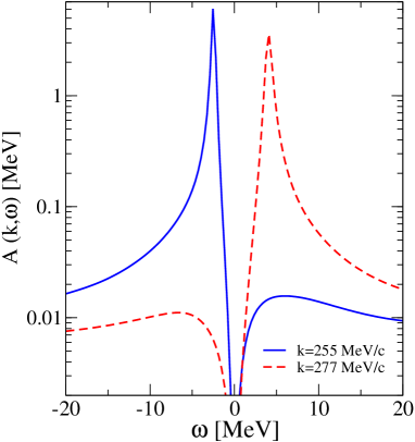
Figure 3: Spectral function for nucleons in symmetric nuclear matter at the empirical saturation density. Results of SCGF calculations have been extrapolated to $T=0$. The CDBonn interaction has been used.

Examples for spectral functions $A(k,\omega)$ are displayed in Fig. 3. Again we consider the case of symmetric nuclear matter at the empirical saturation density and use the CDBonn interaction. As examples we consider two momenta $k=255$ MeV/c and $k=277$ MeV/c, which are below and above the Fermi-momentum $k_{F}$, respectively. For the momentum $k<k_{F}$ one finds the dominant peak at an energy below the Fermi energy $\omega=0$ and a much smaller maximum at $\omega$ larger than zero. For momenta $k>k_{F}$ the dominant quasi-particle peak is located at positive values of $\omega$ and a second maximum occurs at $\omega<0$. Since this feature of two maxima in the spectral function is reminiscent of the two poles that are present in the BCS approximation to the Green’s function, it has been discussed as the formation of a pseudo-gap or as a precursor phenomenon to a pairing condensate boz:99 . We note, however, that our calculations only exhibit this feature of two pronounced maxima in the spectral function, if we consider rather low temperatures, in particular $T<T_{c}$. The examples displayed in Fig. 3 originate from an extrapolation of the self-energy to $T=0$. This is different from results obtained with simplified interactions, as they are used e.g. in Ref. boz:99 . The interaction employed by Bożek yields an imaginary part of the self-energy, which is different from zero in a much smaller energy interval than the realistic calculations considered here. Due to this difference spectral functions with two maxima are obtained also at temperatures above $T_{c}$ for this model interaction.

IV.2 Pairing correlations

As a first step towards the study of pairing correlations, we consider the usual BCS approach. This means that we solve the gap equation (23) assuming a spectrum of sp energies $\varepsilon(k)=\chi_{k}+\mu$, which we determine from the quasi-particle energies

$$\varepsilon(k)=\frac{k^{2}}{2m}+\mathrm{Re}\Sigma(k,\varepsilon(k)-\mu)\,.$$ (25)

In this equation $\mathrm{Re}\Sigma$ denotes the result of a SCGF calculation extrapolated to $T=0$. Such spectra of quasi-particle energies are rather similar to the sp spectra used in other work. The corresponding BCS calculations therefore involve the usual procedure as it has been applied e.g. in Refs. dehj:03 ; ars:90 ; vgdpr:91 ; bbl:92 ; tt:93 ; bls:95 .

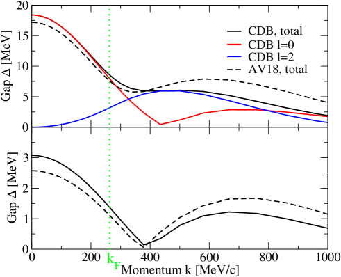
Figure 4: Results for the gap-functions $|\Delta_{l}(k)|$ for symmetric nuclear matter ($\rho$ = 0.16 fm^-3, upper panel) and pure neutron matter ($\rho$ = 0.08 fm^-3, lower panel) obtained from a solution of the BCS equation (23) using the CDBonn and ArV18 interactions at $T=0$. The dotted line identifies the Fermi-momentum $k_{F}$.

Results for the gap-functions $|\Delta_{l}(k)|$ are displayed in Fig. 4. The upper panel of this figure shows results for symmetric nuclear matter at saturation density. The partial wave that yields the largest value for $\Delta$ and is therefore the relevant one in this case, is the ${}^{3}S_{1}-^{3}D_{1}$ channel describing the proton-neutron interaction. We therefore display the absolute values of the gap-functions for $l=0$ and $l=2$ ($\Delta_{0}$ and $\Delta_{2}$) as well as the total gap-function $\Delta=\sqrt{\Delta_{0}^{2}+\Delta_{2}^{2}}$ as a function of the momentum $k$. Below we will mainly consider the value of the gap-function $\Delta$ at the Fermi momentum $k_{F}$. We also compare in this figure the results obtained from CDBonn with those from ArV18. For smaller values of $k$ the CDBonn yields larger values for the gap function, while ArV18 leads to larger gap values for momenta larger than $k=400$ MeV/c. This is true for the $l=0$ component as well as the $l=2$ component and consequently also for the total result. This feature at large values of $k$ is in line with our observation made above, that ArV18 tends to produce a larger amount of correlations at high momenta and large energies. For lower momenta, however, CDBonn yields larger gap-functions. Therefore the gap (at the Fermi momentum) resulting from a BCS calculation, which uses CDBonn (8.6 MeV) is larger than the corresponding value calculated for ArV18 (7.6 MeV), although ArV18 tends to produce more short-range correlations than CDBonn.

The situation is quite similar for the case of neutron-neutron pairing in pure neutron matter, which is displayed in the lower part of Fig. 4. In this case the pairing effects are dominated by the ${}^{1}S_{0}$ partial wave. At high momenta we obtain larger values for the gap function using ArV18, whereas CDBonn yields larger values for $\Delta(k)$ at low momenta. Therefore the value $\Delta(k_{F})$ is larger for CDBonn (1.4 MeV) than for ArV18 (1.1 MeV). These values for the neutron-neutron pairing gap are, however, much lower than the corresponding values for proton-neutron pairing at the same Fermi momentum. On one hand this sounds natural, as we know that the proton-neutron interaction is stronger than the neutron-neutron interaction, leading to a bound deuteron and to more correlations (see above). On the other hand, however, one observes the effects of proton-proton and neutron-neutron pairing in finite nuclei, while there is hardly any trace of proton-neutron pairing effects in nuclei.

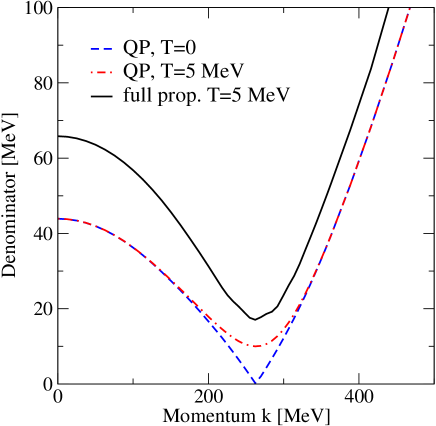
Figure 5: The quantity $\widetilde{\chi}_{k}$ defined in Eq. (26), which represents the energy denominator for the propagator of two nucleons in the medium. Results are displayed for the quasi-particle approximation in the limit $T=0$ (QP, T=0), the quasi-particle approximation for finite temperature $T=5$ MeV (QP, T=5 MeV) and the dressed propagator resulting from SCGF calculations (full prop., T=5 MeV). All results displayed in this figure were obtained for symmetric nuclear matter at density $\rho$ = 0.16 fm^-3, using CDBonn interaction.

As a next step, we now try to consider the effects of temperature and short-range correlations in the solution of the gap equation. For that purpose we will reconsider the two-particle propagator of Eq. (24) but replace the spectral function of the superfluid phase, $A_{s}(k,\omega^{\prime})$, by the corresponding one for the normal phase, $A(k,\omega^{\prime})$. If we consider this propagator in the limit of the mean-field approximation ($A(k,\omega)=\delta(\omega-\varepsilon_{k})$) at $T=0$, it reduces to an energy denominator of the form

$$\frac{1}{-2\widetilde{\chi}_{k}}=:\int_{-\infty}^{+\infty}\frac{{\mathrm{d}}\omega}{2\pi}\int_{-\infty}^{+\infty}\frac{{\mathrm{d}}\omega^{\prime}}{2\pi}A(k,\omega)A(k,\omega^{\prime})\frac{1-f(\omega)-f(\omega^{\prime})}{-\omega-\omega^{\prime}}\quad\stackrel{{\scriptstyle{\rm mf,}T=0}}{{\longrightarrow}}\quad\frac{1}{-2|\chi_{k}|}\,.$$ (26)

This means that the energy $\widetilde{\chi}_{k}$ has been defined in this equation to exhibit the effects of finite temperature and correlations on the two-particle propagator. Figure 5 displays results for this quantity $\widetilde{\chi}_{k}$, the inverse of this propagator multiplied by -2, and compares it with $|\chi_{k}|$ using the corresponding quasi-particle energies. The dashed-dotted line represents the effects of temperature, i.e. the propagator has been calculated using the quasi-particle approach for the spectral function and the Fermi function for the temperature under consideration, while the solid line accounts for finite temperature and correlation effects. The finite temperature yields an enhancement of the effective sp energy $\widetilde{\chi}_{k}$ for momenta around the Fermi-momentum, only. Including in addition the effects of correlations in the propagator, we obtain larger values for $\widetilde{\chi}_{k}$ for all momenta. This corresponds to the well known feature that a finite temperature yields a depletion of the occupation probability of sp states only for momenta just below the Fermi momentum, while strong short-range correlation provide such a depletion for all momenta of the Fermi sea.

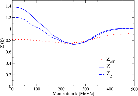
Figure 6: Effective renormalization constants for the sp strength located in the quasi-particle peak as derived from Eq. (27) are compared to the estimates of Eq. (28) and Eq. (29). Further details as in Fig. 5.

Now one may try to describe this depopulation of the sp strength due to the short-range correlations by a factor $Z$, which represents the part of the sp strength contained in the quasi-particle peak. Considering the propagator of Eq. (26) we define

$$\frac{1}{-2\widetilde{\chi}_{k}}(\mbox{T, dressed})=\frac{Z_{eff}^{2}(k)}{-2\chi_{k}}(\mbox{T, QP})\,,$$ (27)

which means that we determine $Z_{eff}$ e.g. from the ratio of the results displayed by the solid and the dashed-dotted line in Fig. 5. Results for such a strength factor are displayed in Fig. 6. Typical values for $Z_{eff}(k)$ are around 0.8 to 0.9 and show only a weak dependence on $k$. This demonstrates that the effects of correlations may be expressed in terms of a renormalization factor $Z(k)$ to be used in the usual BCS equation. Such renormalization effects have been discussed by Bożek boz:03 ; boz:00 and Baldo et al. blsz:02 . Note, however, that the renormalization factor $Z_{eff}(k)$ is defined by Eq. (27) and the complete distribution of sp strength is required to calculate it. It will be interesting to examine, to which extend this factor can be approximated by simpler estimates for the strength located in the quasi-particle peak.

For that purpose we present in Fig. 6 also results from simple estimates of this strength distribution. If one assumes that the imaginary part of the self-energy is a constant, not depending on the energy variable $\omega$, one can estimate this renormalization factor by

$$Z_{1}(k)=\frac{1}{1-\frac{d\mathrm{Re}\Sigma}{d\omega}}\,.$$ (28)

Note, however, that the real-part of the self-energy $\mathrm{Re}\Sigma$ calculated in SCGF yields negative slopes as a function of energy for various momenta and energies (see Fig. 2). Therefore the values for $Z_{1}(k)$ yield values larger than 1 over a wide range of momenta, which is very different from the corresponding values for $Z_{eff}(k)$. One may try to improve the estimate for the strength factor by accounting for an energy dependence of the imaginary part of the self-energy $\mathrm{Im}\Sigma$. This leads to jlm

$$Z_{2}(k)=\frac{1}{\sqrt{\left(1-\frac{d\mathrm{Re}\Sigma}{d\omega}\right)^{2}+\left(\frac{d\mathrm{Im}\Sigma}{d\omega}\right)^{2}}}\,.$$ (29)

This improvement also does not lead to results that are consistent with $Z_{eff}(k)$ (see Fig. 6). This means that we expect results for the generalized gap-equation (20) which are similar to those obtained in Refs. boz:03 ; boz:00 ; blsz:02 using appropriate values for $Z_{eff}(k)$ but we cannot give a simple reliable scheme to estimate the values for the renormalization constants. We therefore determine the dressed two-particle propagator in Eq. (26) within the SCGF approximation by extrapolating the self-energy to temperatures below $T_{c}$, as discussed above. We define an effective sp spectrum according to Eq. (26) and solve the gap equation (23) with this effective sp spectrum.

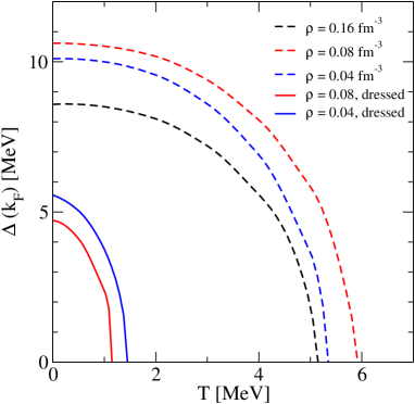
Figure 7: Gap parameter $\Delta(k_{F})$ in symmetric nuclear matter as a function of temperature $T$. Results are presented for various densities, with and without taking into account the dressing of the sp propagator due to short-range correlations. The pairing gap disappears at $\rho$=0.16 fm^-3, if dressed propagators are considered. All results displayed in this figure were obtained using the CDBonn interaction.

Results for the gap parameter $\Delta(k_{F})$ in symmetric nuclear matter of various densities are presented in Fig. 7 as a function of the temperature $T$. We will first discuss the results obtained within the usual BCS approximation (see discussion above) in the ${}^{3}S_{1}-^{3}D_{1}$ partial wave. At the empirical saturation density the CDBonn interaction yields a gap parameter $\Delta(k_{F})$ at temperature $T=0$ of 8.6 MeV (see above), which decreases with increasing temperature until it vanishes at $T=5.2$ MeV. At $\rho$ = 0.08 fm^-3, which is about half the empirical density, the value of the gap parameter at $T=0$ is even larger ($\Delta(k_{F})$ = 10.6 MeV) and the gap calculated within the usual BCS approach disappears only at a temperature of 5.9 MeV. This increase of the pairing gap with decreasing density can be related to the momentum-dependence of the pairing gap $\Delta(k)$ as displayed in Fig. 4: The gap function increases with decreasing momentum. Therefore, as the Fermi momentum decreases with density, the value $\Delta(k_{F})$ tends to decrease with density. At even lower densities, however, this effect is more than compensated by the feature, that the phase-space of two-hole configurations decreases with density, so that ultimately the gap parameter will approach the binding energy of the deuteron in the limit of $\rho\to 0$. This explains the decrease of the gap parameter going from $\rho$ = 0.08 fm^-3 to $\rho$ = 0.04 fm^-3.

If we take the effects of short-range correlations into account, the generalized gap equation of Eq. (20) does not give a non-trivial solution for symmetrical nuclear matter at $\rho$ = 0.16 fm^-3. This means that a proper treatment of correlation effects in nuclear matter at normal density yields a disappearance of the proton-neutron pairing predicted by the usual BCS approach. The effects of short-range correlations tend to decrease with density. As a consequence we obtain non-vanishing gaps for proton-neutron pairing at lower densities (see solid lines in Fig. 7). This also leads to an increase of the critical temperature and the value of $\Delta(k_{F})$ at $T=0$ going from $\rho$ = 0.08 fm^-3 to $\rho$ = 0.04 fm^-3. Note, that these functions are qualitatively different from the corresponding BCS predictions.

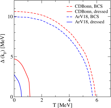
Figure 8: Gap parameter $\Delta(k_{F})$ in symmetric nuclear matter at $\rho$=0.08 fm^-3 as a function of temperature $T$ using the ArV18 and the CDBonn interaction.

Differences associated with the various interactions are displayed in Fig. 8. For nuclear matter with a density of $\rho$ = 0.08 fm^-3 the gap parameter is presented as a function of temperature $T$ using the BCS approximation and the generalized gap equation with dressed propagators. As has already been discussed above, the ArV18 interaction yields smaller values for the gap parameter and the critical temperature than the CDBonn interaction.

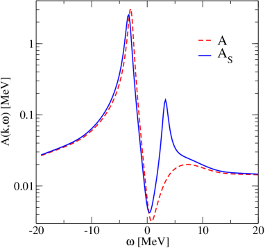
Figure 9: Spectral function for nucleons with momentum $k$ = 193 MeV/c with (solid line) and without (dashed line) inclusion of pairing correlations. Results are presented for nuclear matter of $\rho$ = 0.08 fm^-3 at a temperature $T$ = 0.5 MeV.

Effects of pairing correlations on the spectral function are visualized in Fig. 9. As an example we consider nuclear matter at $\rho$ = 0.08 fm^-3 and show results for the spectral function without ($A(k,\omega)$) and with inclusion of pairing correlations ($A_{s}(k,\omega)$, see Eq. (19)). The momentum considered for this figure, $k$ = 193 MeV/c, is slightly below the Fermi momentum $k_{F}$ = 208 MeV/c. One observes that the inclusion of pairing correlations enhances the maximum of the spectral distribution at positive values of $\omega$ considerably and shifts the quasi-particle peak to more negative values of $\omega$. The pairing correlations modify the spectral distribution into the direction which is obtained in the simple BCS approximation for $A_{s}(k,\omega)$ in Eq. (21). Also note, that these modifications of the spectral function $A_{s}(k,\omega)$ as compared to $A(k,\omega)$ is limited to a small interval of energies around $\omega=0$ and to momenta close to the Fermi momentum.

Finally, we consider the case of neutron-neutron pairing in pure neutron matter. We will focus the attention to densities, where the pairing correlations in the ${}^{1}S_{0}$ partial wave are dominating. Results for the gap parameter $\Delta(k_{F})$ as a function of temperature are displayed in Fig. 10. Using the BCS approximation with sp energies derived from the quasi-particle energies of SCGF calculations we obtain a gap at $T=0$, which, for the range of densities considered, increases with decreasing density. This is in agreement with results of similar calculations, which are summarized e.g. in dehj:03 .

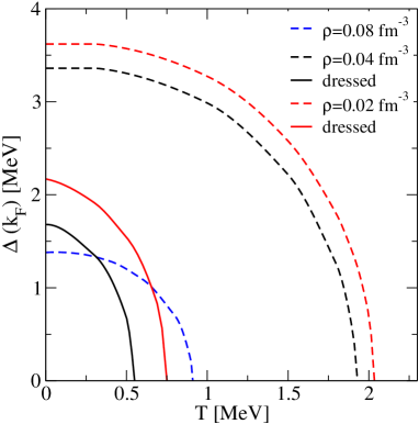
Figure 10: Gap parameter $\Delta(k_{F})$ in neutron matter as a function of temperature $T$. Results are presented for the usual BCS approximation (dashed lines) and the solution of the generalized gap equation (20) in the ${}^{1}S_{0}$ partial wave using the CDBonn interaction.

The effects of short-range correlations are weaker in neutron matter than in nuclear matter. This has been discussed already above in connection with the results displayed in Fig. 2. This can also be seen in a comparison of the dressed two-particle propagator and the effective strength factor $Z_{eff}$ defined in Eq. (27). While a calculation of $Z_{eff}$ for symmetric nuclear matter at $\rho$ = 0.16 fm^-3 yields values for $Z_{eff}$, which are typically around 0.8 (see Fig. 6), corresponding values for $Z_{eff}$ in neutron matter at $\rho$ = 0.08 fm^-3 are around 0.9. Nevertheless, also these weaker effects of short-range correlations in neutron matter are sufficient to suppress the formation of a pairing gap in neutron matter at $\rho$ = 0.08 fm^-3. Such a suppression of pairing correlations is also observed at smaller densities. In this case, however, the inclusion of the correlation effects just leads to a reduction of the gap parameter at a given temperature and a reduction of the critical temperature (see Fig. 10). Extrapolating our results to neutron matter with higher densities, we expect that the short-range correlations will suppress the formation of pairing in the ${}^{3}P_{2}-^{3}F_{2}$ partial waves at those densities khcl .

V CONCLUSIONS

An attempt has been made to treat the effects of short-range and pairing correlations in a consistent way within the $T$-matrix approach of the self-consistent Green’s function (SCGF) method. The pairing effects are determined from a generalized gap equation that employs sp propagators fully dressed by short-range and tensor correlations. This equation is directly linked to the homogeneous solution of the $T$-matrix equation of NN scattering in the medium, which is one of the basic equations of the SCGF approach at temperatures above the critical temperature for a phase transition to pairing condensation. While short-range and tensor correlations yield a redistribution of sp strength over a wide range of energies, the effects of pairing correlations on the spectral function are limited in nuclear matter to a relatively small interval in energy and momentum around the Fermi surface.

The formation of a pairing gap is very sensitive to the quasi-particle energies and strength distribution at the Fermi surface and can be suppressed by moderate temperatures. The formation of short-range correlations are sensitive to a larger range of energies and momenta. So we observe, that the non-local CDBonn interaction is softer with respect to the formation of short-range correlations but yields larger pairing gaps compared to the local ArV18 model for the NN interaction.

From this sensitivity to different areas in momentum and energy one may conclude that the features of short-range correlations should be rather similar in studies of nuclear matter and finite nuclei. The investigation of pairing phenomena, however, is rather sensitive e.g. to the energy spectrum around the Fermi energy. Therefore the shell effects of finite nuclei may lead to quite different results for pairing properties than corresponding studies in infinite matter.

The redistribution of sp strength due to the short-range correlations has a significant effect on the formation of a pairing gap. While the usual BCS approach predicts a gap for proton-neutron pairing in nuclear matter at saturation density as large as 8 MeV, the inclusion of short-range correlations suppresses this gap completely. Correlation effects are weaker at smaller densities, but still lead to a significant quenching of the proton-neutron pairing gap and to a reduction of the critical temperature for the phase transition. Compared to symmetric nuclear matter correlation effects are weaker in neutron matter. Nevertheless, the inclusion of correlations suppresses the formation of a gap for neutron-neutron pairing at $\rho$ = 0.08 fm^-3 completely and yields a significant quenching at lower densities.

The effects of dressed sp propagator in the generalized gap equation could be described in terms of an effective strength factor $Z_{e}ff{k}$, which has been considered in the literature before boz:03 ; boz:00 ; blsz:02 . Unfortunately, we have not been able to derive the value of this strength factor from bulk properties of the self-energy.

Although the effects of pairing correlations on the sp Green’s function is weak and limited to a small range in energy and momentum, these modifications are very important to extend SCGF calculations to densities and temperatures that suffer from the so-called pairing instability. The present study is a first step towards a consistent treatment of pairing and short-range correlations.

This work is supported by the U.S. National Science Foundation under Grant No. PHY-0140316 and the “Landesforschungsschwerpunkt Quasiteilchen” of the state of Baden Württemberg. H.M. would like for the hospitality of the Department of Physics of Washington University in St. Louis, where a major part of this work has been done.

References

- (1) W.H. Dickhoff and C. Barbieri, Prog. Nucl. Part. Phys. 52, 377 (2004).
- (2) M.F. van Batenburg, Ph.D. Thesis, University of Utrecht (2001).
- (3) B.E. Vonderfecht, W.H. Dickhoff, A. Polls, and A. Ramos, Phys. Rev. C 44, R1265 (1991).
- (4) D. Rohe, et al., Phys. Rev. Lett. 93, 182501 (2004).
- (5) H. Müther and W.H. Dickhoff, Phys. Rev. C 49, R17 (1994).
- (6) T. Frick and H. Müther, Phys. Rev. C 68, 034310 (2003).
- (7) T. Frick, Ph.D. Thesis, University of Tübingen (2004).
- (8) B.E. Vonderfecht, W.H. Dickhoff, A. Polls, and A. Ramos, Nucl. Phys. A555, 1 (1993).
- (9) D.J. Dean and M. Hjorth-Jensen, Rev. Mod. Phys. 75, 607 (2003).
- (10) Q. Chen, J. Stajic, S. Tan, and K. Levin, Phys. Rep. 412, 1 (2005).
- (11) D. Blaschke, H. Grigorian, and D.N. Voskresensky, Astron. Astrophys. 424, 979 (2004).
- (12) T. Alm, G. Röpke, and M. Schmidt, Z. Phys. A 337, 355 (1990).
- (13) B.E. Vonderfecht, C.C. Gearhart, W.H. Dickhoff, A. Polls, and A. Ramos, Phys. Lett. B 253, 1 (1991).
- (14) M. Baldo, I. Bombaci, and U. Lombardo, Phys. Lett. B 283, 8 (1992).
- (15) T. Takatsuka and R. Tamagaki, Suppl. Prog. Theor. Phys. 112, 27 (1993).
- (16) M. Baldo, U. Lombardo, and P. Schuck, Phys. Rev. C 52, 975 (1995).
- (17) W. Zuo, U. Lombardo, H.-J. Schulze, and C.W. Shen, Phys. Rev. C 66, 037303 (2002).
- (18) A. Sedrakian, Phys. Rev. C 68, 065805 (2003).
- (19) Caiwan Shen, U. Lombardo, P. Schuck, W. Zuo, and N. Sandulescu, Phys. Rev. C 67, 061302 (2003).
- (20) Caiwan Shen, U. Lombardo, and P. Schuck, Phys. Rev. C 71, 054301 (2005).
- (21) J. Decharge and D. Gogny, Phys. Rev. C 21, 1568 (1980).
- (22) W.H. Dickhoff and H. Müther, Nucl. Phys. A 473, 394 (1987).
- (23) R.B. Wiringa, V.G.J. Stoks, and R. Schiavilla, Phys. Rev. C 51, 38 (1995).
- (24) R. Machleidt, F. Sammarruca, and Y. Song, Phys. Rev. C 53, R1483 (1996).
- (25) W. H. Dickhoff and E. P. Roth, Acta Phys. Pol. B 33, 65 (2002); E. P. Roth, Ph.D. thesis Washington University, St. Louis (2000).
- (26) Y. Dewulf, D. Van Neck, and M. Waroquier, Phys. Rev. C 65, 054316 (2002).
- (27) P. Bożek and P. Czerski, Eur. Phys. J. A 11, 271 (2001).
- (28) P. Bożek, Phys. Rev. C 65, 054306 (2002).
- (29) P. Bożek, Eur. Phys. J. A 15, 325 (2002).
- (30) Y. Dewulf, W.H. Dickhoff,D. Van Neck, E.R. Stoddard, and M. Waroquier, Phys. Rev. Lett 90, 152501 (2003).
- (31) A.E.L. Dieperink, Y. Dewulf, D. Van Neck, and M. Waroquier, Phys. Rev. C 68, 064307 (2003).
- (32) T. Frick, H. Müther, A. Rios, A. Polls, and A. Ramos, Phys. Rev. C 71, 014313 (2005).
- (33) A. Schnell, G. Röpke, and P. Schuck, Phys. Rev. Lett. 83, 1926 (1999).
- (34) P. Bożek, Nucl. Phys. A 657, 187 (1999).
- (35) P. Bożek, Phys. Lett. B 551, 93 (2003).
- (36) W.H. Dickhoff, C.C. Gearhart, E.P. Roth, A. Polls, and A. Ramos, Phys. Rev. C 60, 064319 (1999).
- (37) M. Baldo and A. Grasso, Phys. Lett. B 485, 115 (2000).
- (38) U. Lombardo, P. Schuck, and W. Zuo, Phys. Rev C 64, 021301(R) (2001).
- (39) M. Baldo, U. Lombardo, H.-J. Schulze, and Zuo Wei, Phys. Rev C 66, 054304 (2002).
- (40) L. P. Kadanoff and G. Baym, Quantum Statistical Mechanics (Benjamin, New York, 1962)
- (41) T. Alm, B. L. Friman, G. Röpke and H. Schulz, Nucl. Phys. A 551, 45 (1993).
- (42) T. Alm, G. Röpke, A. Schnell, N.H. Kwong, and H.S. Köhler, Phys. Rev. C 53, 2181 (1995).
- (43) E. Schiller, H. Müther, and P. Czerski, Phys. Rev. C 59, 2934 (1999).
- (44) A.B. Migdal, Theory of Finite Fermi Systems (Wiley, New York, 1967).
- (45) J.R. Schrieffer, Theory of Superconductivity (Benjamin, Massachusetts, 1964).
- (46) G.D. Mahan, Many-Particle Physics (Plenum Press, New York, 1981).
- (47) W.H. Dickhoff and D. Van Neck, Many-Body Theory Exposed! (World Scientific, Singapore, 2005).
- (48) T. Frick, Ph.D. Thesis, University of Tübingen, (2004).
- (49) H. Müther and A. Polls, Prog. Part. and Nucl. Phys. 45, 243 (2000).
- (50) T. Frick, Kh. Gad, H. Müther, and P. Czerski, Phys. Rev. C 65, 34321 (2002).
- (51) P. Bożek, Phys. Rev. C 62, 054316 (2000).
- (52) J.P. Jeukenne, A. Lejeune, and C. Mahaux, Phys. Rep. 25, 83 (1976).
- (53) V.A. Khodel, V.V. Khodel, and J.W. Clark, Phys. Rev. Lett. 81, 3828 (1998).