The Piecewise Moments Method: A Generalized Lanczos Technique for Nuclear Response Surfaces

Abstract

For some years Lanczos moments methods have been combined with large-scale shell-model calculations in evaluations of the spectral distributions of certain operators. This technique is of great value because the alternative, a state-by-state summation over final states, is generally not feasible. The most celebrated application is to the Gamow-Teller operator, which governs $\beta$ decay and neutrino reactions in the allowed limit. The Lanczos procedure determines the nuclear response along a line $q$=0 in the $(\omega,q)$ plane, where $\omega$ and $q$ are the energy and three-momentum transfered to the nucleus. However, generalizing such treatments from the allowed limit to general electroweak response functions at arbitrary momentum transfers seems considerably more difficult: the response function must be determined over the entire $(\omega,q)$ plane for an operator $O(q)$ that is not fixed, but depends explicitly on $q$. Such operators arise in any semileptonic process where the momentum transfer is comparable to (or larger than) the inverse nuclear size. Here we show, for Slater determinants built on harmonic oscillator basis functions, that the nuclear response for any multipole operator $O(q)$ can be determined efficiently over the full response plane by a generalization of the standard Lanczos moments method. We describe the Piecewise Moments Method and thoroughly explore its convergence properties for the test case of electromagnetic responses in a full $sd$-shell calculation of ²⁸Si. We discuss possible extensions to a variety of electroweak processes, including charged- and neutral-current neutrino scattering.

I Introduction and Motivation

The shell model caur is an important tool for modeling the ground states and low-lying excitations of nuclei, as well as their electromagnetic and weak-interaction properties. Calculations are performed by diagonalizing an effective interaction $H$ within a low-momentum model space typically consisting of all Slater determinants that can be constructed within one or perhaps a few principal shells. $H$ corrects for the absence of the remaining shells and of the high-momentum correlations that reside primarily in those excluded shells. Typically $H$ is determined empirically brown , though recently considerable work has been invested in various effective-theory approaches to derive $H$ directly from the underlying bare interaction song .

With increasing CPU speeds and the advent of parallel computing, shell model practitioners have been able to tackle problems in very large bases – ranging in some cases to Hamiltonians of dimension $\sim 10^{8}-10^{9}$ caur . Because direct diagonalizations in such spaces are impossible, iterative methods are used to determine extremum eigenvalues and their eigenfunctions. The Lanczos algorithm lanczos is the most commonly used method. It is based on a recursive mapping of the full Hamiltonian into a much smaller, tridiagonal matrix that preserves certain exact information on the lowest moments of the full Hamiltonian. As described in the next section, extremum eigenvalues of the Lanczos matrix converge to those of the full Hamiltonian because of the algorithm’s moments properties, thus making the algorithm useful as a diagonalization tool. However, its real power is connected with another property, a stable method for solving the classical moments problem – determining the simplest discrete distribution characterized by those same lowest moments.

One can argue that the Lanczos algorithm adresses both of the most common challenges encountered in nuclear structure physics – detailed information about specific low-lying states and global information on spectral moments important to inclusive properties, such as response functions, polarizabilities, and Green’s functions.

The moments method, described in more detail in the next section, can be applied in a straight-forward way to operators like the Gamow-Teller (GT) operator,

$$\sum_{i=1}^{A}\sigma(i)\tau_{\pm}(i).$$

This operator is independent of the three-momentum transfer $q$. GT strength distributions (and their neutral-current analogs) govern low-energy neutrino reactions important to solar and supernova physics. The combination of increasingly sophisticated shell-model ground-state wave functions and Lanczos methods for strength distributions has had great impact. Results include much better agreement between theory and experiment (e.g., $(p,n)$ mappings of GT distributions) and new iron-group weak interaction rates langanke00 that have influenced the collapse and explosion physics of Type II supernovae heger01 ; hix03 .

However, the restriction to allowed operators is very limiting. For example, in supernova physics, approximately half of the strength for heavy-flavor neutral current scattering is carried by momentum-dependent operators haxton88 . Because no efficient moments method is available for these more complex operators, and because state-by-state summations would be prohibitively difficult, theorists have not been able to make use of state-of-the-art shell model wave functions in evaluating inclusive forbidden response functions. Instead less sophisticated methods – simplified shell model treatments, QRPA, or even schematic approaches like the Goldhaber-Teller model – have been substituted, as the resulting smaller Hilbert spaces do allow state-by-state summations. The difficulty in designing a moments method for a multipole operator $O(q)$ that varies with $q$ is clear: the standard moments method would require one to repeat the calculation many times over a grid in $q$, as $O(q)$ is a fixed operator only along $q$=constant trajectories. Furthermore, as will become clearer below, a rather dense grid in $q$ would be needed to interpret an experiment that maps out some nontrivial trajectory in the $(\omega,q)$ response plane, as the discreteness of the moments distributions at each $q$ makes it complicated to extrapolate in $q$.

Interest in general electroweak response functions is not limited to supernova physics, clearly. An electron scattering experiment, for example, generally maps out some area within the space-like half of the response plane, depending on the range of spectrometer angles and electron energy loss explored.

In this paper we show that there is an efficient moments technique for constructing the entire shell-model inclusive response surface – the response $S(\omega,q)$ as a continuous function of both $q$ and $\omega$, as well as of the oscillator parameter $b$ – provided the underlying single-particle basis wave functions are taken to be harmonic oscillators. The method involves a small number of Lanczos calculations (at most three in the ²⁸Si test case we use here). That is, the full response surface can be reconstructed with little more effort than required in the familiar GT case, where results are obtained only for a line $q$=0 in the response plane. The information that must be extracted from the many-body calculations to perform this reconstruction are the elements of the tridiagonal Lanczos matrices and certain dot products between Lanczos vectors. The method can be viewed as a nearly perfect “numerical effective theory,” as it extracts from potentially quite complicated microscopic calculations precisely that information necessary to reconstruct the response surface up to a specified resolution in energy. This has implications for problems like modeling supernova explosions, where one issue in the use of sophisticated nuclear physics results is defining a practical scheme for making the information available “on line” within the explosion codes.

The outline of this paper is as follows: In the next section we review in more detail the Lanczos method, including its conventional uses in constructing response functions and Green’s functions. In the third section we discuss the problem at hand, the construction of response functions for electroweak nuclear operators at arbitrary $(\omega,q)$. We discuss properties of harmonic oscillator matrix elements of these operators which could lead to efficient algorithms for constructing the full response surface. We describe numerical limitations to some possible approaches. In the fourth section we describe the Piecewise Moments Method (PMM), which we formulate first for a Lorentzian resolution function in energy, but then generalize for any choice. In the fifth section we explore convergence properties of the PMM, using as a test case the electromagnetic response functions for a full $sd$-shell calculation of ²⁸Si. Convergence properties of the method are explored and various numerical comparisons are made with “exact” results. A series of results for response surfaces are presented. In the concluding section we discuss opportunities for applying the method, including supernova physics and the neutrino reactions at energies below 1 GeV (e.g., LSND or atmospheric neutrinos). We suggest extensions of the work – to check unitarity and to project spurious states – that might be important in future applications of the PMM.

II Lanczos Algorithm Preliminaries

The Lanczos method is based on a mapping of a Hamiltonian $H$ of dimension $N$ to tridiagonal form by a recursive definition of a new orthonormal basis $|v_{i}\rangle$, called the Lanczos vectors. One begins with an arbitrary unit vector $|v_{1}\rangle$ and performs the successive operations to define the $|v_{i}\rangle$,

$$H|v_{1}\rangle= \alpha_{1}|v_{1}\rangle+\beta_{1}|v_{2}\rangle$$

$$H|v_{2}\rangle= \beta_{1}|v_{1}\rangle+\alpha_{2}|v_{2}\rangle+\beta_{2}|v_{3}\rangle$$

$$H|v_{3}\rangle= \beta_{2}|v_{2}\rangle+\alpha_{3}|v_{3}\rangle+\beta_{3}|v_{4}\rangle$$

$$H|v_{i}\rangle= \beta_{i-1}|v_{i-1}\rangle+\alpha_{i}|v_{i}\rangle+\beta_{i}|v_{i+1}\rangle.$$ (1)

where in the first step $\alpha_{1}|v_{1}\rangle$ is the projection of $H|v_{1}\rangle$ onto $|v_{1}\rangle$, while the remaining orthogonal portion defines a new unit vector and amplitude $\beta_{1}|v_{2}\rangle$. In the third step we see the tridiagonal form emerge, as the construction demands $\langle v_{3}|H|v_{1}\rangle$ = 0. The hermiticity of $H$ has been used above. In practice this algorithm, when used to determine extremum eigenvalues and eigenvectors, is usually executed with a reorthogonalization step in each iteration, to guarantee that the new vector $|v_{i}\rangle$ is orthogonal to all previous vectors. While this step is not required mathematically, it is nevertheless important numerically, as roundoff error can grow with successive iterations cullum85 , eventually leading to a Lanczos matrix that contains multiple copies of subspaces of $H$.

Clearly, if the procedure were continued $N$ steps, one would find $\beta_{N}$ =0, as exhaustion of the Hilbert space terminates the construction. The effect of the Lanczos procedure would be a unitary transformation to a new basis in which the Hamiltonian is tridiagonal, but still of dimension $N$. However, in useful applications $N$ is very large, and the Lanczos construction is truncated by choice after $n$ iterations by setting $\beta_{n}=0$, $n\ll N$. This yields the truncated tridiagonal Lanczos matrix $L(n,|v_{1}\rangle)$

$$L(n,|v_{1}\rangle)=\left(\begin{array}[]{cccccc}\alpha_{1}&\beta_{1}&0&0&&\\ \beta_{1}&\alpha_{2}&\beta_{2}&0&&\cdots\\ 0&\beta_{2}&\alpha_{3}&\beta_{3}&&\\ 0&0&\beta_{3}&\alpha_{4}&&\\ &&\vdots&&\ddots&\\ &&&&\beta_{n-1}&\alpha_{n}\\ \end{array}\right)$$ (2)

The notation emphasizes that $L$ is entirely determined by the number of iterations $n$ and by the choice of the starting vector $|v_{1}\rangle$.

The powerful property of this mapping of $H$ onto a much smaller subspace is that it extracts specific exact information from the full Hamiltonian

$$H(N)\rightarrow L(n,|v_{1}\rangle)$$ (3)

$$\{\langle v_{1}|H^{\lambda}|v_{1}\rangle,\lambda=1,\ldots,2n-1\}\leftrightarrow$$

$$\{\alpha_{1},\ldots,\alpha_{n};\beta_{1},...,\beta_{n-1}\}$$ .

That is, the first $2n-1$ moments of H for the starting vector $|v_{1}\rangle$ determine $L(n,|v_{1}\rangle)$, and conversely. In a very real sense, the Lanczos algorithm can be considered a numerical effective theory. It systematically extracts from the large matrix the long-wavelength information describing the distribution of $|v_{1}\rangle$ over the eigenspectrum of $H$, while leaving behind the high frequency information important to the detailed structure of this distribution, but not to any of its broad features. More precisely, if we denote by $\{(\psi_{E_{i}},E_{i}),i=1,\ldots,N\}$ the exact eigenenergies/functions of $H$ and by $\{(\hat{\psi}_{\hat{E}_{i}},\hat{E}_{i}),i=1,\ldots,n\}$ the eigenenergies/functions of $L(n,|v_{1}\rangle)$, then

$$\langle v_{1}|H^{\lambda}|v_{1}\rangle = \sum_{i=1}^{N}|\langle v_{1}|\psi_{E_{i}}\rangle|^{2}E_{i}^{\lambda}$$ (4)

$$= \sum_{i=1}^{n}|\langle v_{1}|\hat{\psi}_{\hat{E}_{i}}\rangle|^{2}\hat{E}_{i}^{\lambda}$$

$$= \sum_{i=1}^{n}|\hat{\psi}_{\hat{E}_{i}}(1)|^{2}\hat{E}_{i}^{\lambda},\lambda=1,\ldots,2n-1$$

That is, the eigenvalues and eigenvectors of the Lanczos matrix $L(n,|v_{1}\rangle)$ determines a set of $n$ points $\hat{E}_{i}$ and weights that solves the classical moments problem – a discrete distribution whose moments reproduce those of the full matrix $H$. The weights are simply the squares of the first components of the respective Lanczos eigenvectors. As Whitehead has emphased whit1 ; whit2 , the speed and numerical stability of this classical moments solution is a very special property of the Lanczos algorithm.

The usual application of the Lanczos algorithm is in determining extremum eigenvalues, especially the ground state and first few excited states. After each iteration $L(n,|v_{1}\rangle)$ can be diagonalized by standard techniques, determining eigenvalues and eigenfunctions. Because extremum eigenvalues are heavily weighted in $H^{n}$ when $n$ is large and often separated by gaps from the bulk of spectrum, these eigenvalues of $L$ must quickly converge to the true eigenvalues of $H$. This convergence can be monitored numerically as the algorithm is executed. In typical shell model applications the ground state often converges in about 50 iterations, while the lowest 10 or so eigenvalues and eigenfunctions may be resolved in 200 iterations whit2 .

But perhaps the most elegant applications of the Lanczos algorithm are in distribution functions or Green’s functions, inclusive quantities that depend most directly on spectral moments, the long-wavelength information extracted from $H$. Consider the response function $S(\omega)$

$$S(\omega)=\sum_{i=1}^{N}|\langle\psi_{E_{i}}|O|g.s.\rangle|^{2}\delta(\omega-E_{i})$$ (5)

where the sum extends over a complete set of states $i$ of the full Hamiltonian $H$. Assume for the moment that $O$ is a fixed operator, like the Gamow-Teller operator, independent of the three-momentum transfer $q$ to the nucleus. We define a unit vector $|v_{1}\rangle$ by

$$O|g.s.\rangle\equiv c|v_{1}\rangle,$$ (6)

where $c$ is the overall strength (norm). Taking $|v_{1}\rangle$ as the starting vector and competing $n$ Lanczos iterations, one can form the distribution

$$\hat{S}_{n}(\omega)=|c|^{2}\sum_{i=1}^{n}\delta(\omega-\hat{E}_{i})|\hat{\psi}_{\hat{E}_{i}}(1)|^{2}.$$ (7)

If one weights this distribution with $\omega^{\lambda}$ and integrates over $\omega$, one sees from Eq. 4 that $S_{n}(\omega)$ reproduces the lowest $2n-1$ integrated moments of the exact spectral distribution $S(\omega)$.

Now, as experiments are done with finite resolution, spectral variations occurring at energy scales below that resolution are irrelevant. Furthermore, the discrete spectrum of the shell model is itself an artifact of the use of a finite Hilbert space. It represents resonances in the continuum by discrete doorway states, with the density of such states increasing as the shell-model space is expanded, to better represent the continuum. Thus one quickly recognizes that the high-frequency information missing from Eq. 7 may be irrelevant when comparing with experiment. It is customary to replace the $\delta$-function in the Lanczos strength distribution with a resolution function, choosing a width parameter $\sigma$ appropriate to the experiment in question

$$\hat{S}_{n}(\omega,\sigma)=c^{2}\sum_{i}^{n}R(\omega-\hat{E}_{i},\sigma)|\hat{\psi}_{\hat{E}_{i}}(1)|^{2}.$$ (8)

where $R$ is normalized to 1. Common choices are Lorentzians and Gaussians, e.g.,

$$R_{L}(\omega-\hat{E}_{i},\sigma) = {\sigma\over\pi}{1\over(\omega-\hat{E}_{i})^{2}+\sigma^{2}}$$

$$R_{G}(\omega-\hat{E}_{i},\sigma) = {1\over\sigma\sqrt{2\pi}}\exp{(-(\omega-\hat{E}_{i})^{2}/2\sigma)}$$ (9)

Because such smoothing makes high-frequency information irrelevant, the Lanczos approximation $\hat{S}_{n}(\omega,\sigma)$ converges to the exact smoothed distribution $S(\omega,\sigma)$ for $n$ sufficiently large. Qualitatively, convergence is achieved when the typical separation in energy of neighboring Lanczos eigenvectors becomes substantially smaller than the chosen resolution $\sigma$. For $\sigma\sim 0.25$ MeV, a value typical of (p,n) mappings of GT strength, for instance, this may occur at $n\sim 200$. Thus the Lanczos algorithm provides an exact method for determining appropriately smoothed strength functions in very complex shell-model spaces.

A second spectral application is to Green’s functions haydock , which arise in nuclear calculations of polarizabilities, in virtual processes like double $\beta$ decay, and in a variety of many-body applications, such as effective interactions and operators. The Green’s function acting on a normalized vector $|v_{1}\rangle$

$$G(\omega)|v_{1}\rangle={1\over\omega-H}|v_{1}\rangle$$ (10)

can be approximated after $n$ Lanczos iterations as

$$\hat{G}_{n}(\omega)|v_{1}\rangle=\hat{g}_{1}(\omega)|v_{1}\rangle+\hat{g}_{2}(\omega)|v_{2}\rangle+\cdots+\hat{g}_{n}(\omega)|v_{n}\rangle$$ (11)

where the coefficients $\hat{g}_{i}(\omega)$ are finite continued fractions formed from the entries in the tridiagonal matrix. For example

$$\hat{g}_{1}(\omega) = {1\over\omega-\alpha_{1}-{\beta_{1}^{2}\over\omega-\alpha_{2}-{\beta_{2}^{2}\over\omega-\alpha_{3}-\beta_{3}^{2}}}}$$ (12)

$$~{}~{}~{}~{}~{}~{}~{}~{}~{}~{}~{}~{}~{}~{}~{}~{}~{}~{}~{}~{}~{}~{}~{}~{}~{}~{}~{}~{}~{}~{}~{}~{}~{}~{}~{}~{}~{}\ddots$$

With each additional iteration, one additional Lanczos vector is added to the expansion, and each continued fraction increases in rank by one through the addition of a new $\alpha_{n+1}$ and $\beta_{n}$. As most Green’s function applications involve convolutions with relatively smooth operators, often $\hat{G}_{n}(\omega)|v_{1}\rangle$ becomes numerically equivalent to $G(\omega)|v_{1}\rangle$ after a few Lanczos iterations ($\sim$ 20) engel .

An important consequence of Eq. 11 is that, once the Lanczos calculation is completed, the Green’s function is known as a function of $\omega$. This will be important in the applications we discuss later.

III Electroweak Response Functions at Arbitrary $q^{2}$

The discussion of the previous section addressed the special case of a fixed operator, like the GT operator, which governs the weak nuclear response along the $q$=0 line in the $(\omega,q)$ response plane. However many electroweak processes of interest – intermediate-energy electron or neutrino scattering, muon capture, etc. – involve appreciable three-momentum transfers (and the associated excitation of radial modes in the nucleus). That is, the relevant response function is

$$S(\omega,q)=\sum_{i=1}^{N}|\langle\psi_{E_{i}}|O(q)|g.s.\rangle|^{2}\delta(\omega-E_{i})$$ (13)

where $O(q)$ is (an assumed one-body) electroweak operator that depends explicitly on $q$. If one naively applies the formalism of the preceding section, a new calculation would be needed for each desired $q$, because the operator evolves with $q$. This would require tediously stepping over a grid of fixed $q$s, computing a Lanczos calculation for each value, to map the full surface above the response plane.

Here we discuss procedures for evaluating $S(\omega,q)$ very efficiently as a function of $q$ (and $\omega$) over the entire response plane, at the cost of only a few Lanczos calculations. The approach depends on the assumption that the shell-model basis of Slater determinants has been formed from harmonic oscillator single-particle wave functions. This choice allows one to exploit attractive properties of the matrix elements of $O(q)$ between such wave functions.

While we will delay details of the test application (electromagnetic response functions for ²⁸Si) to the next section, here we sketch the basic idea. One can write $O(q)|g.s.\rangle$ in second quantization

$$\sum_{\alpha,\beta}\langle\alpha|O(q)|\beta\rangle a_{\alpha}^{\dagger}a_{\beta}|g.s.\rangle.$$ (14)

where $\alpha$ and $\beta$ represent a complete set of single-particle quantum numbers. For the choice of harmonic oscillators, matrix elements of the standard charge, longitudinal, transverse electric, and transverse magnetic multipoles can be evaluated in closed form, leading to walecka ; donnelly

$$\langle\alpha|O_{J}(q)|\beta\rangle=y^{(J-K)/2}e^{-y}p^{\alpha\beta}(y).$$ (15)

Here we have denoted the multipolarity of the operator by J, K=2(1) for normal(abnormal) parity operators, and $y=(qb/2)^{2}$ with $b$ the oscillator parameter. The crucial point is that $p(y)$ is a finite polynomial in $y$ or $q^{2}$. In the ²⁸Si test case, the most complicated operator that arises has only three nonzero terms in $p(y)$.

We first go through a schematic argument to show how this $y$ dependence might be exploited. Denoting the order of the polynomial $p$ by $m$, it follows that

$$O(q)|g.s.\rangle=$$

$$y^{(J-K)/2}e^{-y}[c_{0}|v_{1}^{0}\rangle+c_{1}y|v_{1}^{1}\rangle+\cdots+c_{m}y^{m}|v_{1}^{m}\rangle]~{}~{}~{}~{}~{}$$

$$\equiv y^{(J-K)/2}e^{-y}c(y)|v_{1}(y)\rangle$$ (16)

using a notation analogous to Eq. 6, with the strength $c_{j}$ chosen to make $|v_{1}^{j}\rangle$ a unit vector. For parity-conserving interactions and standard phase conventions, all quantities can be taken as real, with the $c$s nonnegative. The $|v_{1}^{j}\rangle$, of course, are not orthonormal. Similarly $c(y)$ and $|v_{1}(y)\rangle$ can be viewed as a $y$-dependent strength and unit vector. It follows that

$$S(\omega,q)=y^{J-K}e^{-2y}|c(y)|^{2}\sum_{i=1}^{N}|\langle\psi_{E_{i}}|v_{1}(y)\rangle|^{2}\delta(\omega-E_{i})$$ (17)

where

$$|c(y)|^{2}|\langle\psi_{E_{i}}|v_{1}(y)\rangle|^{2}=\sum_{j,k=0}^{m}c_{k}^{*}c_{j}y^{j+k}\langle v_{1}^{k}|\psi_{E_{i}}\rangle\langle\psi_{E_{i}}|v_{1}^{j}\rangle,$$ (18)

so that the response function has a similar polynomial form. It also follows that moments of $S(\omega)$ have the form

$$\int_{0}^{\infty}S(\omega)\omega^{\lambda}d\omega=y^{J-K}e^{-2y}|c(y)|^{2}\sum_{i=1}^{N}|\langle\psi_{E_{i}}|v_{1}(y)\rangle|^{2}E_{i}^{\lambda}.$$ (19)

These last two results simply state that if one had a complete set of $N$ eigenvalues and eigenfunctions, each contributing transition probability would have a simple, analytical behavior in $y$.

Of course, these results are only of academic interest: as we are assuming $N$ is prohibitively large, a complete diagonalization is impossible. This leaves a much more interesting question: can we find an analog of Eq. 7 or 8, an efficient Lanczos representation of $S(\omega,q)$, that also exploits the polynomial behavior of the response in $y$? If so, it would appear to be a practical way to construct the response over the entire $(\omega,q)$ plane.

We have explored several of the possibilities, uncovering some of the numerical pitfalls. Even the less successful methods are interesting conceptually, so we describe the approaches qualitatively below, reserving details for the Appendix. Finally, we describe and test the Piecewise Moments Method, demonstrating that it is effectively exact and stable for an arbitrary number of iterations.

The Naive Moments Method: The most straightforward approach to the above problem exploits the equivalence between the tridiagonal matrix $L(n,|v_{1}(y)\rangle)$ and the moments $\langle v_{1}(y)|H^{\lambda}|v_{1}(y)\rangle,\lambda=1,\dots,2n-1$. If we had a method to determine $L(n,|v_{1}(y)\rangle)$ as a continuous function of $y$, Eq. 7 could be then be used at any $y$. The result would be a discrete distribution along any line $y$=constant, that would evolve smoothly as $y$ is changed.

The moments equivalence shows this is possible as

$$\langle v_{1}(y)|H^{\lambda}|v_{1}(y)\rangle={1\over|c(y)|^{2}}\sum_{i,j=0}^{m}\Omega_{ij}^{\lambda}c_{i}^{*}c_{j}y^{i+j},$$ (20)

where $\Omega_{ij}^{\lambda}\equiv\langle v_{1}^{i}|H^{\lambda}|v_{1}^{j}\rangle$ are the “mixed moments” of $H$. Clearly, by operating successively with H on each $|v_{1}^{i}\rangle$ $n$ times, the $\Omega_{ij}^{\lambda}$ can be evaluated. This then defines the moments at any $y$, and thus in principle the exact $L(n,|v_{1}(y)\rangle)$. This is then an exact moments Lanczos description of the response surface: the distribution that results from diagonalizing $L(n,|v_{1}(y)\rangle)$ will correctly describe the moments $\langle v_{1}(y)|H^{\lambda}|v_{1}(y)\rangle$, $\lambda=1,\dots,2n-1$. We call this the Naive Moments Method (NMM).

The catch is the “in principle” part: the inversion from moments to $L(n,|v_{1}(y)\rangle)$ is equivalent to the classical moments problem: finding a discrete distribution from its moments. While specific formulae for this inversion are given in the Appendix, the inversion becomes increasingly unstable with increasing $n$. Even with calculations done in 64-bit precision, the NMM can fail in fewer than 10 iterations.

The Legendre Polynomial Moments Method: As discussed in the Appendix, the rapid loss of precision with increasing $n$ in the NMM – more precisely, in the inversion to determine the Lanczos matrix and thus the distribution – can be traced to the dominance of the extremum eigenvalues in high-order moments like $\langle H^{2n-1}\rangle$. This suggests reformulating the NMM in such a way that the basic physics is preserved – the simple polynomial dependence of moments on $y$ and the use of this dependence to define moments for all $y$ – while using combinations of moments that are better behaved near the extremums.

A possible choice to replace {$1,H,H^{2},....$} are the Legendre polynomials in H, {$P_{0}(H),P_{1}(H),P_{2}(H),...$}, with the energy range between the lowest and highest eigenvalues mapped on to [-1,1], the usual range. These polynomials have the attractive feature that they achieve a fixed magnitude of 1 at the boundaries of the range. The specific algorithm we constructed is described in the Appendix. While equivalent to the NMM mathematically, the recurrence relations for determining the ${\alpha_{i},\beta_{i}}$ from the Legendre polynomial moments indeed proved to be more stable. In some applications 80 iterations could be performed with little loss of precision. However, as discussed in the Appendix, it sometimes fails more quickly.

Other orthogonal polynomials in $H$ could be used. An interesting question is the possibility that some choice might further improve the stability.

Legendre Coefficients Method: Rather than carrying through the procedure of constructing the Lanczos matrix, diagonalizing and then constructing the strength distribution, it is possible to find the a truncated expansion of the strength distribution in Legendre polynomials directly from the starting vector and Hamiltonian. We find this method to be stable and effectively reproduce distributions to great accuracy. However, the other methods discussed here converge more rapidly near the ends of the spectrum than in the middle, while the expansion in Legendre coefficients does not, in general. The expansion also lacks positive-definiteness.

In the next section, we discuss a fourth method that does not attempt to exactly preserve moments, but proves in fact to be nearly exact (errors less than 0.01%, typically). It is stable, positive definite, and easy to implement. It is the Lanczos method we recommend for those needing to generate response surfaces.

IV The Piecewise Moments Method

The Piecewise Moments Method (PMM) is based on the Lanczos matrices and is accurate and positive-definite, requiring $m+1$ Lanczos calculations to define the response function over the entire plane. The basic idea behind the PMM is to solve the Lanczos problem separately for each of the components $|v_{1}^{0}\rangle,|v_{1}^{1}\rangle,\cdots,|v_{1}^{m}\rangle$ of the vector $|v_{1}(y)\rangle$, while incorporating the resolution function directly into the algorithm. The resolution function provides a prescription for handling inner products between Lanczos vectors generated from different starting vectors.

While the algorithm is general, it is most transparent if formulated first for a Lorentzian resolution function, making use of the Lanczos Green’s function expansion. Combining Eqs. II and 17 yields the Lorentzian-smoothed response function

$$S_{L}(\omega,q)={\sigma\over\pi}y^{J-K}e^{-2y}|c(y)|^{2}\sum_{i=1}^{N}{|\langle\psi_{E_{i}}|v_{1}(y)\rangle|^{2}\over(\omega-E_{i})^{2}+\sigma^{2}}.$$ (21)

But this can be rewritten as

$$S_{L}(\omega,q)={\sigma\over\pi}y^{J-K}e^{-2y}\langle\phi_{L}(y)|\phi_{L}(y)\rangle$$ (22)

where

$$|\phi_{L}(y)\rangle={1\over\omega-H+i\sigma}[c_{0}|v_{1}^{0}\rangle+\cdots c_{m}y^{m}|v_{1}^{m}\rangle].$$ (23)

The symmetric form of $\langle\phi_{L}(y)|\phi_{L}(y)\rangle$ guarantees the positive definiteness of the response function.

At this point we replace the exact Green’s function in Eq. 23 by its Lanczos equivalent, execute the algorithm for each separate component of $|\phi_{L}(y)\rangle$ as a starting vector, and invoke Eq. 11. This requires generating the $m+1$ Lanczos matrices $L(n,|v_{1}^{i}\rangle),i=0,\dots,m$, then generating the continued fractions from the entries in the tridiagonal matrices,

$$G(\omega+i\sigma)|v_{1}^{i}\rangle\rightarrow\hat{G}_{n}(\omega+i\sigma)|v_{1}^{i}\rangle$$

$$=\hat{g}_{1}^{i}(\omega+i\sigma)|v_{1}^{i}\rangle+\cdots+\hat{g}_{n}^{i}(\omega+i\sigma)|v_{n}^{i}\rangle.$$ (24)

This gives the PMM expression for the response function in the case of a Lorentzian resolution function,

$$\hat{S}_{L}(\omega,q)={\sigma\over\pi}y^{J-K}e^{-2y}\sum_{i,j=0}^{m}c_{i}^{*}c_{j}y^{i+j}$$

$$\times\sum_{k,l=1}^{n}\hat{g}_{k}^{i*}(\omega+i\sigma)\hat{g}_{l}^{j}(\omega+i\sigma)\langle v_{k}^{i}|v_{l}^{j}\rangle~{}~{}~{}$$ (25)

Note that Lorentzian PMM does not require a diagonalization of the Lanczos matrices, as the recurrence relations for the coefficients $\hat{g}_{l}^{j}$ use directly the elements of the Lanczos matrix Marchisio .

By construction this result has the right form when $m$=0, i.e., when the starting vector has a single component. In this limit $\langle v_{k}^{0}|v_{l}^{0}\rangle=\delta_{kl}$, and, of course, the procedure would yield the exact moments. In more complex cases, the resolution function plays an important role in interpreting the overlap of Lanczos vectors, as we discuss below.

First, however, it is helpful to generalize the PMM for other resolution functions. We use the Gaussian of Eq. II as an example, as other cases are similar:

$$S_{G}(\omega,q)={1\over\sigma\sqrt{2\pi}}y^{J-K}e^{-2y}\langle\phi_{G}(y)|\phi_{G}(y)\rangle$$ (26)

where

$$|\phi_{G}(y)\rangle=e^{-(\omega-H)^{2}/4\sigma}[c_{0}|v_{1}^{0}\rangle+\cdots c_{m}y^{m}|v_{1}^{m}\rangle].$$ (27)

Now one applies the Lanczos algorithm, evaluating $L(n,|v_{1}^{i}\rangle),i=0,\dots,m$. These $m+1$ $n$-dimensional matrices are then diagonalized, yielding the Lanczos eigenvalues {$\hat{E}_{l}^{i}$} and {$\hat{\psi}_{\hat{E}_{l}}^{i}$}, $l=1,\dots,n$. The appropriate complete set can be inserted in each term of Eq. 27, e.g.,

$$\sum_{l=1}^{n}e^{-(\omega-H)^{2}/4\sigma}|\hat{\psi}_{\hat{E}_{l}}^{i}\rangle\langle\hat{\psi}_{\hat{E}_{l}}^{i}|v_{1}^{i}\rangle$$

$$=\sum_{l=1}^{n}e^{-(\omega-\hat{E}_{l}^{i})^{2}/4\sigma}|\hat{\psi}_{\hat{E}_{l}}^{i}\rangle\hat{\psi}_{\hat{E}_{l}}^{i*}(1).~{}$$ (28)

One thus derives the PMM result

$$\hat{S}_{G}(\omega,q)={1\over\sigma\sqrt{2\pi}}y^{J-K}e^{-2y}\sum_{i,j=0}^{m}c_{i}^{*}c_{j}y^{i+j}~{}~{}~{}~{}~{}~{}~{}$$

$$\times\sum_{k,l=1}^{n}e^{-[(\omega-\hat{E}_{k}^{i})^{2}+(\omega-\hat{E}_{l}^{j})^{2}]/4\sigma}\hat{\psi}_{\hat{E}_{k}}^{i}(1)\hat{\psi}_{\hat{E}_{l}}^{j*}(1)\langle\hat{\psi}_{\hat{E}_{k}}^{i}|\hat{\psi}_{\hat{E}_{l}}^{j}\rangle~{}~{}~{}$$ (29)

This “general form” of the PMM requires diagonalization of the Lanczos matrices, just as in Eq. 7. Any other resolution function can be substituted for the Gaussian: the prescription is to “take the square root” of the resolution function, letting it act symmetrically left and right, thereby preserving the positive-definiteness of the response function.

An exercise helpful in understanding this result is to consider the limit $n\rightarrow N$. In this limit the Lanczos eigenvectors will converge to true eigenvectors of $H$, regardless of the starting vectors. The scalar products in Eq. IV then reflect the resulting orthonormality, independent of the indices $i$ and $j$. Now consider $n$ very close, but not equal, to $N$. In this case one expects, for $i\not=j$, to find nearly identical eigenvectors $|\hat{\psi}_{k}^{i}\rangle$ and $|\hat{\psi}_{k}^{j}\rangle$ with nearly equal but still distinct eigenvalues. If $\sigma$ in the resolution function of Eq. 7 is significantly larger than the eigenvalue splitting, the differences will not matter: the overlap will be evaluated just as if we had continued to the limit $n\rightarrow N$. The response function will not change as additional iterations are done. Conversely, if $\sigma$ is smaller, the response function clearly will continue to evolve, as additional iterations are done, until those eigenvalues do become degenerate, on a scale defined by $\sigma$.

In general, when $n\ll N$, the situation will be more complicated, with a number of states within some energy range overlapping between Lanczos calculations done with different starting vectors, $i\not=j$. But the Lanczos algorithm does properly capture the strength for each starting vector, omitting high-frequency information. By introducing a resolution function directly into the algorithm we make high-frequency information irrelevant, provided $n$ is large enough for the desired $\sigma$. Thus, even though the high-frequency information omitted for $i\not=j$ may be somewhat different for these two starting vectors, nevertheless one would expect the procedure described above to converge. This expectation can be tested numerically.

V Numerical Tests of the Piecewise Moments Method

To do so we have picked the test case of electromagnetic form factors for ²⁸Si, evaluated in a full $sd$-shell calculation using the Brown-Wildenthal interaction brown . The operator notation follows in part Ref. walecka .

The Coulomb response function is defined as

$$C_{J}(\omega,q)=\sum_{f}\delta(\omega-E_{f})\times~{}~{}~{}~{}~{}$$

$$|\langle f;J||\sum_{i=1}^{A}M_{J}(q\vec{r}_{i})({1+\tau_{3}(i)\over 2})||g.s.;0\rangle|^{2}$$ (30)

where $||$ denotes a reduced matrix element and the sum extends over a complete set of $sd$-shell final states, $|f;J\rangle$, of the requisite angular momentum $J$. The operator $M_{J}^{M}$ is

$$M_{J}^{M}(q\vec{r})=j_{J}(qr)Y_{JM}(\Omega_{r})$$ (31)

Because the ground state has $J=0$, it is particularly simple to rewrite this in the form of Eq. 5

$$C_{J}(\omega,q)=\sum_{f}\delta(\omega-E_{f})\times~{}~{}~{}~{}~{}~{}~{}~{}~{}$$

$$|\langle f;JM=0|[J]\sum_{i=1}^{A}M_{J0}(q\vec{r}_{i})({1+\tau_{3}(i)\over 2})|g.s.;00\rangle|^{2}$$

$$\equiv\sum_{f}\delta(\omega-E_{f})|\langle f;JM=0|O(q)|g.s.;00\rangle|^{2}~{}~{}~{}$$ (32)

where $[J]=\sqrt{2J+1}$. The operator $O(q)$, introduced to make the analogy with Eq. 5 clear, can be evaluated using the tables of Donnelly and Haxton donnelly . Its second-quantized form is

$${[J]\over\sqrt{4\pi}}y^{(J-2)/2}e^{-y}\sum_{\alpha\beta}(-1)^{j_{\alpha}-m_{\alpha}}\left(\begin{array}[]{ccc}j_{\alpha}&J&j_{\beta}\\ -m_{\alpha}&0&m_{\beta}\\ \end{array}\right)\times$$ (35)

$$p_{M_{J}}^{\alpha\beta}(y)a^{\dagger}_{\alpha_{p}}a_{\beta_{p}}~{}~{}~{}~{}~{}~{}~{}~{}~{}~{}~{}~{}~{}~{}~{}~{}~{}~{}~{}~{}~{}~{}~{}$$ (36)

where $p_{M_{J}}^{\alpha\beta}(y)$ is the polynomial tabulated in the tables. The sums over single-particle states $\alpha$ and $\beta$ are restricted to protons because of the isospin projection $(1+\tau_{3}(i))/2$ and to the $sd$-shell, due to the nuclear model. In the case of $C0$, the inert core nucleons must also be included. As the maximum single-particle angular momentum in the $sd$-shell is $j$=5/2, $J$=0,2, and 4 Coulomb multipoles are possible.

Similar operators can be obtained for the transverse electric response function $E_{J}(\omega,q)$

$${[J]\over\sqrt{4\pi}}{q\over M}y^{(J-2)/2}e^{-y}\sum_{\alpha\beta}(-1)^{j_{\alpha}-m_{\alpha}}\left(\begin{array}[]{ccc}j_{\alpha}&J&j_{\beta}\\ -m_{\alpha}&0&m_{\beta}\\ \end{array}\right)\times$$ (39)

$$\left[(p_{\Delta^{\prime}_{J}}^{\alpha\beta}(y)+{\mu_{p}\over 2}p_{\Sigma_{J}}^{\alpha\beta}(y)){a^{\dagger}}_{\alpha_{p}}a_{\beta_{p}}+{\mu_{n}\over 2}p_{\Sigma_{J}}^{\alpha\beta}(y){a^{\dagger}}_{\alpha_{n}}a_{\beta_{n}}\right]~{}~{}~{}~{}$$ (40)

and transverse magnetic response function $M_{J}(\omega,q)$

$${[J]\over\sqrt{4\pi}}{q\over M}y^{(J-1)/2}e^{-y}\sum_{\alpha\beta}(-1)^{j_{\alpha}-m_{\alpha}}\left(\begin{array}[]{ccc}j_{\alpha}&J&j_{\beta}\\ -m_{\alpha}&0&m_{\beta}\\ \end{array}\right)\times$$ (43)

$$\left[(p_{\Delta_{J}}^{\alpha\beta}(y)-{\mu_{p}\over 2}p_{\Sigma^{\prime}_{J}}^{\alpha\beta}(y)){a^{\dagger}}_{\alpha_{p}}a_{\beta_{p}}-{\mu_{n}\over 2}p_{\Sigma^{\prime}_{J}}^{\alpha\beta}(y){a^{\dagger}}_{\alpha_{n}}a_{\beta_{n}}\right].~{}~{}~{}~{}$$ (44)

In these equations $\mu_{p}$ and $\mu_{n}$ are the proton and neutron magnetic moments. Normally the charge and magnetic single-nucleon couplings are described by form factors, but we will treat all couplings as fixed (point nucleon limit), as the purpose of this study is the modeling of the nuclear momentum dependence. If these couplings are given a common momentum dependence, that factor could be added to the nuclear results we present below.

In these equations the underlying single-particle operators are

$$\Delta_{J}^{M}(q\vec{r}) = \vec{M}_{JJ}^{M}(q\vec{r})\cdot{1\over q}\vec{\bigtriangledown}$$

$${\Delta^{\prime}}_{J}^{M}(q\vec{r}) = -i\left[{1\over q}\vec{\bigtriangledown}\times\vec{M}_{JJ}^{M}(q\vec{r})\right]\cdot{1\over q}\vec{\bigtriangledown}$$

$$\Sigma_{J}^{M}(q\vec{r}) = \vec{M}_{JJ}^{M}(q\vec{r})\cdot\sigma$$

$${\Sigma^{\prime}}_{J}^{M}(q\vec{r}) = -i\left[{1\over q}\vec{\bigtriangledown}\times\vec{M}_{JJ}^{M}(q\vec{r})\right]\cdot\sigma$$ (45)

where the spherical Bessel vector harmonic operator is

$$\vec{M}_{JL}^{M}(q\vec{r})=j_{L}(qr)\vec{Y}_{JL1}^{M}(\Omega_{r}).$$ (46)

The polynomials $p^{\alpha\beta}$ can again be found in the tables. The overall polynomial behavior – that is, the y-dependence other than the overall multiplicative factors shown explicitly in Eqs. 35,39,43 – are as follows

$$C0 : (y^{1},y^{2},y^{3})$$

$$C2/E2 : (y^{1},y^{2})$$

$$C4/E4 : y^{1}$$

$$M1 : (y^{0},y^{1},y^{2})$$

$$M3 : (y^{0},y^{1})$$

$$M5 : y^{0}$$ (47)

The most complex cases, the C0 and M1 response functions, have three contributing terms in $y$. Thus a maximum of three Lanczos calculations is needed to define any electromagnetic response function over the $(\omega,q)$ plane, for PMM calculations in the $sd$-shell.

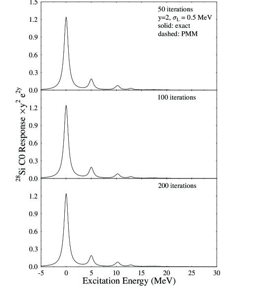
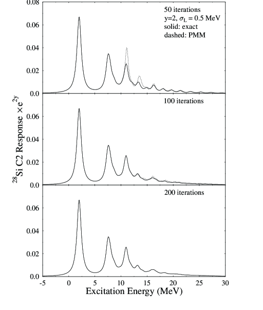
Figure 1: Comparison of an exact moments calculation (solid line) with the PMM (dashed) method for the C0 and C2 response functions along the $y$=2 line in the response plane.

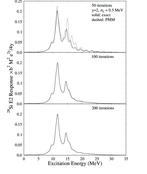
Figure 2: As in Fig. 1, only for the E2 response.

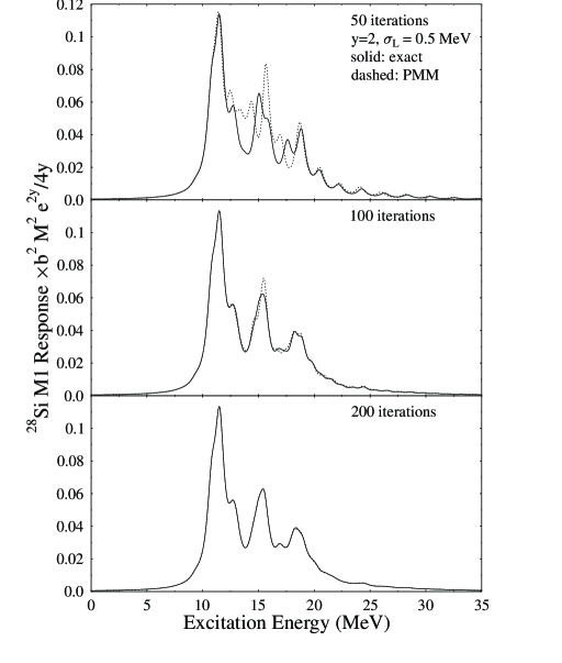
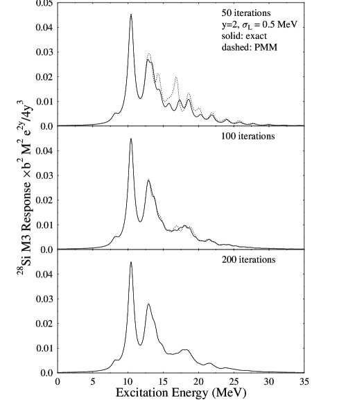
Figure 3: As in Fig. 1, only for the m1 and M3 responses.

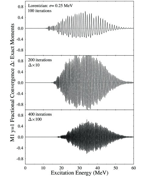
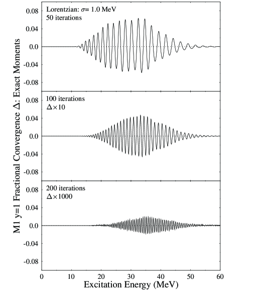
Figure 4: Comparison of the convergence of the M1 response for $y$=1 for $\sigma$ = 0.25 and 1.0 MeV in an exact moments calculation.

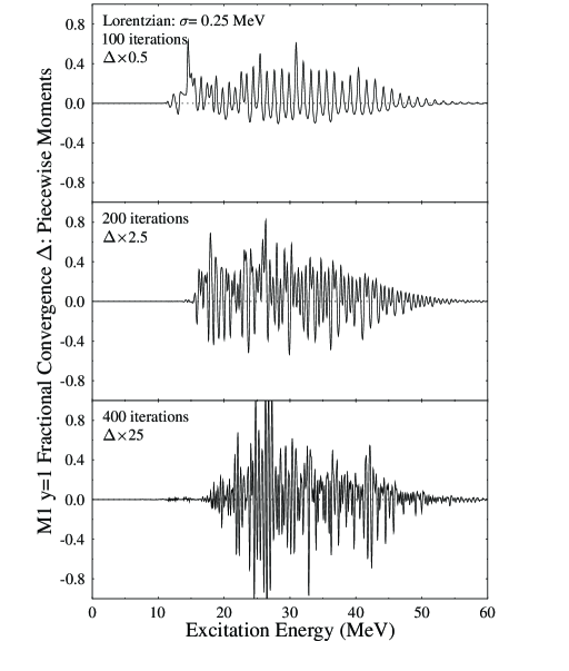
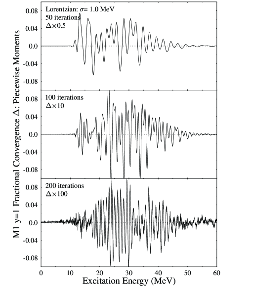
Figure 5: As in Fig. 4, only for the PMM calculation.

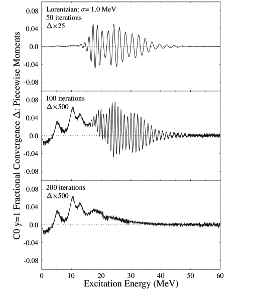
Figure 6: Convergence of the PMM C0 response for $y$=1 and $\sigma$=1.0 MeV. A small difference persists near the dominant extremum eigenvalues.

All of these response functions were evaluated with the PMM, for several resolution-function widths ($\sigma$=1.0, 0.5, and 0.25 MeV) and for $n$ ranging from 50 to 400 iterations. The results we show all assume a Lorentzian for the resolution function. The accuracy of the PMM was first tested by examining cuts corresponding to $y$=constant in the $(\omega,q)$ plane. For such trajectories, $O(y)$ is fixed, so that Eq. 5 can be used – an exact moments treatment. This will allow us to test our qualitative argument that the PMM should be numerically difficult to distinguish from an exact moments treatment, provided $n$ is large enough for the given $\sigma$. Figures 1-3 show the results for the C0, C2, E2, M1, and M3 response functions – the cases with more than one component in the vector $|v_{1}(y)\rangle$ – for $y$=2 and $\sigma$=0.5 MeV, and with $n$=50,100, and 200.

In those cases where there is significant structure in the response function, discrepancies are apparent at $n$=50, but these disappear as more iterations are added. In all cases, by $n$=200 differences between an exact moments calculation and the PMM result are not readily discernible on the scale of the graphs. Note that the differences at $n$=50 reflect that fact that neither the exact moments calculations nor the PMM results are fully converged. Similar results were obtained for $y$=1. This kind of test could be made by anyone using the PMM, to guarantee, for the chosen resolution function and $\sigma$, that a sufficient number of iterations have been done to produce the desired accuracy.

The next series of figures provide a more detailed look at the convergence and its dependence on $\sigma$. Fig. 4 provides benchmarks for exact moments calculations, the residual discrepancies between calculations for $n$=50, 100, 200, and 400 iterations and one with $n$=600, which we will take as a fully converged result. The figures show the convergence in the case of the M1 response evaluated along the line $y$=1 at the resolutions $\sigma$ = 0.25 and 1.0 MeV. The behavior is just as one would expect. The missing contributions are oscillatory, with a frequency that is roughly proportional to $n$ but virtually independent of $\sigma$, for the range we explored. The envelope of the oscillations decreases with increasing $n$, shrinking by more than an order of magnitude for every additional 50 iterations for $\sigma$=1.0 MeV. The decrease slows to about a factor of 5 every 100 iterations for the more taxing calculation with $\sigma$=0.25 MeV.

Similar calculations, not shown, were performed for the C0 response, which has much less structure than the M1 response. The results are qualitatively similar to that shown in Fig. 4, though the convergence of the envelope is a factor of $\sim$ 30 more rapid.

Figure 5, the analog of Fig. 4, gives the M1 PMM residuals (again relative to an exact moments calculation with $n$=600). While again an oscillatory pattern emerges with a frequency like that of Fig. 4, its structure is less regular. This is the result of the interference between the three Lanczos patterns that contribute to the PMM result, corresponding to the starting vectors $|v_{1}^{0}\rangle$, $|v_{1}^{1}\rangle$, and $|v_{1}^{2}\rangle$. The PMM envelopes tend to be a factor of two to three more extended than those from the exact moments calculation, though in one case the difference is larger.

Figure 6, the residuals for the PMM calculation for the C0 response, with $y$=1 and $\sigma$ = 1.0 MeV, show an interesting effect. Through most of the spectrum the same oscillatory features and diminishing envelope with increasing $n$ are seen. But in the low-energy region, a persistent feature has converged by $n$=100. It appears dominantly positive, but as the fractional convergence is graphed and as this response is dominated by the ground state, where the differential is negative, this is misleading. The low-energy C0 response is characterized by isolated extremum eigenvalues, as is apparent from Fig. 1, with the ground state carrying the entire response from $|v_{1}^{0}\rangle$ ($y\rightarrow$ 0). These appear to be conditions that allow for a small deviation of the PMM from the results of an exact moments calculation, in converged calculations. However, the deviation is small, less than 0.01%. Very similar effects were found in the C0 responses for $\sigma$ = 0.5 MeV and 0.25 MeV, with the discrepancies reaching 0.03% and 0.06% in these cases, respectively.

Finally, we show a series of PMM results for the response surface. Figure 7 shows contour plots for the C0, C2, and C4 responses, while Figs. 8 and 9 give the three-dimensional projections of the E2 and E4 and the M1, M3, and M5 responses, respectively. The general shift of strength to larger $y$ with increasing multipolarity is apparent. In most applications of the PMM, such response surfaces, determined as a function not only of $(\omega,q)$ but also of the oscillation parameter $b$, would be the end result of the calculations.

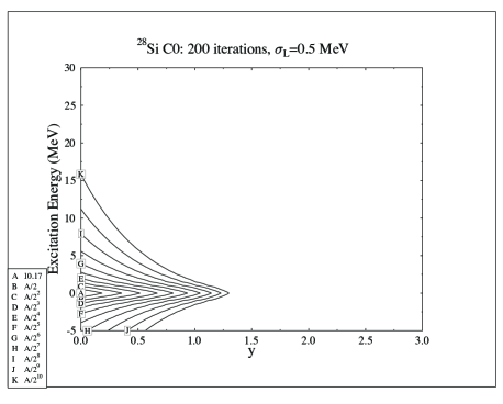
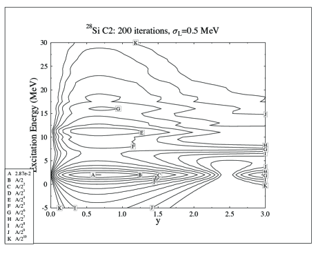
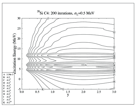
Figure 7: The PMM response surfaces for the C0, C2, and C4 multipoles, with contours drawn at successive factors of 0.5 of the maximum, until 0.001 is reached.

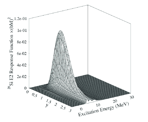
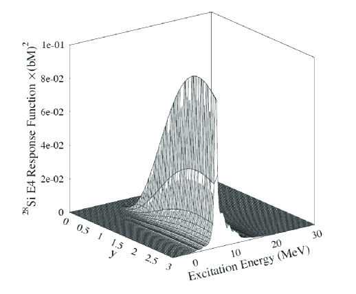
Figure 8: The PMM response surface for the E2 and E4 multipoles.

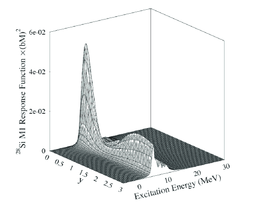
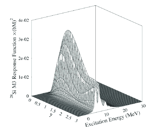
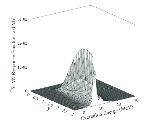
Figure 9: As in Fig. 8, only for the M1, M3, and M5 responses.

VI Conclusions

An attractive property of the matrix elements of electroweak single-particle operators between harmonic oscillator states is that they can be evaluated analytically, yielding a simple form that includes a finite polynomial in $y=(qb/2)^{2}$. This property has been exploited frequently in calculations of discrete transition amplitudes. In this paper we have shown that moments methods exploiting this property can very efficiently characterize the entire response surface over the $(\omega,q)$ plane. This can be viewed as an important extension of well-known moments techniques for determining the distribution of Gamow-Teller strength along the line $q=0$ in the $(\omega,q)$ plane.

While the method was motivated by the observation that moments must have a polynomial form in $y$, algorithms we designed to exactly preserve the moments were found to be numerically unstable, if a sufficient number of iterations $n$ were done. This difficulty is the well-known “classical moments problem,” the determination of a discrete distribution from knowledge of the distribution’s moments. An alternative method, called the Piecewise Moments Method, was introduced in which each polynomial component of the starting vector was treated separately in the Lanczos procedure, while also incorporating a resolution function directly into the algorithm. The method is extremely stable, positive definite, and effectively equivalent, numerically, to an exact moments reconstruction. After convergence – which typically requires $\sim$ 200 iterations for a resolution $\sigma\sim$ 0.5 MeV – we found maximal differences between the PMM and exact moments calculations of about 0.01%, in one case (the C0 multipole). The number of iterations $n$ required for convergence increases with decreasing $\sigma$.

We noted that the absence of a moments method to reconstruct the response in the full $(q,\omega)$ plane had previously led to the use of very simple nuclear models, so that state-by-state sums over transitions could be performed. Clearly the PMM will now allow theorists to perform analogous calculations using state-of-the-art shell-model wave functions in very large model spaces. The efficiency with which the PMM constructs the response function over the response plane is impressive. In the example we explored – the electromagnetic form factors for ²⁸Si in the $sd$-shell – the most complicated multipoles, C0 and M1, required only three Lanczos steps.

Another aspect of the method, discussed in Section II, is that it can be viewed as a numerical effective theory in the sense that exactly that information needed to reconstruct $S(\omega,q)$ can be systematically extracted from exceedingly complicated nuclear structure calculations. Specifically, if $n$ is the number of iterations and $m$ the rank of $p(y)$, one needs $(m+1)(2n-1)$ tridiagonal Lanczos matrix elements and $[m(m-1)/2]n^{2}$ Lanczos vector overlaps to implement Eq. IV, for example. Once this information is in hand, a simple routine could be coded to generate $S(\omega,q)$ as a continuous function of $\omega$ and $q$, as well as of the oscillator parameter $b$ and $\sigma$. (The one caveat in that for any fixed $n$, there will be some minimum $\sigma$ beyond which the number of iterations $n$ performed would not be sufficient.) In effect, $S(\omega,q)$ would be no more complex, in numerical calculations, than some analytically known leptonic scattering kernel. One application we have in mind is neutrino reactions in core-collapse supernova modeling. This approach would allow one to model such reactions with state-of-the-art shell model techniques, yet produce a result sufficiently simple that it could be used on-line within a sophisticated supernova code. The fact that $S(\omega,q)$ is given as a function of $\omega$ and $q$, rather than as a grid of values, is also important in such applications. This will allow supernova modelers to more easily guarantee properties such as detailed balance in reactions and inverse reactions – which if not enforced exactly, can lead to energy generation and other spurious physics when weak interactions are in equilibrium. Detailed balance can be more difficult to enforce in cases where $S(\omega,q)$ is provided on some discrete numerical grid.

We would like to mention three follow-up studies that we think will make the present work more valuable. First is the extension to weak interactions. This is relatively simple, as only two new operators (in addition to those we have treated in Eqs. 31 and 43) arise when axial currents are added (in the standard nonrelativistic treatment where charges and currents are kept to order $1/M$) walecka ; donnelly . One of the main motivations of the present paper is to develop a technique that can be applied to neutrino response functions in the energy range up to $\sim$ 1 GeV.

A second question is the loss of unitarity for momentum-dependent operators acting in finite shell model spaces. This issue does not arise for the standard application to the Gamow-Teller operator $g_{A}^{eff}\sigma\tau_{\pm}$, for any complete $n\hbar\omega$ shell-model space, as the operator has no cross-shell matrix elements. But for more general operators, as the momentum increases, so does the strength of excitations to states outside the model space. For a vector $O(y)|g.s.\rangle$ it is simple exercise to calculate the loss of probability due to excitations outside the model space. If one fails to take into account such loss of probability, trends in inclusive cross sections as a function of $q$ will be distorted. Thus it is important to either correct for such effects, or to evaluate their size to estimate uncertainties in results.

A third issue is the overcompleteness of shell-model spaces due to spurious center-of-mass motion. This can be troublesome when dealing with one-body operators that can excite center-of-mass excitations. While this issue did not arise in our example of ²⁸Si because we confined ourselves to the 0 $\hbar\omega$ $sd$-shell space, it will in more complicated spaces. If the space is separable – e.g., any $n\hbar\omega$ shell-model calculation with oscillator wave functions – the standard technique, when dealing with discrete calculations, is to remove spurious states by adding to the Hamiltonian a term $\alpha H_{CM}$, where $H_{CM}$ is the center of mass Hamiltonian and $\alpha\sim$ 100 a coefficient chosen to “blow out” spurious states from the low-energy spectrum whit2 . This works well for converged Lanczos calculations: the addition of such a term forces low-lying eigenvalues to have the center-of-mass in the $1s$ state. One would need to explore numerically whether a similar technique might allow some approximate separation of spurious excitations over the full spectrum: we are not aware of any studies of this method apart from the case of converged extremal eigenvalues. Alternatively, if the shell-model Hamiltonian is (properly) translationally invariant and $|g.s.\rangle$ has been constructed so that its center of mass is in the $1s$ state, center-of-mass excitations in the vector $O(y)|g.s.\rangle$ could be removed at the outset.

Appendix A Alternative Methods

In this Appendix we discuss in more detail alternative Lanczos response function methods that we have explored. This discussion might be useful to those that would like to further explore some of the stability issues we encountered. The first two approaches have as their goal a reconstruction of $S(\omega,q)$ that exactly captures the information in the $2n-1$ moments. The main drawback in both methods is instability for moderate $n$, connected with the classical moments problem (the inversion from moments to a distribution). A third method is discussed which deals directly with distributions while also preserving a specified number of moments.

A.1 Naive Moments Method

As discussed in the main body of the paper, the NMM begins with a starting vector of the form

$$c(y)|v_{1}(y)\rangle=c_{0}|v_{1}^{0}\rangle+c_{1}y|v_{1}^{1}\rangle+\dots+c_{m}y^{m}|v_{1}^{m}\rangle$$ (48)

from which the moments $\langle v_{1}(y)|H^{\lambda}|v_{1}(y)\rangle$, $\lambda=1,\dots,2n-1$, can be determined for any $y$ once the mixed moments $\Omega_{ij}^{\lambda}$ have been evaluated. As knowledge of the moments as a function of $y$ is mathematically equivalent to knowledge of $L(n,|v_{1}(y)\rangle)$, the response function can thus be evaluated as a function of both $y$ and $\omega$.

On first sight, it appears that the inversion from moments to the tridiagonal matrix can be easily done. It has been shown akhiezer that the elements of the Lanczos matrix are related to the moments by determinants so that

$$\alpha_{i}=\mathcal{M}_{i-1}/\mathcal{L}_{i-1}-\mathcal{M}_{i-2}/\mathcal{L}_{i-2}$$ (49)

and

$$\beta_{i}=\mathcal{L}_{i}^{1/2}\mathcal{L}_{i-2}^{1/2}/\mathcal{L}_{i-1},$$ (50)

where the determinants $\mathcal{L}$ and $\mathcal{M}$ are defined by

$$\mathcal{L}_{n}=\left|\begin{array}[]{ccccc}1&\mu_{1}&\mu_{2}&\cdots&\mu_{n}\\ \mu_{1}&\mu_{2}&\mu_{3}&\cdots&\mu_{n+1}\\ &\vdots&&&\vdots\\ \mu_{n}&\cdots&&&\mu_{2n}\\ \end{array}\right|$$ (51)

and

$$\mathcal{M}_{n}=\left|\begin{array}[]{cccccc}1&\mu_{1}&\mu_{2}&\cdots&\mu_{n-1}&\mu_{n+1}\\ \mu_{1}&\mu_{2}&\mu_{3}&\cdots&\mu_{n}&\mu_{n+2}\\ &\vdots&&&\vdots&\vdots\\ \mu_{n}&\cdots&&&\mu_{2n-1}&\mu_{2n+1}\\ \end{array}\right|,$$ (52)

with $\mu_{\lambda}\equiv\langle v_{1}|H^{\lambda}|v_{1}\rangle$, and with $\mathcal{M}_{-1}$=0, $\mathcal{M}_{0}=\mu_{1}$, and $\mathcal{L}_{0}$=1. The NMM uses these equations to determine the Lanczos matrix $L(n,|v_{1}(y)\rangle$ from the $\mu_{\lambda}(y)$. Then one can proceed in the usual way to diagonalize this matrix and then construct the strength function, using Eq. 7.

While sound mathematically, the NMM is problematic numerically because the solution to the classical moments problem embodied in Eqs. 49 and  50 is not a stable one. For example, Whitehead and Watt provide in Ref. whit3 a simple 4 $\times$ 4 matrix example in which significant loss of accuracy occurs.There have been attempts fletcher91 ; nair82 to finite alternate methods that use moments in a manner that will improve the inversion to a distribution. None of these have proven to have the stability of a direct Lanczos construction, however. In the numerical tests we performed, significant errors typically occurred for $n\sim 20$, in calculations performed with 64-bit accuracy. As is apparent from many of the calculations presented in this paper, often 50-200 iterations are required before a response function is accurately reconstructed, for resolutions we explored.

A.2 Legendre Moments Method

Operationally, the rapid loss of precision in the NMM occurs because of severe cancellations in the determinants (Eqs. 51 and 52) that arise from the dominance of the largest eigenvalues in the highest-order moments. This dominance occurs because naive moments methods work with a set of non-orthogonal basis vectors: $H^{n}|v_{1}\rangle$ with $n$ non-negative integers. The Lanczos algorithm, on the other hand, builds a set of orthogonal vectors $|v_{n}\rangle$ as it goes, each carrying information about $H$ that is independent from that in its predecessors, and this produces the great stability of the algorithm.

We attempted to find a new way to iterate for $\alpha_{i}$ and $\beta_{i}$ in terms of moments that, like the original Lanczos algorithm, are built on a set of orthogonal vectors, $|w_{i}\rangle$, constructed as part of the iteration. We describe a first attempt at an iterative method, which fails because it is equivalent to the NMM. We then give a closely analogous procedure based on linear combinations of moments that proved, at times, to be considerably more stable.

We begin as in the NMM procedure by calculating the mixed moments $\Omega^{\lambda}_{ij}$, from which we can then evaluate the moments $\langle v_{1}(y)|H^{m}|v_{1}(y)\rangle$ as a function of $y$.

We then build up the orthogonal vectors $|w_{i}\rangle$ of dimension $i$ iteratively, starting with

$$|w_{1}\rangle=\left(\alpha_{1}\right)$$ (53)

$$|w_{2}\rangle=\left(\begin{array}[]{c}\alpha_{1}\\ \beta_{1}\end{array}\right),$$ (54)

where $\alpha_{1}$, $\beta_{1}$ are easily identified from the moments $\langle v_{1}|H|v_{1}\rangle=\alpha_{1}$ and $\langle v_{1}|H^{2}|v_{2}\rangle-\alpha_{1}^{2}=\beta_{1}^{2}$ (defined as in ordinary Lanczos). With these vectors in hand we compute the next $\alpha_{i}$, $\beta_{i}$, and $|w_{n}\rangle$ from

$$\alpha_{n}=\frac{\langle v_{1}|H^{2n-1}|v_{1}\rangle-\langle w_{n-1}|L_{n-1}|w_{n-1}\rangle}{\beta_{1}^{2}\beta_{2}^{2}\cdots\beta_{n-1}^{2}}$$

$$-2(\alpha_{1}+\alpha_{2}\cdots+\alpha_{n})$$ (55)

$$\beta_{n-1}^{2}=\frac{\langle v_{1}|H^{2n-2}|v_{1}\rangle-\langle w_{n-1}|w_{n-1}\rangle}{\beta_{1}^{2}\beta_{2}^{2}\cdots\beta_{n-2}^{2}}$$ (56)

$$|w_{n}\rangle=L_{n}\left(\begin{array}[]{c}|w_{n-1}\rangle\\ \beta_{1}\beta_{2}\cdots\beta_{n-1}\end{array}\right),$$ (57)

where $L_{n}$ is the truncated Lanczos matrix of Eq. 2.

In this way we construct the Lanczos matrix, which can then be diagonalized and used to derive the response function in the usual way. This algorithm yields significant stability improvements over the procedure outlined in the NMM discussion. However, the new algorithm still suffers from cancellations between terms in both Eqs. 55 and 56. Successively higher moments yield increasingly large numbers on each side of the minus signs in those equations. These numbers are subtracted to yield successive $\alpha_{i}$ and $\beta_{i}$ that remain of order unity. Such large cancellations lead to loss of precision that, though less severe than in naive moments methods, has the same root and the same consequence of failure in that eventually $\beta_{n}^{2}<0$. At this point the algorithm fails.

One possible solution to this problem is to find combinations of moments that remain relatively stable in size, e.g., some set of orthogonal polynomials. If we scale and shift energies so that the range of eigenvalues can be mapped onto [-1,1], one obvious choice would be Legendre polynomials. They contain the same information as the moments, and their matrix elements will have the same dependence in $y$. However, as they have a fixed magnitude at the endpoints, they are not overwhelmed by the extremal eigenvalues for large $n$. In the LMM the moments of the NMM are replaced by

$$\langle v_{1}|\hat{P}_{0}^{2}|v_{1}\rangle \equiv \langle q_{0}|q_{0}\rangle$$

$$\langle v_{1}|\hat{P}_{1}^{2}|v_{1}\rangle \equiv \langle q_{1}|q_{1}\rangle$$

$$\langle v_{1}|\hat{P}_{1}H\hat{P}_{1}|v_{1}\rangle = \langle q_{1}|H|q_{1}\rangle$$

$$\langle v_{1}|\hat{P}_{2}^{2}|v_{1}\rangle \equiv \langle q_{2}|q_{2}\rangle$$

$$\langle v_{1}|\hat{P}_{2}H\hat{P}_{2}|v_{1}\rangle = \langle q_{2}|H|q_{2}\rangle$$

$$\vdots$$

The operators $\hat{P}_{l}(H)$ are linear combinations of powers of $H$, with coefficients identical to those on the corresponding powers of the scalar $x$ in the Legendre polynomials $P_{l}(x)$. Instead of computing moments, we calculate the overlaps $\langle q_{l}|q_{l}\rangle$, using the Legendre polynomial recurrence relation to generate $|q_{l}\rangle$. The vectors $|q_{l}\rangle$ have a simple expansion in $y$ because they are built from linear combinations of the $|v_{1}^{i}\rangle$, so

$$|q_{l}\rangle=|q_{l}^{1}\rangle+|q_{l}^{2}\rangle y+\cdots|q_{l}^{n}\rangle y^{n-1},$$ (58)

and $|q_{l}^{i}\rangle$ is easily computed from $|v_{1}^{i}\rangle$ at the start of the calculation. The recurrence relations used are then

$$|q_{0}^{i}\rangle = |v_{1}^{i}\rangle$$ (59)

$$|q_{1}^{i}\rangle = H|v_{1}^{i}\rangle$$ (60)

$$|q_{l+1}^{i}\rangle = \frac{2l+1}{l+1}H|q_{l}^{i}\rangle-\frac{l}{l+1}|q_{l-1}^{i}\rangle.$$ (61)

It is straighforward to find the Lanczos matrix $L_{n}$ in terms of the $\langle q_{n}|q_{n}\rangle$. This resulting inversion – from Legendre moments to the tridiagonal matrix – proved to be significantly more stable than the NMM inversion. The recurrence relations to compute $L_{n}$ are

$$\alpha_{n}=\frac{\langle q_{n-1}|H|q_{n-1}\rangle-\langle w_{n-1}|L_{n-1}|w_{n-1}\rangle}{\beta_{1}^{2}\beta_{2}^{2}\cdots\beta_{n-1}^{2}}$$

$$-2\left(\frac{(2n-3)!!}{(n-1)!}\right)^{2}(\alpha_{1}+\alpha_{2}\cdots+\alpha_{n})$$ (62)

$$\beta_{n-1}^{2}=\left(\frac{(n-1)!}{(2n-3)!!}\right)^{2}\frac{\langle q_{n-1}|q_{n-1}\rangle-\langle w_{n-1}|w_{n-1}\rangle}{\beta_{1}^{2}\beta_{2}^{2}\cdots\beta_{n-2}^{2}},$$ (63)

$$|w_{n}\rangle=\left(\frac{2n-3}{n-1}\right)L_{n}\left(\begin{array}[]{c}|w_{n-1}\rangle\\ 0\end{array}\right)$$ (66)

$$-\left(\frac{n-2}{n-1}\right)\left(\begin{array}[]{c}|w_{n-2}\rangle\\ 0\\ 0\end{array}\right)$$ (70)

with $|w_{1}\rangle$, $|w_{2}\rangle$, $\alpha_{1}$, and $\beta_{1}$ as before.

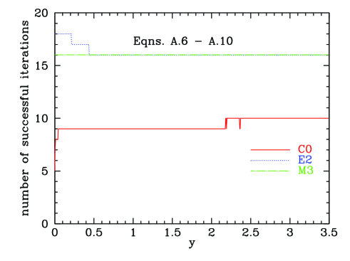
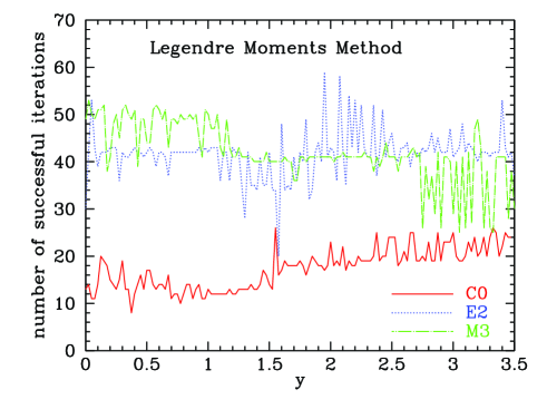
Figure 10: The number of iterations before loss of precision produces $\beta_{i}<0$ in the moments algorithms, for each operator computed in our ²⁸Si example case, as functions of momentum transfer. The upper graph is the result for the method of Eqs. 53–57 , while the bottom graph gives the Legendre Moments Method (Eqs. 62–70).

These two moments methods (Eqs. 55–57 and Eqs. 62–70) are defined by similar procedures. We compare their stability in Fig. 10. In our experience, the Legendre moments algorithm can sometimes run to very high numbers ($>80$) of iterations with no significant loss of precision, but it also sometimes runs aground quickly on cancellations in Eq. 63. The lack of predictability is clearly an issue.

Our failure to identify a more reliable method for determining distributions from moments motivated us to look for other approaches, e.g., ones that might not capture exact information on the moments at every $y$ or exactly guarantee positive-definiteness of the response function, but would remain stable and accurate under continued iteration. This led to the PMM method we favor, as well as one other moment-preserving approach described below.

A.3 Legendre Coefficients Method

Rather than constructing a Lanczos matrix, diagonalizing, and finding the strength distribution, an approximate strength distribution can be computed directly from an expansion in Legendre polynomials,

$$S(\omega,y)=y^{J-K}e^{-2y}\sum_{l=0}^{\infty}a_{l}(y)P_{l}(\omega).$$ (71)

The coefficients $a_{l}(y)$ can be computed using the orthogonality relation for Legendre polynomials and the identity

$$y^{J-K}e^{-2y}|c(y)|^{2}\langle v_{1}|\hat{P}_{l}(H)|v_{1}\rangle=\int S(\omega,y)P_{l}(\omega)d\omega,$$ (72)

so that

$$a_{l}(y)=\frac{2l+1}{2}|c(y)|^{2}\langle v_{1}|\hat{P}_{l}(H)|v_{1}\rangle.$$ (73)

We refer to the method of computing response functions from Legendre coefficients computed with these relations as the “Legendre coefficients” method.

Here again, $H$ must be shifted and scaled to the interval $\left[-1,1\right]$ before calculating these matrix elements, then shifted and scaled back at the end to obtain the true strength distribution. A numerically stable approach to calculating the $a_{l}(y)$ uses the same vectors $|q_{n}\rangle$ defined for the Legendre moments method, constructed in the same way, so that

$$a_{l}(y)=\frac{2l+1}{2}\sum_{j,k=0}^{m}c_{j}c_{k}y^{j+k}\langle v_{1}^{k}|q_{l}^{j}\rangle,$$ (74)

where $c_{j}$ are defined in Eq. 48.

The approximate strength function $S_{LC}^{n}$ represented by the first $n$ Legendre polynomials will always contain oscillations about the true strength function, at an energy scale given by the order of the highest Legendre polynomial in the expansion, so roughly on the scale $\Delta\omega/n$, where $\Delta\omega$ is the difference between the maximum and minimum eigenvalues of $H$. (Since the true response function is a sum of delta functions, its expansion in Legendre polynomials never truncates.) There is no restriction on the sign of $S_{LC}^{n}(\omega,y)$, so its oscillations may make it negative in places even though $S(\omega,y)$ is strictly positive. For these reasons, practical use of this method would probably require smoothing smoothing the function $S_{LC}^{n}(\omega,y)$ to finite resolution over scales of approximately $\Delta\omega/n$. Since we have a Legendre expansion of $S_{LC}^{n}$, the convolution to produce the smoothed function may be performed efficiently (i.e., reduced to a series of matrix multiplications) by working with Legendre expansions of the smoothing function. The Legendre coefficient expansion may be useful in applications where the response function needs to be convolved with some other function, for example, a thermal energy distribution. On the other hand, while the Lanczos methods converge more rapidly at the ends of the eigenvalue spectrum than in the middle, that is not in general the case for the Legendre expansion.

We also note that, whereas the ordinary Lanczos algorithm and our variants on it need to run $n$ iterations on each vector piece to reproduce $2n-1$ moments of the response function, the Legendre coefficients methods needs to run $2n-1$ iterations to produce $2n-1$ moments, essentially twice as long as the other methods in this Appendix. As in the Lanczos method, each iteration contains as its basic time-consuming step a matrix-vector multiplication in the original large basis.

It has come to our attention that a closely-related method is in use in physical chemistry, where it is used to compute the quantum-mechanical time evolution of molecular states wall95 ; kosloff87 . Authors working in that area point out that if Chebyshev polynomials are used instead of Legendre polynomials, the vectors $|q_{l}\rangle$ may still be found by recurrence, but only the first $n$ such vectors need to be computed in order to find the first $2n$ terms of the expansion in Chebyshev polynomials.

References

- (1) E. Caurier, G. Martinez-Pinedo, F. Nowacki, A. Poves, and A. P. Zuker, nucl-th/0402046/ (Rev. Mod. Phys., in press)
- (2) B. A. Brown and B. H. Wildenthal, Ann. Rev. Nucl. Part. Sci. 38, 29 (1988); S. Cohen and D. Kurath, Nucl. Phys. 73, 1 (1965.
- (3) W. C. Haxton and C. L. Song, Phys. Rev. Lett. 84, 5484 (2000); P. Navratil, J. P. Vary, and B. R. Barrett, Phys. Rev. Lett. 84, 5728 (2000); S. Bogner, T. T. S. Kuo, L. Coraggio, A. Covello, and N. Itaco, Phys. Rev. C65, 051301 (2002); T. S. Luu, S. Bogner, W. C. Haxton, and P. Navratil, Phys. Rev. C.70, 014316 (2004).
- (4) C. Lanczos, J. Res. Nat. Bur. Stand. 45, 255 (1950); J. H. Wilkinson, The Algebraic Eigenvalue Problem (Clarendon Press, Oxford, 1965).
- (5) K. Langanke and G. Martinez-Pinedo, Nucl. Phys. A673, 481 (2000); E. Caurier, K, Langanke, G. Martinez-Pinedo, and F. Nowacki, Nucl. Phys. A653, 439, 1999.
- (6) A. Heger, S. E. Woosley, G. Martinez-Pinedo, and K. Langanke, Astrophys. J. 560, 307 (2001).
- (7) W. R. Hix, O. E. B. Messer, A. Mezzacappa, M. Liebendoerfer, J. Sampaio, K. Langanke, D. J. Dean, and G. Martinez-Pinedo, Phys. Rev. Lett. 91, 201102 (2003).
- (8) W. C. Haxton, Phys. Rev. Lett. 60, 1999 (1988); S. E. Woosley, D. H. Hartmann, R. D. Hoffman, and W. C. Haxton, Astrophys. J. 356, 272 (1990).
- (9) J. Cullum and R. Willoughby, Lanczos Algorithms for Large Symmetric Eigenvalue Computations, vol, 1 (Birkhäuser, Boston, 1985)
- (10) R. R. Whitehead, in Moment Methods in Many Fermion Systems, ed. B. J. Dalton, S. M. Grimes, J. P. Vary, and S. A. Williams (Plenum Press, New York, 1980), p. 235.
- (11) R. R. Whitehead et al., Adv. in Nucl. Phys. 9, 123 (1977).
- (12) R. Haydock, J. Phys. A7, 2120 (1974); R. Haydock, in Computational Methods in Classical and Quantum Physics, ed. M. B. Hooper (Advance Publications, London, 1976), p. 268.
- (13) J. Engel, W. C. Haxton, and P. Vogel, Phys. Rev. C46, 2153 (1992).
- (14) T. DeForest, Jr., and J. D. Walecka, Adv. Phys. 15, 1 (1966); J. D. Walecka, in Muon Physics, ed. V. W. Hughes and C. S. Wu (Academic Press, New York, 1975), p. 113.
- (15) T. W. Donnelly and W. C. Haxton, Atomic Data and Nucl. Data Tables 23, 103 (1979).
- (16) There have been applications of Lorentz transform methods to few-body nuclei, including one that employed Lanczos techniques, though the approach and motivations differ from those under discussion here. See, for example, M. A. Marchisio, N. Barnea, W. Leidemann, and G. Orlandini, Few-Body Syst. 33, 259 (2003) and nucl-th/0202009/.
- (17) N. Akhiezer, The Classical Moment Problem (Oliver and Boyd, Edinburgh,1965).
- (18) R. R. Whitehead and A. Watt, J. Phys. G 4, 835 (1978) and J. Phys. A 14, 1887 (1981).
- (19) J. Fletcher, J. Phys. A 24, L7 (1991).
- (20) C. Radhakrishnan and S. Nair, Phys. Lett. 91A, 64 (1982).
- (21) M. R. Wall and D. Neuhauser, J. Chem. Phys. 102, 8011 (1995).
- (22) R. Kosloff, J. Phys. Chem. 92, 2087 (1987).