Relativistic Continuum Hartree Bogoliubov Theory for Ground State Properties of Exotic Nuclei

Abstract

The Relativistic Continuum Hartree-Bogoliubov (RCHB) theory, which properly takes into account the pairing correlation and the coupling to (discretized) continuum via Bogoliubov transformation in a microscopic and self-consistent way, has been reviewed together with its new interpretation of the halo phenomena observed in light nuclei as the scattering of particle pairs into the continuum, the prediction of the exotic phenomena — giant halos in nuclei near neutron drip line, the reproduction of interaction cross sections and charge-changing cross sections in light exotic nuclei in combination with the Glauber theory, better restoration of pseudospin symmetry in exotic nuclei, predictions of exotic phenomena in hyper nuclei, and new magic numbers in superheavy nuclei, etc. Recent investigations on new effective interactions, the density dependence of the interaction strengthes, the RMF theory on the Woods-Saxon basis, the single particle resonant states, and the resonant BCS (rBCS) method for the pairing correlation, etc. are also presented in some details.

Key words

Relativistic mean field theory, continuum, pairing correlation, Bogoliubov transformation, relativistic continuum Hartree-Bogoliubov, exotic nuclei, halo, giant halo, hyperon halo, interaction cross section, charge-changing cross section, pseudospin symmetry, hyper nuclei, magic number, superheavy nuclei.

1 Introduction

Currently nuclear physics is undergoing a renaissance as evidenced by the fact that worldwide there are lots of Radioactive Ion Beam (RIB) [1] facilities operating, being upgraded, under construction or planning to be constructed, e.g., the Cooling Storage Ring (CSR) project at HIRFL in China will be completed in 2005 [2], the RIB Factory at RIKEN in Japan will begin to operate at the end of 2006 [3], the FAIR project at GSI in Germany was approved in 2003 [4], and the construction of the Rare Isotope Accelerator (RIA) is considered to be of the highest priority of all physics disciplines in the US [5], etc. These new facilities together with developments in the detection techniques have changed the nuclear physics scenario. It has come into reality to produce and study the nuclei far away from the stability line — so called “EXOTIC NUCLEI” [6, 7, 8, 9, 10, 11, 12].

New exciting discoveries have been made by exploring hitherto inaccessible regions in the nuclear chart [6, 7, 8, 9, 10, 11, 12]. For examples, a new phenomenon, halo — a state in which nucleons spread like a thin mist around the nucleus, was first discovered in ¹¹Li with RIB in 1985 [13] and later in many other light exotic nuclei as well; exotic nuclei exhibit other interesting phenomena such as the disappearance of traditional shell gaps and the occurrence of new ones, which result in new magic numbers [14]; etc. The exotic nuclei also play important roles in nuclear astrophysics as well, as their properties are crucial to understand stellar nucleosynthesis.

The current nuclear models are mainly based on the knowledge obtained from the nuclei near the $\beta$-stability line. For instances, the cornerstones for the edifice of modern nuclear physics include shell model [15] and collective model [16, 17], which are respectively based on the magic numbers (the stability of some nuclei compared with their neighbors) and the incompressibility of the nuclear matter. Therefore the change of magic numbers and the unprecedented low density nuclear matter in halo nuclei have shaken the foundation of nuclear physics. New innovative nuclear models are needed to describe the exotic nuclei characterized by weakly binding and low density.

The relativistic mean field (RMF) theory [18] has received wide attention due to its successful description of lots of nuclear phenomena during the past years [19, 20, 21, 22, 23]. In the framework of the RMF theory, the nucleons interact via the exchanges of mesons and photons. The representations with large scalar and vector fields in nuclei, of order of a few hundred MeV, provide simpler and more efficient descriptions than nonrelativistic approaches that hide these scales. The dominant evidence is the spin-orbit splittings. Other evidence includes the density dependence of optical potential, the observation of approximate pseudospin symmetry, correlated two-pion exchange strength, QCD sum rules, and more [24]. The relativistic Bruekner-Hartree-Fock theory and RMF theory with density-dependent coupling constants extracted from it can reproduce well the nuclear saturation properties (the Coester line) in nuclear matter [25, 26]. Furthermore the RMF theory can reproduce better the measurements of the isotopic shifts in the Pb-region [27], give more naturally the spin-orbit potential, the origin of the pseudospin symmetry [28, 29] as a relativistic symmetry [30, 31, 32] and spin symmetry in the anti-nucleon spectrum [33], and be more reliable for nuclei far away from the line of $\beta$-stability, etc. Obviously, RMF is one of the best candidates for the description of exotic nuclei.

In order to describe exotic nuclei, the pairing correlation and the coupling to continuum, which are extremely crucial for the description of drip line nuclei, must be taken into account properly [34]. The continuum effect is commonly taken into account in the Hartree-Fock-Bogoliubov (HFB) [35] or relativistic-Hartree-Bogoliubov (RHB) [21] approaches. In most of these calculations the continuum is replaced by a set of positive energy states determined by solving the HFB or RHB equations in coordinate space and with box boundary conditions [36, 37, 38]. Recently the HFB equations were also solved with exact boundary conditions for the continuum spectrum, both for a zero range [39] and a finite range pairing forces [40]. These resonant continuum HFB or RHB results with exact boundary conditions are generally close to those with box boundary conditions [39, 41]. The extension of the RMF theory to take into account both bound states and (discretized) continuum via Bogoliubov transformation in a microscopic and self-consistent way, i.e., the Relativistic Continuum Hartree-Bogoliubov (RCHB) theory has been done in Refs. [36, 42]. The RCHB theory was very successful in describing the ground state properties of nuclei both near and far from the $\beta$-stability line. By using a density-dependent zero range interaction, the halo in ¹¹Li has been successfully reproduced in this self-consistent picture. Remarkable successes of the RCHB theory include the new interpretation of the halo in ¹¹Li [36], the prediction of the exotic phenomena as giant halos in Zr ($A>122$) [43] and Ca ($A>60$) [44] isotopes, the reproduction of interaction cross section and charge-changing cross sections in light exotic nuclei in combination with the Glauber theory [45, 46], better restoration of pseudospin symmetry in exotic nuclei [31, 32], and predictions of exotic phenomena in hyper nuclei [47] and new magic numbers in superheavy nuclei [48], etc.

The main purpose of the present manuscript is to review the RCHB theory and its applications for exotic and superheavy nuclei in spherical case. Some other related topics will also be covered briefly. In Section 2, the formalism, the numerical solutions and the effective interactions for the RMF theory are presented. In Section 3, the pairing correlations and the approaches for pairing are sketched. Discussion on the continuum states follows where the resonant BCS method and several methods to obtain single particle resonant states are briefly reviewed. Then the detailed formalism of the RCHB theory together with the discussion on the effective pairing interactions are given. In Section 4, the applications of the RCHB theory to the properties of exotic nuclei are presented, such as the binding energies, particle separation energies, the radii and cross sections, the single particle levels, shell structure, the restoration of the pseudo-spin symmetry, the halo and giant halo, and halos in hyper nuclei, etc. In Section 5, the predictions of new magic numbers in superheavy nuclei are presented. Finally a brief summary and perspectives are given in Section 6.

2 Relativistic mean field theory

In this section, we present the formalism, the numerical solutions and the effective interactions for the RMF theory as well as its application for nuclear matter. In the first subsection, the effective Lagrangian density and equations of motion for the nucleon and the mesons are given. The numerical solutions of the Dirac equation for finite nuclei are discussed in the second subsection. Subsequently, the effective interactions with nonlinear self-coupling meson fields and density dependent meson-nucleon couplings, and their influences on properties of nuclear matter are discussed.

2.1 The general formalism

The RMF theory describes the nucleus as a system of Dirac nucleons which interact in a relativistic covariant manner via meson fields. The meson fields are treated as classical fields. In the simplest RMF version, i.e., the $\sigma$-$\omega$ model [18], the mesons do not interact among themselves, which leads to too large incompressibility in nuclear matter. Therefore a nonlinear self-coupling of the $\sigma$-field was proposed [49]. In order to reproduce the density dependence of the vector and scalar potentials of the Dirac-Brueckner calculations [26], the nonlinear self-coupling of the $\omega$-meson was found to be necessary [50]. Recently the nonlinear self-coupling of the isovector $\rho$-meson was also introduced to improve the density-dependence of the isospin-dependent part of the potentials [51]. Within the present scheme, the isoscalar-scalar $\sigma$-meson provides the mid- and long-range attractive part of the nuclear interaction whereas the short-range repulsive part is provided by the isoscalar-vector $\omega$-meson. The photon field $A^{\mu}(x)$ accounts for the Coulomb interaction while the isospin dependence of the nuclear force is described by the isovector-vector $\rho$-meson. The $\pi$-meson field is not included because it does not contribute at the Hartree level. In principle, other mesons apart from $\sigma$, $\omega$, and $\rho$ may also contribute to the nuclear interaction as well, e.g., the isovector scalar $\delta$-meson, which was suggested in Ref. [52] and also on the basis of a relativistic Brueckner theory in Refs [53, 54, 55, 56], has been used in some structure calculations for exotic nuclei [55], nuclear matter [57] and stellar matter [58]. However, as the RMF theory is only an effective theory therefore it is expected that the contributions from other mesons can be effectively taken into account by adjusting the model parameters to the properties of nuclear matter and finite nuclei. With various versions of the nonlinear self-couplings of meson fields, the RMF theory has been used to describe lots of nuclear phenomena during the past years with great successes [19, 20, 21]. In order to avoid the problem of instability for the nonlinear interactions at high densities, the RMF theories with density dependence in the couplings are developed as well [26, 59, 60, 61, 62, 51].

The Lagrangian density of the RMF theory can be written as

$$\begin{split}{\cal L}=~{}&\bar{\psi}\left[i\gamma^{\mu}\partial_{\mu}-M-g_{\sigma}\sigma-g_{\omega}\gamma^{\mu}\omega_{\mu}-g_{\rho}\gamma^{\mu}\vec{\tau}\cdot\vec{\rho}_{\mu}-e\gamma^{\mu}A_{\mu}\frac{1-\tau_{3}}{2}\right]\psi\\ &+\frac{1}{2}\partial^{\mu}\sigma\partial_{\mu}\sigma-U_{\sigma}(\sigma)-\frac{1}{4}\Omega^{\mu\nu}\Omega_{\mu\nu}+U_{\omega}(\omega_{\mu})-\frac{1}{4}\vec{R}^{\mu\nu}\cdot\vec{R}_{\mu\nu}+U_{\rho}(\vec{\rho}_{\mu})\\ &-\frac{1}{4}F^{\mu\nu}F_{\mu\nu},\end{split}$$ (1)

where $M$ and $m_{i}(g_{i})$ ($i=\sigma,\omega,\rho$) in the following are the masses (coupling constants) of the nucleon and the mesons respectively and

$$\Omega^{\mu\nu} = \partial^{\mu}\omega^{\nu}-\partial^{\nu}\omega^{\mu},$$ (2a)

$$\vec{R}^{\mu\nu} = \partial^{\mu}\vec{\rho}^{\nu}-\partial^{\nu}\vec{\rho}^{\mu},$$ (2b)

$$F^{\mu\nu} = \partial^{\mu}A^{\nu}-\partial^{\nu}A^{\mu}$$ (2c)

are the field tensors of the vector mesons and the electromagnetic field. We adopt the arrows to indicate vectors in isospin space and bold types for the space vectors. Greek indices $\mu$ and $\nu$ run over 0, 1, 2, 3 or $t$, $x$, $y$, $z$, while Roman indices $i$, $j$, etc. denote the spatial components.

The nonlinear self-coupling terms $U_{\sigma}(\sigma)$, $U_{\omega}(\omega_{\mu})$, and $U_{\rho}(\vec{\rho}_{\mu})$ for the $\sigma$-meson, $\omega$-meson, and $\rho$-meson in the Lagrangian density (1) respectively have the following forms:

$$U_{\sigma}(\sigma) = \frac{1}{2}m_{\sigma}^{2}\sigma^{2}+\frac{1}{3}g_{2}\sigma^{3}+\frac{1}{4}g_{3}\sigma^{4},$$ (3a)

$$U_{\omega}(\omega_{\mu}) = \frac{1}{2}m_{\omega}^{2}\omega^{\mu}\omega_{\mu}+\frac{1}{4}c_{3}\left(\omega^{\mu}\omega_{\mu}\right)^{2},$$ (3b)

$$U_{\rho}(\vec{\rho}_{\mu}) = \frac{1}{2}m_{\rho}^{2}\vec{\rho}~{}^{\mu}\cdot\vec{\rho}_{\mu}+\frac{1}{4}d_{3}\left[\vec{\rho}~{}^{\mu}\cdot\vec{\rho}_{\mu}\right]^{2}.$$ (3c)

From the Lagrangian density (1), the Hamiltonian operator can be obtained by the general Legendre transformation

$$H=\int d^{3}x~{}{\cal H}=\int d^{3}x\left[\sum_{i}\pi_{i}(x)\frac{\partial\phi_{i}(x)}{\partial t}-{\cal L}(x)\right],$$ (4)

where the conjugate momenta of the field operators $\phi_{i}$ ($\phi_{i}=\psi,\sigma,\omega_{\nu},\vec{\rho}_{\nu},A_{\nu}$) are defined as

$$\pi_{i}(x)=\frac{\partial{\cal L}}{\partial\left[\partial\phi_{i}/\partial t\right]}.$$ (5)

Then the Hamiltonian density of the system can be easily obtained as

$$\begin{split}{\cal H}=&{\cal H}[\psi]+{\cal H}[\sigma]+{\cal H}[\omega_{\nu}]+{\cal H}[\vec{\rho}_{\nu}]+{\cal H}[A_{\nu}]\\ =&\bar{\psi}\left[-i\gamma^{i}\partial_{i}+M\right]\psi+g_{\sigma}\sigma\bar{\psi}\psi+g_{\omega}\omega_{\mu}\bar{\psi}\gamma^{\mu}\psi+g_{\rho}\vec{\rho}_{\mu}\cdot\bar{\psi}\gamma^{\mu}\vec{\tau}\psi+eA_{\mu}\bar{\psi}\gamma^{\mu}\frac{1-\tau_{3}}{2}\psi\\ &+\frac{1}{2}\partial^{0}\sigma\partial_{0}\sigma-\frac{1}{2}\partial^{i}\sigma\partial_{i}\sigma+U_{\sigma}(\sigma)-\frac{1}{4}\Omega^{0\nu}\Omega_{0\nu}+\frac{1}{4}\Omega^{i\nu}\Omega_{i\nu}-U_{\omega}(\omega_{\nu})\\ &-\frac{1}{4}\vec{R}^{0\nu}\cdot\vec{R}_{0\nu}+\frac{1}{4}\vec{R}^{i\nu}\cdot\vec{R}_{i\nu}-U_{\rho}(\vec{\rho}_{\nu})-\frac{1}{4}F^{0\nu}F_{0\nu}+\frac{1}{4}F^{i\nu}F_{i\nu}.\end{split}$$ (6)

The relativistic mean field theory is formulated on the basis of the effective Lagrangian (1) with the mean field approximation, i.e. the meson fields are treated as classical c-numbers. With this approximation, all the quantum fluctuations of the meson fields are removed and the nucleons are described as independent particles moving in the effective meson and photon fields. Therefore the nucleon field operator can be expanded on a complete set of single-particle states as,

$$\psi(x)=\sum_{a}\psi_{a}(x)c_{a},$$ (7)

where $c_{a}$ is the annihilation operator for a nucleon in the state $a$ of the Dirac fields and $\psi_{a}$ is the corresponding single-particle spinor. The operator $c_{a}$ and its conjugate $c^{\dagger}_{a}$ satisfy the anticommutation rules

$$\{c_{a},c_{b}^{\dagger}\}=\delta_{ab}\quad\mbox{and}\quad\{c_{a},c_{b}\}=\{c^{\dagger}_{a},c^{\dagger}_{b}\}=0.$$ (8)

Confined to the single-particle states $i$ with positive energies, i.e. the no-sea approximation, the ground state of the nucleus can be constructed as,

$$\left|\Phi\right>=\prod_{i=1}^{A}c_{i}^{\dagger}\left|0\right>\quad\mbox{with}\quad\langle\Phi|\Phi\rangle=1,$$ (9)

where $|0\rangle$ is physical vacuum.

With the ground state (9) and the mean field approximation, the energy functional, i.e. the expectation value for the Hamiltonian (6) is obtained as

$$\begin{split}E_{\text{RMF}}(\rho,\phi)=&\langle\Phi|{\cal H}|\Phi\rangle\\ =&\int d^{3}x{\rm Tr}\left[\beta\left({\mbox{\boldmath${\rm\gamma}$}}\cdot{\mbox{\boldmath${\rm p}$}}+M+g_{\sigma}\sigma+g_{\omega}\omega^{\mu}\gamma_{\mu}+g_{\rho}\vec{\tau}\cdot\vec{\rho}_{\mu}\gamma^{\mu}+\frac{1}{2}e(1-\tau_{3})A_{\mu}\gamma^{\mu}\right)\rho\right]\\ &+\int d^{3}x\left\{-\frac{1}{2}\partial^{\mu}\sigma\partial_{\mu}\sigma+U_{\sigma}(\sigma)+\frac{1}{4}\Omega^{{\mu}\nu}\Omega_{{\mu}\nu}-U_{\omega}(\omega_{\nu})+\frac{1}{4}\vec{R}^{{\mu}\nu}\cdot\vec{R}_{{\mu}\nu}-U_{\rho}(\vec{\rho}_{\nu})+\frac{1}{4}F^{{\mu}\nu}F_{{\mu}\nu}\right\},\end{split}$$ (10)

where $\phi=\sigma,\omega_{\nu},\vec{\rho}_{\nu},A_{\nu}$ and the density matrix $\rho$ is defined as

$$\rho_{ij} \equiv \langle\Phi|\psi^{\dagger}_{j}c^{\dagger}_{j}\psi_{i}c_{i}|\Phi\rangle=\psi^{\dagger}_{j}\psi_{i}\delta_{ij}.$$ (11)

For system with time reversal symmetry, the space-like components of the vector fields vanish. Furthermore one can assume that in all nuclear applications the nucleon single-particle states do not mix isospin, i.e. the single-particle states are eigenstates of $\tau_{3}$, therefore only the third component of $\vec{\rho}_{\nu}$ survives. Stationarity implies that the nucleon single-particle wave function can be written as

$$\psi_{i}(x)=e^{-i\epsilon_{i}t}\psi_{i}({\mbox{\boldmath${\rm x}$}}).$$ (12)

where $\epsilon_{i}$ is the single-particle energy. Accordingly the density matrix is reduced as,

$$\rho_{ij}=\psi_{j}^{\dagger}({\mbox{\boldmath${\rm x}$}}^{\prime})\psi_{i}({\mbox{\boldmath${\rm x}$}})\delta_{ij}.$$ (13)

Altogether there remain only the meson fields $\sigma$, $\omega_{0}$, $\rho^{3}_{0}$, $A_{0}$ which are time independent.

The equations of motion for the nucleon and the mesons can be obtained by requiring that the energy functional (10) be stationary with respect to the variations of $\rho$ and $\phi$. More explicitly, the stationary condition reads

$$\delta\left(E_{\text{RMF}}(\rho,\phi)-{\rm Tr}({\cal E}\rho)\right)=0,$$ (14)

where ${\cal E}$ is a diagonal matrix, whose diagonal elements are the single particle energies $\epsilon_{i}(i=1,\cdots,N)$ introduced in Eq.(12), and $N$ is the number of eigenstates.

Using the variation $\delta\rho$ with respect to $\psi_{i}$, the stationary condition (14) leads to the Dirac equation

$$\left({\mbox{\boldmath${\rm\alpha}$}}\cdot\mathbf{p}+\beta(M+S)+V\right)\psi_{i}({\mbox{\boldmath${\rm x}$}})=\epsilon_{i}\psi_{i}({\mbox{\boldmath${\rm x}$}})$$ (15)

for the nucleon and the Klein-Gordon equations for sigma, omega, rho, and the photon:

$$-{\mbox{\boldmath${\rm\nabla}$}}^{2}\sigma+U_{\sigma}^{\prime}(\sigma) = -g_{\sigma}\rho_{s},$$ (16a)

$$-{\mbox{\boldmath${\rm\nabla}$}}^{2}\omega_{0}+U_{\omega}^{\prime}(\omega_{0}) = g_{\omega}\rho_{v},$$ (16b)

$$-{\mbox{\boldmath${\rm\nabla}$}}^{2}\rho^{3}_{0}+U_{\rho}^{\prime}(\rho^{3}_{0}) = g_{\rho}\rho_{3},$$ (16c)

$$-{\mbox{\boldmath${\rm\nabla}$}}^{2}A_{0} = e\rho_{c}.$$ (16d)

The scalar potential $S$ and vector potential $V$ in equation (15) are respectively:

$$S({\mbox{\boldmath${\rm x}$}}) = g_{\sigma}\sigma({\mbox{\boldmath${\rm x}$}}),$$ (17a)

$$V({\mbox{\boldmath${\rm x}$}}) = g_{\omega}\omega_{0}({\mbox{\boldmath${\rm x}$}})+g_{\rho}\tau_{3}\rho^{3}_{0}({\mbox{\boldmath${\rm x}$}})+\frac{1}{2}e(1-\tau_{3})A_{0}({\mbox{\boldmath${\rm x}$}}).$$ (17b)

While the scalar density ($\rho_{s}$), the baryon density ($\rho_{v}$), the isovector density ($\rho_{3}$), and the charge density ($\rho_{c}$) in the Klein-Gordon equations (16a–16d) are respectively,

$$\rho_{s} = {\rm Tr}\left[\beta\rho\right],$$ (18a)

$$\rho_{v} = {\rm Tr}\left[\rho\right],$$ (18b)

$$\rho_{3} = {\rm Tr}\left[\tau_{3}\rho\right],$$ (18c)

$$\rho_{c} = \frac{1}{2}{\rm Tr}\left[(1-\tau_{3})\rho\right].$$ (18d)

The total energy of the system can be obtained from the energy functional (10) as,

$$\begin{split}E=~{}&\int d^{3}x\left\{{\rm Tr}\left[\left({\mbox{\boldmath${\rm\alpha}$}}\cdot{\mbox{\boldmath${\rm p}$}}+\beta M\right)\rho\right]+\frac{1}{2}{\rm Tr}\left[g_{\sigma}\beta\sigma\rho+g_{\omega}\omega_{0}\rho+g_{\rho}\tau_{3}\rho^{3}_{0}\rho+\frac{1}{2}e(1-\tau_{3})A_{0}\rho\right]\right\}\\ ~{}&+\int d^{3}x\left[U_{\sigma}(\sigma)-U_{\omega}(\omega_{0})-U_{\rho}(\rho^{3}_{0})\right]-\frac{1}{2}\int d^{3}x\left[\sigma U_{\sigma}^{\prime}(\sigma)-\omega^{0}U_{\omega}^{\prime}(\omega_{0})-\rho^{3}_{0}U_{\rho}^{\prime}(\rho^{3}_{0})\right].\end{split}$$ (19)

In the density dependent RMF approach, where the nonlinear self-couplings for the $\sigma$, $\omega$, and $\rho$ mesons in the Lagrangian density are respectively replaced by the density dependence of the coupling constants $g_{\sigma}(\rho)$, $g_{\omega}(\rho)$, and $g_{\rho}(\rho)$, an additional term, i.e. the rearrangement term, will appear in the Dirac equation (15) [26, 59, 60, 61, 62, 51].

2.2 Numerical algorithm for spherical nuclei

The harmonic oscillator basis has served as a very useful tool in nuclear structure study. Normally, the equations of motion for nucleons moving in a mean field are solved by expanding them on the harmonic oscillator (HO) basis [15, 63, 16, 17, 35]. However, for exotic nuclei with large spacial extension, e.g., halo nuclei, it is not justified to work in the conventional harmonic oscillator basis due to its localization [36, 64, 65, 66]. Instead, one can choose to work either in the coordinate space, or improve the asymptotic behavior of the HO wave function, or adopt other basises which have a correct asymptotic behavior, for example, the Woods-Saxon basis.

In this subsection, we will focus on the numerical solution of the RMF for spherical nuclei. Due to the special spacial symmetry, both the Dirac equation for the nucleon and the Klein-Gordon equations for the mesons and the photon become radially dependent only, thus facilitating much the solution of the coupled equations. The formalism for the spherical relativistic Hartree (SRH) theory will be briefly presented. We then review the SRH theory in different basis, including Finite Element Method (FEM) in coordinate space, transformed harmonic oscillator basis, and the Woods-Saxon basis. The application of the SRH theory to doubly magic nuclei follows.

2.2.1 Spherical relativistic Hartree theory

Starting from the Eqs. (15) and (16a–16d) given in the previous subsection, one derives the coupled radial equations for spherical nuclei, i.e., the radial Dirac equation and radial Klein-Gordon equations.

For spherical nuclei, the Dirac spinor which is the expansion coefficient $\psi_{a}({\mbox{\boldmath${\rm r}$}})$ ($a=\left\{\alpha,\kappa,m\right\}$) in Eq. (12) (the coordinate from ${\rm x}$ has been changed to ${\rm r}$ to reflect the spherical symmetry) is characterized by the angular momentum quantum numbers $\kappa$($l$,$j$), $m$, the parity, the isospin $t=\pm 1/2$ (“+” for neutrons and “$-$” for protons) and the radial quantum number $\alpha$ and has the form

$$\psi_{\alpha\kappa m}({\mbox{\boldmath${\rm r}$}},t)=\begin{pmatrix}i\dfrac{G_{\alpha}^{\kappa}(r)}{r}\\[10.00002pt] \dfrac{F_{\alpha}^{\kappa}(r)}{r}{\mbox{\boldmath${\rm\sigma}$}}\cdot\hat{{\mbox{\boldmath${\rm r}$}}}\end{pmatrix}Y_{jm}^{l}(\theta,\phi)\chi_{t_{\alpha}}(t),$$ (20)

with $G_{\alpha}^{\kappa}(r)/r$ and $F_{\alpha}^{\kappa}(r)/r$ the radial wave functions for the upper and lower components and $Y^{l}_{jm}(\theta,\phi)$ the spinor spherical harmonics [67]. Substituting Eq. (20) into the Dirac equation (15), one can deduce the radial Dirac equations as

$$\epsilon_{\alpha}G_{\alpha}^{\kappa} = \left(-\dfrac{d}{dr}+\dfrac{\kappa}{r}\right)F_{\alpha}^{\kappa}+\left(M+S(r)+V(r)\right)G_{\alpha}^{\kappa},$$ (21a)

$$\epsilon_{\alpha}F_{\alpha}^{\kappa} = \left(+\dfrac{d}{dr}+\dfrac{\kappa}{r}\right)G_{\alpha}^{\kappa}-\left(M+S(r)-V(r)\right)F_{\alpha}^{\kappa},$$ (21b)

with the scalar and vector potentials

$$S(r) = g_{\sigma}\sigma,$$ (22a)

$$V(r) = g_{\omega}\omega_{0}+g_{\rho}\tau_{3}\rho^{3}_{0}+\frac{1}{2}e(1-\tau_{3})A_{0}.$$ (22b)

The meson field equations (16a–16d) simply become radial Laplace equations of the form

$$\left(-\frac{d^{2}}{dr^{2}}-\frac{2}{r}\frac{d}{dr}+m_{\phi}^{2}\right)\phi(r)=s_{\phi}(r).$$ (23)

where $m_{\phi}$ are the meson masses for $\phi=\sigma,\omega,\rho$ and zero for the photon. The source terms are

$$s_{\phi}(r)=\left\{\begin{array}[]{ll}-g_{\sigma}\rho_{s}(r)-g_{2}\sigma^{2}(r)-g_{3}\sigma^{3}(r),&\mathrm{for\ the}\ \sigma\mathrm{-field},\\ g_{\omega}\rho_{v}(r)-c_{3}\omega_{0}^{3}(r),&\mathrm{for\ the}\ \omega\mathrm{-field},\\ g_{\rho}\rho_{3}(r)-d_{3}[\rho_{0}^{3}(r)]^{3},&\mathrm{for\ the}\ \rho\mathrm{-field},\\ e\rho_{c}(r),&\mathrm{for\ the\ Coulomb\ field},\end{array}\right.$$ (28)

with

$$\rho_{s}(r) = \frac{1}{4\pi r^{2}}\sum_{i=1}^{A}(|G_{i}(r)|^{2}-|F_{i}(r)|^{2}),$$ (29a)

$$\rho_{v}(r) = \frac{1}{4\pi r^{2}}\sum_{i=1}^{A}(|G_{i}(r)|^{2}+|F_{i}(r)|^{2}),$$ (29b)

$$\rho_{3}(r) = \frac{1}{4\pi r^{2}}\sum_{i=1}^{A}\tau_{3}(|G_{i}(r)|^{2}+|F_{i}(r)|^{2}),$$ (29c)

$$\rho_{c}(r) = \frac{1}{4\pi r^{2}}\sum_{i=1}^{A}\frac{1}{2}(1-\tau_{3})(|G_{i}(r)|^{2}+|F_{i}(r)|^{2}).$$ (29d)

The procedures of solving these coupled equations are as the following: a) with a set of estimated meson and photon fields, the scalar and vector potentials in Eqs.(22) are calculated and the radial Dirac equation is solved; b) the so obtained nucleon wave functions are used to give the source term of each radial Laplace equation for mesons and the photon; and c) the new meson and photon fields obtained from solving these Laplace equations will be used to replace the fields in step a). This procedure is iterated until a demanded accuracy is achieved.

With the above procedures, there are two methods to solve the coupled equations (21–29). One is in coordinate space with the shooting method [68], i.e. spherical relativistic Hartree theory in $r$ space (SRHR), and the finite element method [69, 70, 71, 42] (SRHFEM). Another is in configuration space, e.g., the harmonic oscillator basis [72] (SRHHO), the transformed harmonic oscillator basis [64] (SRHTHO) and the Woods-Saxon basis [73] (SRHWS). The readers are referred to Ref. [68] and Ref. [72] for SRHR and SRHHO, respectively. In the following the numerical techniques for the solution of the Dirac equation in the finite element method, the transformed harmonic oscillator basis and Woods-Saxon basis will be briefly introduced.

2.2.2 Finite element method

A convenient procedure for the coordinate space discretization of the Dirac equations (21) is provided by Finite Element Method (FEM) [69, 70, 71, 42]. Similar as in the $r$ space [68], the Dirac equations (21) are solved in a box with a box size $R$ and proper boundary condition. The radial wave functions $G_{\alpha}^{\kappa}$ and $F_{\alpha}^{\kappa}$ are discretized at $N+1$ points, i.e., $r_{1}=0$, $r_{2}=\Delta r$, … , $r_{N+1}=N\cdot\Delta r$, where $\Delta r=R/N$. The wave functions thus obtained become tabulated values: $G_{\alpha}^{\kappa}(r_{0})$,$G_{\alpha}^{\kappa}(r_{1})$, … , $G_{\alpha}^{\kappa}(r_{N+1})$ and $F_{\alpha}^{\kappa}(r_{0})$,$F_{\alpha}^{\kappa}(r_{1})$, … , $F_{\alpha}^{\kappa}(r_{N+1})$.

The idea of FEM is as following: if the $\Delta r=R/N$ is small enough, or equivalently $N$ is large enough, the wave function $G_{\alpha}^{\kappa}(r)$ in the element $r\in[r_{i},r_{i+1}]$ can be well approximated by $G_{\alpha}^{\kappa}(r_{i})$ and $G_{\alpha}^{\kappa}(r_{i+1})$ together with some simple analytic function, e.g., the linear, quadratic, cubic, or 4th order shape function [69].

Taking the linear shape function,

$$\left\{\begin{array}[]{lll}\eta_{a}(r)&=&1-{\rho},\\ \eta_{b}(r)&=&{\rho},\end{array}\right.$$ (32)

with $\rho=\dfrac{r-r_{i}}{\Delta r}$ and $r\in[r_{i},r_{i+1}]$ as an example, the wave function $G_{\alpha}^{\kappa}(r)$ can be well approximated by,

$$G_{\alpha}^{\kappa}(r)=G_{\alpha}^{\kappa}(r_{i})\eta_{a}(r)+G_{\alpha}^{\kappa}(r_{i+1})\eta_{b}(r),~{}~{}r\in[r_{i},r_{i+1}].$$ (33)

Similarly the expression for $F_{\alpha}^{\kappa}(r)$ can also be obtained. For $r\in[r_{i},r_{i+1}]$, the Dirac equations (21) can now be written as:

$$\left(\begin{array}[]{ll}M+S(r)+V(r)-\epsilon_{\alpha}&-\dfrac{d}{dr}+\dfrac{\kappa}{r}\\ \dfrac{d}{dr}+\dfrac{\kappa}{r}&-M-S(r)+V(r)-\epsilon_{\alpha}\end{array}\right)\left(\begin{array}[]{l}G_{\alpha}^{\kappa}(r_{i})\eta_{a}(r)+G_{\alpha}^{\kappa}(r_{i+1})\eta_{b}(r)\\ F_{\alpha}^{\kappa}(r_{i})\eta_{a}(r)+F_{\alpha}^{\kappa}(r_{i+1})\eta_{b}(r)\end{array}\right)=0$$ (38)

Multiplying $\displaystyle(G_{\alpha}^{\kappa}(r_{i})\eta_{a}(r)+G_{\alpha}^{\kappa}(r_{i+1})\eta_{b}(r)~{}~{}~{}F_{\alpha}^{\kappa}(r_{i})\eta_{a}(r)+F_{\alpha}^{\kappa}(r_{i+1})\eta_{b}(r))$ from left and integrating with $\displaystyle\int^{r_{i+1}}_{r_{i}}r^{2}dr$, algebra equations for $G_{\alpha}^{\kappa}(r_{i})$, $G_{\alpha}^{\kappa}(r_{i+1})$ and $F_{\alpha}^{\kappa}(r_{i})$, $F_{\alpha}^{\kappa}(r_{i+1})$ are obtained. Repeating the same procedure for all the $N$ elements, the Dirac equations (21) are transformed into a generalized eigenvalue problem. This generalized eigenvalue problem can be solved by the standard diagonaliztion algorithms and all the energies and wave functions discretized at $r=r_{1},r_{2},...,r_{N+1}$ can be obtained. It has been shown that FEM can provide very accurate solutions for the relativistic eigenvalue problem in the self-consistent mean-field approximation [69, 70, 71, 42].

Comparing with the shooting method in the $r$ space [68], the FEM has the advantage that one can get all the energy $\epsilon_{\alpha}$ and wave functions $G_{\alpha}^{\kappa}$ and $F_{\alpha}^{\kappa}$ by a single diagonalization and it is straight forward to be generalized to the cases with nonlocal interaction in the pairing channel. However, in order to obtain the same accuracy as the shooting method, a huge matrix has to be constructed and it becomes more time consuming. One can also replace the linear shape function $\eta_{a}(r)$ and $\eta_{b}(r)$ in Eq.(32) by the quadratic, cubic, or 4th order shape function, the procedures are the same and in principle the same accuracy can be achieved by the linear shape function with larger $N$.

2.2.3 Transformed harmonic oscillator basis

In order to modify the asymptotic behavior of the harmonic oscillator wave function at large $r$, the local-scaling transformation method [74, 75, 76] has been introduced to construct the so called local-scaling transformed harmonic oscillator basis (THO) in Refs. [64, 65].

A local-scaling point coordinate transformation (LST) is defined as

$${\bf r}^{\prime}={\bf f}({\bf r})\equiv\hat{\bf r}f({\bf r)}.$$ (39)

The transformed radius vector has the same direction $\hat{\bf r}\equiv{\bf r}/|{\bf r}|$, while its magnitude $r^{\prime}=f({\bf r)}$ depends on the scalar LST function. $f({\bf r)}$ is assumed to be an increasing function of $r$, and $f(\bf{0})$=0. The corresponding LST wave function can be expressed as

$$\Psi_{f}({\bf r}_{1},{\bf r}_{2},...,{\bf r}_{A})=\left[\prod_{i=1}^{A}\frac{f^{2}({\bf r}_{i})}{r^{2}_{i}}\frac{\partial f({\bf r}_{i})}{\partial r_{i}}\right]^{1/2}\bar{\Psi}(f({\bf r}_{1}),f({\bf r}_{2}),...,f({\bf r}_{A})),$$ (40)

where $\bar{\Psi}({\bf r}_{1},{\bf r}_{2},...,{\bf r}_{A})$ is an $A$-particle wave function normalized to unity. The local one-body density corresponding to an $A$-body wave function ${\Psi}$ is

$$\rho({\bf r})=A\int|\Psi({\bf r},{\bf r}_{2},...,{\bf r}_{A})|^{2}d{\bf r}_{2}...d{\bf r}_{A}.$$ (41)

There exists a simple relation between the local density $\rho_{f}(\bf r)$ associated with the LST function ${\Psi}_{f}$, and the density $\bar{\rho}(\bf r)$ which corresponds to the prototypical model function $\bar{\Psi}$:

$$\rho_{f}({\bf r})=\frac{f^{2}({\bf r})}{r^{2}}\frac{\partial f({\bf r})}{\partial r}\bar{\rho}(f({\bf r)}).$$ (42)

When the form of the density $\rho_{f}(\bf r)$ is known, Eq. (42) becomes a first order nonlinear differential equation for the LST function $f$ and can be solved easily. For a system with spherical symmetry, $\rho_{f}$, $\bar{\rho}$, and $f$ depend only on $r$=$|{\bf r|}$, and Eq. (42) can be reduced to a nonlinear algebraic equation

$$\int_{0}^{r}\rho_{f}(u)u^{2}du=\int_{0}^{f(r)}\bar{\rho}(u)u^{2}du.$$ (43)

The solution can be found subject to the boundary condition $f(0)=0$.

For shell-model or mean-field applications, one has to consider the case when the model many-body wave function is a Slater determinant

$$\bar{\Psi}({\bf r}_{1},{\bf r}_{2},...,{\bf r}_{A})=\frac{1}{\sqrt{A!}}\det|\bar{\phi}_{i}({\bf r}_{j})|.$$ (44)

The single-particle functions $\bar{\phi}_{i}({\bf r})$ form a complete set. The LST wave function is defined by the transformation (40), and is written as a product state

$$\Psi_{f}({\bf r}_{1},{\bf r}_{2},...,{\bf r}_{A})=\frac{1}{\sqrt{A!}}\det|\phi_{i}({\bf r}_{j})|,$$ (45)

of the transformed basis state

$$\phi_{i}({\bf r})=\left[\frac{f^{2}({\bf r})}{r^{2}}\frac{\partial f({\bf r})}{\partial r}\right]^{1/2}\bar{\phi}_{i}({\bf f}({\bf r)}).$$ (46)

In Refs. [64, 65], the transformed harmonic oscillator basis (THO) has been derived by a local scaling-point transformation of the spherical harmonic-oscillator radial wave functions. The unitary scaling transformation produces a basis with improved asymptotic properties. The THO basis is employed in the solution of the relativistic Hartree-Bogoliubov (RHB) equations in configurational space [64]. As shown in Fig. 1, an expansion of nucleon spinors and mean-field potentials in the THO basis reproduces the asymptotic properties of neutron densities calculated by FEM in the coordinate space.

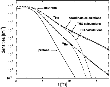
Figure 1: Self-consistent RHB proton and neutron densities for the ground-states of ³⁰Ne and ⁴⁰Ne. Density profiles calculated in THO are compared with FEM. Taken from Stoitsov et al. [64].

2.2.4 Woods-Saxon basis

Woods-Saxon basis from the Schrödinger equation (SWS basis)

For the Schrödinger equation with a spherical Woods-Saxon potential

$$V_{\mathrm{WS}}(r)=\left\{\begin{array}[]{ll}\dfrac{V_{0}}{1+e^{(r-R_{0})/a_{0}}},&r<R_{\mathrm{max}},\\ \infty,&r\geq R_{\mathrm{max}},\\ \end{array}\right.$$ (47)

where $R_{\mathrm{max}}$ is introduced for practical reasons to define the box boundary. The eigenfunction can be written as $\phi_{nlm_{l}}({\mbox{\boldmath${\rm r}$}})=R_{nl}(r)Y_{lm_{l}}(\theta,\phi)$ and its radial Schrödinger equation is derived as

$$\left[-\dfrac{1}{2M}\left(\dfrac{1}{r^{2}}\dfrac{d}{dr}r^{2}\dfrac{d}{dr}-\dfrac{l(l+1)}{r^{2}}\right)+V_{\mathrm{WS}}(r)\right]R_{nl}(r)=\ E_{nl}R_{nl}(r).$$ (48)

Equation (48) is solved on a discretized radial mesh with a mesh size $\Delta r$. $R_{\mathrm{max}}$ ($\Delta r$) is chosen large (small) enough to make sure that the final results do not depend on it. The radial wave functions thus obtained form a complete basis,

$$\left\{R_{nl}(r);n=0,1,\cdots;l=0,1,\cdots,n\right\},$$ (49)

in terms of which the radial part of the upper and the lower components of the Dirac spinor in Eq. (21) are expanded respectively as

$$\left\{\begin{array}[]{l}\displaystyle G_{\alpha}^{\kappa}(r)=-i\sum_{n=0}^{n_{\mathrm{max}}}g_{\alpha n}rR_{nl}(r),\\ \displaystyle F_{\alpha}^{\kappa}(r)=-i\sum_{\tilde{n}=0}^{\tilde{n}_{\mathrm{max}}}f_{\alpha\tilde{n}}rR_{\tilde{n}\tilde{l}}(r).\\ \end{array}\right.$$ (50)

The radial Dirac equation (21) is transformed into the WS basis as

$$\left(\begin{array}[]{cc}{\cal A}_{mn}&{\cal B}_{m\tilde{n}}\\ {\cal C}_{\tilde{m}n}&{\cal D}_{\tilde{m}\tilde{n}}\\ \end{array}\right)\left(\begin{array}[]{c}g_{\alpha n}\\ f_{\alpha\tilde{n}}\\ \end{array}\right)=\epsilon_{\alpha}\left(\begin{array}[]{c}g_{\alpha n}\\ f_{\alpha\tilde{n}}\\ \end{array}\right),$$ (51)

where the matrix elements are calculated as follows

$$\left\{\begin{array}[]{l}\displaystyle{\cal A}_{mn}=\int_{0}^{R_{\mathrm{max}}}r^{2}drR_{ml}(r)\left(V(r)+S(r)+M\right)R_{nl}(r),\\ \displaystyle{\cal B}_{m\tilde{n}}=\int_{0}^{R_{\mathrm{max}}}r^{2}drR_{ml}(r)\left(+\frac{d}{dr}-\frac{\kappa_{\alpha}-1}{r}\right)R_{\tilde{n}\tilde{l}}(r),\\ \displaystyle{\cal C}_{\tilde{m}n}=\int_{0}^{R_{\mathrm{max}}}r^{2}drR_{\tilde{m}\tilde{l}}(r)\left(-\frac{d}{dr}-\frac{\kappa_{\alpha}+1}{r}\right)R_{nl}(r),\\ \displaystyle{\cal D}_{\tilde{m}\tilde{n}}=\int_{0}^{R_{\mathrm{max}}}r^{2}drR_{\tilde{m}\tilde{l}}(r)\left(V(r)-S(r)-M\right)R_{\tilde{n}\tilde{l}}(r).\\ \end{array}\right.$$ (52)

In practical calculations, an energy cutoff $E_{\mathrm{cut}}$ (relative to the nucleon mass $M$) is used to determine the cutoff of the radial quantum number $n_{\mathrm{max}}$ [73].

Woods-Saxon basis from the Dirac equation (DWS basis)

The radial Dirac equation (21) may be solved in $r$ space [68] with Woods-Saxon-like potentials for $V_{0}(r)\pm S_{0}(r)$ [77] within a spherical box of the size $R_{\mathrm{max}}$, together with the spherical spinor which gives a complete WS basis

$$\left\{\left[\epsilon_{n\kappa m}^{0},\psi_{n\kappa m}^{0}({\mbox{\boldmath${\rm r}$}},s,t)\right];\epsilon_{n\kappa m}^{0}\ {}^{<}_{>}\ 0\right\},$$ (53)

with $n=0,1,\cdots$, $\kappa=\pm 1,\pm 2,\cdots$, and $m=-j_{\kappa},\cdots,j_{\kappa}$. $\psi_{n\kappa m}^{0}({\mbox{\boldmath${\rm r}$}},s,t)$ takes the form of Eq. (20). In such cases, states both in the Fermi sea and in the Dirac sea should be included in the basis for completeness. The nucleon wave function (20) can be expanded in terms of this set of basis as

$$\psi_{\alpha\kappa m}({\mbox{\boldmath${\rm r}$}},s,t)=\sum_{n=0}^{n_{\mathrm{max}}}c_{\alpha n}\psi_{n\kappa m}^{0}({\mbox{\boldmath${\rm r}$}},s,t),$$ (54)

where $n_{\mathrm{max}}=n_{\mathrm{max}}^{+}+n_{\mathrm{max}}^{-}+1$ and the summation runs over positive energy levels in the Fermi sea for $0\leq n\leq n_{\mathrm{max}}^{+}$ and over negative energy levels in the Dirac sea for $n_{\mathrm{max}}^{+}+1\leq n\leq n_{\mathrm{max}}$. The negative energy states are obtained with the same method as the positive energy ones. In this WS basis, the Dirac equation (21) turns out to be

$$c_{\alpha m}\epsilon_{m}^{0}+\sum_{n=0}^{n_{\mathrm{max}}}c_{\alpha n}H^{\prime}_{mn}=\epsilon_{\alpha}c_{\alpha m},\ m=1,\cdots,n_{\mathrm{max}},$$ (55)

with

$$H^{\prime}_{mn} = \left\langle\psi_{m}^{0}({\mbox{\boldmath${\rm r}$}})\right|\left[\Delta V({\mbox{\boldmath${\rm r}$}})+\beta\Delta S({\mbox{\boldmath${\rm r}$}})\right]\left|\psi_{n}^{0}({\mbox{\boldmath${\rm r}$}})\right\rangle$$ (56)

$$= \int_{0}^{R_{\mathrm{max}}}drG_{m}^{0}(r)\left[\Delta V(r)+\Delta S(r)\right]G_{n}^{0}(r)$$

$$+ \int_{0}^{R_{\mathrm{max}}}drF_{m}^{0}(r)\left[\Delta V(r)-\Delta S(r)\right]F_{n}^{0}(r),$$

where $\Delta V({\mbox{\boldmath${\rm r}$}})=V({\mbox{\boldmath${\rm r}$}})-V_{0}({\mbox{\boldmath${\rm r}$}})$, $\Delta S({\mbox{\boldmath${\rm r}$}})=S({\mbox{\boldmath${\rm r}$}})-S_{0}({\mbox{\boldmath${\rm r}$}})$ and the angular, spin, and isospin quantum numbers are omitted for brevity.

In the expansion (54) of the nucleon wave function in the SRHDWS theory, one has to take into account not only the states in the Fermi sea but also those in the Dirac sea because these states form a complete basis together. The contribution from negative energy states for ¹⁶O is given in Table 1. It is found that, without including the negative energy levels, the calculated results will depend on the potentials for the basis.

Table 1: Effects of negative energy levels on bulk properties in SRHDWS for ¹⁶O. The effective interaction for the Lagrangian is NLSH, $R_{\rm{max}}=20$ fm, $\Delta r=0.1$ fm, and $N^{+}_{\rm{max}}=25$. For the initial Woods-Saxon like potentials, parameters in Ref. [77] are used except for $V_{0}$ which is specified in the table. The left value in each entry gives the result without negative energy levels included and the right one that with $N^{-}_{\rm{max}}$ = 25. Energy is in MeV and radius in fm. Taken form Ref. [73].

$V_{0}$	$54$ MeV		$72$ MeV		$90$ MeV
$N^{-}_{\rm{max}}$	0	25	0	25	0	25
$E/A$	8.547	8.013	8.117	8.015	8.427	8.012
$r_{\rm rms}$	2.385	2.568	2.531	2.567	2.610	2.567

The contribution of negative energy states in the Dirac sea to the wave function can be calculated by $\sum_{n}|c_{n}^{-}|^{2}$ in the expansion (54) and it is around $10^{-4\sim-5}$ (Note that the nucleon wave function is normalized to one). However, such a small component from negative energy states in the wave functions contributes to the physical observables such as $E/A$ and $r_{\rm{rms}}$ by magnitudes of 1$\sim$10 % as can be seen from Table 1.

Comparisons between $r$ space, harmonic oscillator basis and Woods-Saxon basis

It is found that for stable nuclei, the SRHR, SRHSWS, SRHDWS, and SRHHO approaches are all valid and results from them are in excellent agreement with each other [73]. However, for unstable nuclei near the neutron drip line, these methods differ from each other to some extent.

In Fig. 2, the neutron density distribution of ⁷²Ca from different SRH approaches are compared. With the same box size, the density distribution from SRHR are almost identical with those from SRHWS, which indicates the equivalence between SRHWS and SRHR. For brevity, only $\rho_{\rm n}(r)$ from SRHR with $R_{\rm max}$ = 35 fm is displayed which covers the curve corresponding to $\rho_{n}(r)$ from SRHWS with $R_{\rm max}$ = 35 fm in Fig. 2. On the other hand, $\rho_{\rm n}(r)$ from SRHHO even with $N_{\rm max}$ = 43 fails to reproduce the result of SRHR due to the well known localization property of HO potential [64].

These results indicate that even the long tail (or halo) behavior in neutron density distribution for nuclei near the drip line can be reproduced quite well by the expansion method in the Woods-Saxon basis in the Schrödinger framework (SRHSWS) and that in the Dirac framework (SRHDWS). This can be seen that the neutron density distribution obtained in SRHR is reproduced well in both SRHSWS and SRHDWS when enough box size is taken.

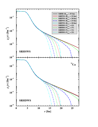
Figure 2: Comparison of density distributions for ⁷²Ca from SRHR, SRHWS and SRHHO with NLSH. $\Delta r$ = 0.1 fm for SRHR and SRHWS. $E_{\rm cut}$ = 75 MeV and $R_{\rm max}$ = 20 (thick dot-dashed curve), 25 (thick long-dashed curve), 30 (thick dashed curve) and 35 fm (thick dotted curve) for SRHWS. These sets of cutoff’s correspond to cutoff’s in principal quantum number $N_{\rm max}$ = 25 (thin dot-dashed curve), 31 (thin long-dashed curve), 37 (thin dashed curve) and 43 (thin dotted curve) which are used in SRHHO calculations. Taken form Ref. [73].

2.3 Effective interactions

In the Lagrangian density (1), there are meson masses $m_{\sigma},m_{\omega},m_{\rho}$ and meson-nucleon coupling constants $g_{\sigma},g_{\omega},g_{\rho}$ together with the nonlinear self-couplings of the meson fields left to be determined. They are the nucleon-nucleon interactions in the RMF theory and in principle should be determined either by more fundamental theories or by experiments. However, as the relativistic mean field theory is formulated on the basis of the above effective Lagrangian in connection with the mean-field and the no-sea approximations, it is difficult to determine these interactions microscopically. Instead, the masses and coupling strengthes of the mesons and the nonlinear self-couplings of the meson fields are determined by reproducing the properties of nuclear matter and a few doubly magic nuclei. Namely, they are effective interactions in the similar sense as their conventional counterparts. The effective interactions in the RMF theory could be determined by minimizing the least square error as follows,

$$\chi^{2}({\mbox{\boldmath${\rm a}$}})=\sum_{i=1}^{N}\left[\frac{y^{exp}_{i}-y(x_{i};{\mbox{\boldmath${\rm a}$}})}{\sigma_{i}}\right]^{2},$$ (57)

where ${\rm a}$ is the ensemble of the meson masses $m_{\sigma},m_{\omega},m_{\rho}$ and the meson-nucleon coupling constants $g_{\sigma},g_{\omega},g_{\rho}$ together with the nonlinear self-couplings of the meson fields to be fitted, and $y^{exp}_{i}$ and $\sigma_{i}$ are the experimental observables and corresponding weights. In general, the masses and charge radii of spherical nuclei near the $\beta$-stability line are adopted as observables in the least-square fitting procedure.

Among the existing effective interactions for the RMF theory, the most frequently used are NL1 [78], NLSH [79], TM1 [50] and NL3 [80] with nonlinear self-couplings of mesons. Along the $\beta$-stability line NL1 gives excellent results for binding energies and charge radii, in addition it provides an excellent description of the superdeformed bands  [81, 82]. However, when moving away from the stability line the results are less satisfactory. This can be partly attributed to the large asymmetry energy $J\simeq$ 44 MeV. Moreover, the neutron skin thicknesses calculated with NL1 show systematic deviations from the experimental data [83].

In NLSH this problem was treated in a better way and the improved isovector properties have been obtained with an asymmetry energy of $J\simeq$ 36 MeV. Furthermore, NLSH seems to describe the deformation properties in a better way than NL1 does. However, NLSH produces a slight over-binding along the line of $\beta$-stability and in addition it fails to reproduce successfully the superdeformed minima in Hg-isotopes in constrained calculations for the energy landscape. A remarkable difference between the two effective interactions are the quite different values predicted for the nuclear matter incompressibility  [84], i.e., $K$ = 212 MeV for NL1 while $K$ = 355 MeV for NLSH [85, 86]. As an improvement, NL3 and TM1 provide reasonable compression modulus ($K_{\text{NL3}}=271.7\ \text{MeV},K_{\text{TM1}}=281.16\ \text{MeV}$) and asymmetry energy ($J_{\text{NL3}}=37.42\ \text{MeV},J_{\text{TM1}}=36.89\ \text{MeV}$) but fairly small baryonic saturation density ($\rho_{\text{TM1}}=0.145$). In order to improve the description of these quantities, two nonlinear self-coupling effective interactions, PK1 with nonlinear $\sigma$- and $\omega$-meson self-couplings and PK1R with nonlinear $\sigma$-, $\omega$- and $\rho$-meson self-couplings were developed [51] (see Table 3).

In order to reproduce better the experimental quantities such as the binding energies and nuclear radii, etc., an additional correction should be added in calculating the energy, i.e., the center-of-mass correction. Conventionally a phenomenological center-of-mass correction as $-\dfrac{3}{4}\,41A^{-1/3}$ is used. Microscopically the correction can be calculated by the projection-after-variation in first-order approximation [87]:

$$E^{\text{mic.}}_{\text{c.m.}}=-\frac{1}{2MA}\left<{{\mbox{\boldmath${\rm P}$}}}_{\text{c.m.}}^{2}\right>,$$ (58)

where the center-of-mass momentum ${\mbox{\boldmath${\rm P}$}}_{\text{c.m.}}=\sum_{i}^{A}{\mbox{\boldmath${\rm p}$}}_{i}$ and the expectation value of its square $\left<{\mbox{\boldmath${\rm P}$}}_{\text{c.m.}}^{2}\right>$ reads

$$\left<{{\mbox{\boldmath${\rm P}$}}}_{\text{c.m.}}^{2}\right>=\sum_{a}v_{a}^{2}p_{aa}^{2}-\sum_{a,b}v_{a}^{2}v_{b}^{2}{\mbox{\boldmath${\rm p}$}}_{ab}\cdot{\mbox{\boldmath${\rm p}$}}^{*}_{ab}+\sum_{a,b}v_{a}u_{a}v_{b}u_{b}{\mbox{\boldmath${\rm p}$}}_{ab}\cdot{\mbox{\boldmath${\rm p}$}}_{\bar{a}\bar{b}}$$ (59)

with occupation probabilities $v_{a}^{2}$ and $u_{a}^{2}=1-v_{a}^{2}$ accounting for the pairing effects, where $a,b$ denote the BCS states (see the following section).

Here it should be mentioned that the prescription (58) is based on non-relativistic considerations. It does not preserve Lorentz invariance. Furthermore, it also breaks the complete self-consistence of the variational scheme. However, as it is not included in the self-consistent procedure and only presents an additional correction term to the binding energy, one can be satisfied with it for the moment. Compared with the binding energy, this center-of-mass correction is sizable in light nuclei (about 9% in ¹⁶O) but much less important in medium and heavy nuclei (about 0.4% in ²⁰⁸Pb) as seen in Fig. 3.

Figure 3: The microscopic center-of-mass correction in comparison with two phenomenological cases. Taken from Ref. [51].

Table 2: The nonlinear effective interactions PK1, PK1R and density-dependent effective interaction PKDD  [51] in comparison with TM1 [50], NL3 [80], TW99 [61], and DD-ME1 [62].

	PK1	PK1R	PKDD	TM1	NL3	TW99	DD-ME1
$M_{n}$	939.5731	939.5731	939.5731	938	939	939	938.5000
$M_{p}$	938.2796	938.2796	938.2796	938	939	939	938.5000
$m_{\sigma}$	514.0891	514.0873	555.5112	511.198	508.1941	550	549.5255
$m_{\omega}$	784.254	784.2223	783	783	782.501	783	783.0000
$m_{\rho}$	763	763	763	770	763	763	763.0000
$g_{\sigma}$	10.3222	10.3219	10.7385	10.0289	10.2169	10.7285	10.4434
$g_{\omega}$	13.0131	13.0134	13.1476	12.6139	12.8675	13.2902	12.8939
$g_{\rho}$	4.5297	4.55	4.2998	4.6322	4.4744	3.661	3.8053
$g_{2}$	$-$8.1688	$-$8.1562	0	$-$7.2325	$-$10.4307	0	0.0000
$g_{3}$	$-$9.9976	$-$10.1984	0	0.6183	$-$28.8851	0	0.0000
$c_{3}$	55.636	54.4459	0	71.3075	0	0	0.0000
$d_{3}$	0	350	0	0	0	0	0

Table 3: Density-dependent parameters of PKDD [51] for meson-nucleon couplings in comparison with TW99 [61] and DD-ME1 [62].

	$a_{\sigma}$	$b_{\sigma}$	$c_{\sigma}$	$d_{\sigma}$	$a_{\omega}$	$b_{\omega}$	$c_{\omega}$	$d_{\omega}$	$a_{\rho}$
PKDD	1.327423	0.435126	0.691666	0.694210	1.342170	0.371167	0.611397	0.738376	0.183305
TW99	1.365469	0.226061	0.409704	0.901995	1.402488	0.172577	0.344293	0.983955	0.515000
DD-ME1	1.3854	0.9781	1.5342	0.4661	1.3879	0.8525	1.3566	0.4957	0.5008

For the nuclear radii, the effects from the center-of-mass motion can also be taken into account as follows. Because of its fairly small effects, a rather rough correction is adopted for protons,

$$\delta R_{p}^{2}=-\frac{2}{Z}\sum_{a}^{A}\left<\phi_{a}\right|{\mbox{\boldmath${\rm R}$}}_{\text{c.m.}}\cdot\sum_{i}^{Z}{\mbox{\boldmath${\rm r}$}}_{i}\left|\phi_{a}\right>+\sum_{a}^{A}\left<\phi_{a}\right|{\mbox{\boldmath${\rm R}$}}_{\text{c.m.}}^{2}\left|\phi_{a}\right>,$$ (60)

where the center-of-mass coordinate ${\mbox{\boldmath${\rm R}$}}_{\text{c.m.}}=1/A\sum_{i}^{A}{\mbox{\boldmath${\rm r}$}}_{i}$. Then one obtains,

$$\delta R_{p}^{2}=-\frac{2}{A}R_{p}^{2}+\frac{1}{A}R_{M}^{2},$$ (61)

where $R_{p}$ and $R_{M}$ denote the proton and matter radii. Here we only consider the direct-term contributions to Eq. (60) to conform to the spirit of the RMF theory. For the neutron radii, one can follow the same procedure as that for protons. The charge radius is obtained from the proton radius combining with the proton and neutron size and the center-of-mass correction (61) included in $R_{p}^{2}$ [50]

$$R_{\text{ch}}^{2}=R_{p}^{2}+(0.862\ \text{fm})^{2}-(0.336\ \text{fm})^{2}N/Z.$$ (62)

With the microscopic center-of-mass motion, a multi-parameter fitting can be performed using the Levenberg-Marquardt method [88]. In Ref. [51], the masses of ¹⁶O, ⁴⁰Ca, ⁴⁸Ca, ⁵⁶Ni, ⁶⁸Ni, ⁹⁰Zr, ¹¹⁶Sn, ¹³²Sn, ¹⁹⁴Pb and ²⁰⁸Pb and the bulk quantities of nuclear matter are chosen as observables to determine the effective interactions. The radii are excluded because the proper values of the compression modulus $K$ and the baryonic saturation density $\rho_{0}$ are sufficient to give a good description of the radii. For a fixed value of the compression modulus $K$, a large baryonic saturation density $\rho_{0}$ will give a small charge radius and vice versa. Therefore a proper description of both masses and radii of finite nuclei could be obtained by carefully adjusting the values of these two quantities $K$ and $\rho_{0}$. To give a fairly precise description of the masses, the center-of-mass correction is also essential for both light and heavy nuclei. As it can be seen in Fig. 3, the deviation between the microscopic and phenomenological results is considerably large not only for the light nuclei but also for the heavy ones. And there exist very remarkable shell effects in the microscopic results which are impossible to obtain with the phenomenological methods. The microscopic center-of-mass correction [87], therefore, is chosen to deal with the center-of-mass motion.

Because the contribution to the nuclear masses from the nonlinear $\rho$-meson term is found to be fairly small, the effective interaction PK1R is obtained by fixing the nonlinear self-coupling constant $d_{3}$ to 350.0 and adjusting other parameters.

In the RMF theory with density-dependent meson-nucleon couplings, the density-dependence of the coupling constants $g_{\sigma}$ and $g_{\omega}$ can be parameterized as,

$$g_{i}(\rho_{v})=g_{i}(\rho_{\text{sat}})f_{i}(x)~{}~{}~{}~{}~{}~{}~{}~{}\text{ for }i=\sigma,\omega,$$ (63)

where

$$f_{i}(x)=a_{i}\frac{1+b_{i}(x+d_{i})^{2}}{1+c_{i}(x+d_{i})^{2}}$$ (64)

is a function of $x=\rho_{v}/\rho_{\text{sat}}$, and $\rho_{\text{sat}}$ denotes the baryonic saturation density of nuclear matter. For the $\rho$ meson, an exponential dependence is utilized as

$$g_{\rho}=g_{\rho}(\rho_{\text{sat}})\exp[-a_{\rho}(x-1)].$$ (65)

For the functions $f_{i}(x)$, one has five constraint conditions $f_{i}(1)=1,f_{\sigma}^{\prime\prime}(1)=f_{\omega}^{\prime\prime}(1)$ and $f_{i}^{\prime\prime}(0)=0$. Then 8 parameters related to density dependence for $\sigma$-N and $\omega$-N couplings are reduced to 3 free parameters. In general, the masses of the nucleons and the $\rho$-meson are fixed and the nonlinear self-coupling constants $g_{2},g_{3},c_{3}$ and $d_{3}$ are set to zero. With 4 free parameters for density dependence, totally there are 8$\sim$9 parameters left free in the Lagrangian density (1) for the density-dependent meson-nucleon coupling RMF theory. A density-dependent meson-nucleon coupling effective interaction PKDD has also been obtained in Ref. [51] (see Tables 3 and 3).

Tables 3 and 3 tabulate the new effective interactions PK1, PK1R and PKDD [51] in comparison with the old ones TM1 [50], NL3 [80], TW99 [61] and DD-ME1 [62]. The newly obtained ones reproduce better the experimental masses [89]. PK1, PK1R and PKDD also describe the charge radii very well, especially for those of the Pb isotopes. More comprehensive comparisons between Hartree-Fock-Bogoliubov, extended Thomas-Fermi model with Strutinski integral, RMF, and macroscopic-microscopic approaches with different forces have been performed for the description of nuclear masses and charge radii of spherical even-even nuclei (116 nuclides), from light (A=16) to heavy (A=220) ones in Ref. [90].

Table 4 lists the nuclear matter quantities calculated with the newly obtained effective interactions PK1, PK1R and PKDD, in comparison with those from the other interactions. All the new effective interactions give a proper value for the compression modulus $K$.

Table 4: Nuclear matter properties calculated with PK1, PK1R and PKDD [51] in comparison with those with TM1 [50], NL3 [80], TW99 [61], DD-ME1 [62].

Interaction	$\rho_{\text{sat.}}(\text{fm}^{-3})$	$E_{b}$ [MeV]	K [MeV]	$J$ [MeV]	$M^{*}/M$(n)	$M^{*}/M$(p)
PK1	0.1482	$-$16.268	282.644	37.641	0.6055	0.6050
PK1R	0.1482	$-$16.274	283.674	37.831	0.6052	0.6046
PKDD	0.1496	$-$16.267	262.181	36.790	0.5712	0.5706
NL3	0.1483	$-$16.250	271.729	37.416	0.5950	0.5950
TM1	0.1452	$-$16.263	281.161	36.892	0.6344	0.6344
TW99	0.1530	$-$16.247	240.276	32.767	0.5549	0.5549
DD-ME1	0.1520	$-$16.201	244.719	33.065	0.5780	0.5780

2.4 Density and isospin dependence of effective interactions

There are so far quite a number of effective interactions, PK1, PK1R, PKDD [51] together with NL1, NL2 [91], NL3 [80], NLSH [79], TM1, TM2 [50], GL-97 [92] and the density-dependent effective interactions TW-99 [61], DD-ME1 [62], etc.. It is very interesting to investigate the density and isospin dependence of the interaction strengthes of various effective interactions in the RMF theory and study their effects on nuclear matter [93]. Although for the nonlinear self-coupling effective interactions, the density dependencies are only embodied in the Klein-Gordon equations, it is still worthwhile to obtain a quantitative understanding of the coupling constants.

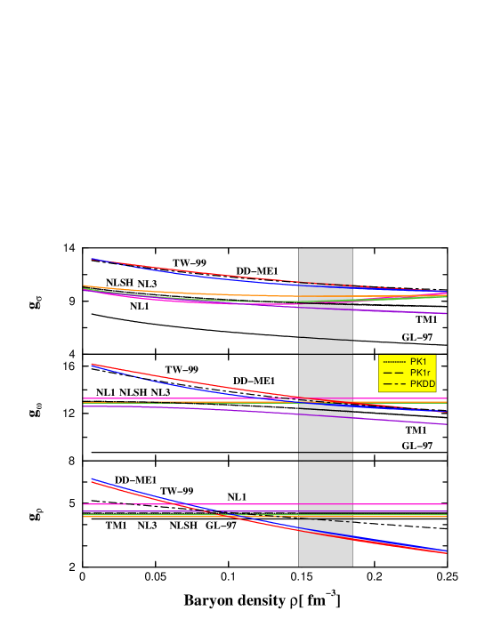
Figure 4: Density dependence of the interaction strengths for $g_{\sigma}$(top), $g_{\omega}$(middle) and $g_{\rho}$(bottom) in nuclear matter as functions of the nuclear density. The shadowed area corresponds to the empirical value of saturation point in nuclear matter (Fermi momentum $k_{F}=1.35\pm 0.05$ fm^-1 or density $\rho=0.166\pm 0.018$ fm^-3). Taken from Ref. [51].

In Fig. 4, the density dependencies of the interaction strengthes for $g_{\sigma}$(top), $g_{\omega}$(middle) and $g_{\rho}$(bottom) in nuclear matter as functions of the nuclear density are shown. The curves in the figures from top to bottom are labelled in the order of from left to right. The shadowed area corresponds to the empirical value of the saturation point in nuclear matter, i.e., Fermi momentum $k_{F}=1.35\pm 0.05$ fm^-1 or density $\rho=0.166\pm 0.018$ fm^-3. For the nonlinear effective interactions, the “equivalent” density dependence of the interaction strengthes for $\sigma$, $\omega$ and $\rho$ is extracted from the meson field equations according to [51]:

$$g_{\sigma} \sim g_{\sigma}+\left[g_{2}\sigma^{2}+g_{3}\sigma^{3}\right]/\rho_{s},$$ (66a)

$$g_{\omega} \sim g_{\omega}-c_{3}\omega_{0}^{3}/\rho_{v},$$ (66b)

$$g_{\rho} \sim g_{\rho}-d_{3}({\rho_{0}^{3}})^{3}/{\rho_{3}}.$$ (66c)

For the $\sigma$-meson, TW-99 and DD-ME1 exhibit quite different behaviors for $g_{\sigma}$ compared with those of the other effective interactions in either magnitude or slope. In particular, the strengthes in TW-99 and DD-ME1 for the density interval in Fig. 4 are almost two times larger than that of GL-97. Quite different results can also be seen at the empirical nuclear matter densities. For the $\omega$-meson, except for TW-99, DD-ME1, TM1, and GL-97, the strengthes in all the other effective interactions are density-independent. However, the strengthes are closer to each other at the empirical saturation density than those of the $\sigma$-meson although large differences can also be seen at low densities. For the $\rho$-meson which describes the isospin asymmetry, the strengthes for TW-99 and DD-ME1 show strong density dependence in contrast with those of the other effective interactions; while those of PK1, PK1R and PKDD are just in between [51].

In Fig. 5, the behavior of the binding energy per particle $E/A$ as a function of the baryonic density $\rho$ is shown for symmetric nuclear matter (left) and neutron matter (right). It is seen that all the density-dependent meson-nucleon coupling effective interactions give softer results than the nonlinear self-coupling ones , especially for neutron matter. The behaviors predicted by PK1, PK1R are much softer than that by NL3 and a little harder than that by TM1. The results from PKDD are slightly softer than that from DD-ME1 and much harder than that from TW99 at high densities. All these behaviors can be explained in the density-dependent meson-nucleon coupling framework.

As what have been mentioned in expressions (66), the meson-nucleon coupling constants in the nonlinear self-coupling of mesons can be expressed as some kind of density-dependence. Fig. 4 shows the density-dependence of the coupling constants for the nonlinear self-coupling effective interactions and for the density-dependent version, where almost all the density-dependent coupling constants decrease with increasing density except for $g_{\sigma}$ of NL3, NLSH, NL1, which has strong $\sigma^{4}$ self-couplings. On the other hand, the coupling constants $g_{\sigma}$ and $g_{\omega}$ of TM1, which has relatively weak $\sigma$ self-coupling ($g_{3}=0.6183$) and strong $\omega$ self-coupling ($c_{3}=71.3075$), are smaller than the others, which means that TM1 provides relatively weaker scalar and vector potentials. This is the reason why TM1 presents the softer behavior than the other nonlinear self-coupling effective interactions. In Fig. 5, TW99 predicts the softest results because of its relatively small $g_{\omega}$ as compared with DD-ME1, PKDD and NL3, and large $g_{\sigma}$ as compared with PK1, PK1R and TM1 in Fig. 4. As it is known, the repulsive potential would be dominant at high densities. In Fig. 5, NL3 gives the hardest results because of its constant and large $g_{\omega}$ even though its $\sigma$-N coupling constant $g_{\sigma}$ increases with the density. For PK1, PK1R and PKDD, which present the mid soft behaviors in Fig.5, the coupling constants also lie between the largest and the smallest in Fig. 4. There exists a significant difference between symmetric nuclear matter and neutron matter. The density-dependent effective interactions PKDD and DD-ME1 present similar trends as PK1, PK1R and TM1 in symmetric nuclear matter but much softer in neutron matter, which may be interpreted by the density-dependence of $g_{\rho}$. For the effective interaction PK1R, the density-dependence of the $g_{\rho}$ is fairly weak as compared with that of the density-dependent meson-nucleon coupling effective interactions. It can be explained by a very weak $\rho$-field, which generates neutron-proton asymmetry field. The behavior of $g_{\rho}$ with respect to the neutron-proton ratio is shown in Fig.6. As expected, the behavior is symmetric with respect to $\ln(N/Z)$ and the density-dependence becomes more remarkable with the increase of the baryonic density and the neutron-proton asymmetry.

Figure 5: The energy per particle $E/A$ in symmetric nuclear matter (left) and neutron matter (right) as functions of the baryon density $\rho$. The shaded area indicates the empirical saturation region. The filled diamond presents the data taken from Ref. [94] as comparison.

Figure 6: The density-dependence of $g_{\rho}$ for PK1R with respect to the neutron-proton ratio N/Z. Taken from Ref. [51].

3 Relativistic continuum Hartree-Bogoliubov theory

Pairing correlations are due to the short range part of the nucleon-nucleon interaction and play important roles in open shell nuclei. A simple and commonly used method of dealing with pairing correlations is the BCS approach under the constant gap approximation. The BCS method can be combined easily with the relativistic mean field theory as shown in Refs. [78, 21]. However, the conventional BCS method is not justified for exotic nuclei because it could not include properly the contribution of continuum states. Bogoliubov transformation is the generalization of the BCS scheme. By quantizing the meson field and making Gorkov factorization, the relativistic Hartree Bogoliubov (RHB) formalism was derived [95]. In order to describe the exotic nuclei, the relativistic continuum Hartree Bogoliubov (RCHB) theory was developed, in which the continuum states are discretized and the RHB equations are solved in the coordinate space [36, 42].

In this section, the pairing correlations, the conventional BCS approach, the continuum states, the resonant BCS method and several methods for obtaining single particle resonant states are briefly reviewed. Finally, the detailed formalism of the RCHB theory together with the discussion on the effective pairing interactions are given.

3.1 Pairing correlations

3.1.1 BCS approximation

For Fermion systems like atomic nuclei, Kramers degeneracy ensures the existence of pairs of degenerate, mutually time-reversal conjugate states, which could be coupled strongly by a short-range force, namely a $pp$-channel in the framework of mean field. Physically, such pairing correlations lead to the superfluidity. In Hartree approximation, the ground state properties could be described by filling the single particle levels from the bottom up to the Fermi level. The occupation probability of each single particle level is either zero or one. Due to pairing interaction, pairs of nucleons are scattered from the levels below the Fermi level to those above. Thus for the open shell nuclei, one has to deal with the occupation probabilities ranging from zero to one. Mathematically, this could be treated by introducing the concept of quasi-particles. For stable nuclei, the pairing gap can be extracted from the experimental odd-even mass difference and the BCS approximation is very simple and useful. For $M$-single particle orbitals in the Hartree approximation, for each particle orbital $k$ ($k=1,\cdots,M$), one can introduce the quasi-particle energy:

$$E_{k}=\left[(\epsilon_{k}-\lambda)^{2}+\Delta^{2}\right]^{1/2},$$ (67)

and the corresponding occupation probability:

$$v_{k}^{2}=\dfrac{1}{2}\left[1-\dfrac{\epsilon_{k}-\lambda}{E_{k}}\right],$$ (68)

where $\lambda$ is the Fermi level determined by the particle number $N=\displaystyle\sum_{k=1}^{M}v_{k}^{2}$ and $\Delta$ the pairing gap determined from the experimental odd-even mass difference

$$\Delta=\frac{1}{2}\left[E(N+2)-E(N+1)-(E(N+1)-E(N))\right],$$ (69)

or deduced from certain pairing Hamiltonian $H_{\rm pair}$ when the experimental binding energies are unknown. For monopole pairing interaction $H_{\rm pair}=G\displaystyle\sum_{kk^{\prime}>0}a_{k}^{+}a_{\bar{k}}^{+}a_{\bar{k}^{\prime}}a_{k^{\prime}}$, there lies the pairing gap equation with classical variation:

$$\Delta=G\sum_{k>0}u_{k}v_{k}=\frac{G}{2}\sum_{k>0}\frac{\Delta}{E_{k}},$$ (70)

where $u_{k}$ satisfies $u_{k}^{2}=1-v_{k}^{2}$. For fixed values of the gap parameters $\Delta$ or pairing interaction strengthes $G$ for neutrons and protons, the self-consistent solution is obtained by iteration.

The BCS method can be easily implemented into the relativistic mean field description with the single particle orbitals in the relativistic Hartree level. However, it is only valid for bound states. For the extremely neutron-rich (or proton-rich) nuclei near the drip lines, the continuum states begin to contribute as schematically shown in Fig. 7. The conventional BCS approach will involve unphysical states and lead to the divergence. For these nuclei, one must either investigate the detailed properties of continuum states and include the coupling between the bound state and the continuum by extending the BCS method to resonant BCS theory (see Section 3.2.2) or generalize the BCS model by unifying the Hartree (or Hartree-Fock) scheme and the Bogoliubov transformation (see Section 3.3).

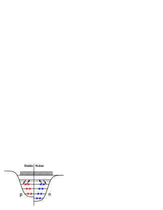
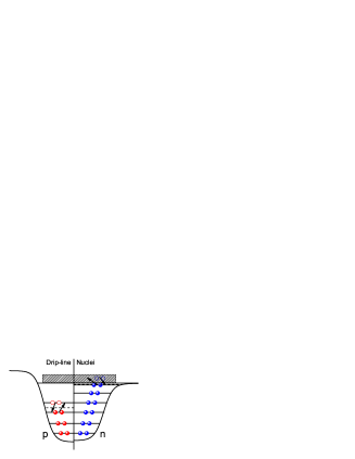
Figure 7: The schematic picture for the difference in the pairing correlation of stable and drip line nuclei. Normally the last filled nucleon in stable nuclei has $8$ MeV binding, while it is near the threshold in drip line nuclei. The pairing correlation in exotic nuclei provides the possibility to scatter valence nucleons back and forth in the continuum.

3.2 Continuum states

3.2.1 Single particle resonant states

For stable open shell nuclei, the pairing gaps are of the order of MeV [16]. There are some evidences that the pairing gaps will increase towards the drip lines. For nuclei close to drip lines, the one or two particle separation energies are usually very small. For example, the one proton separation energies $S_{p}$ are 0.138 MeV, 0.60 MeV and 0.29 MeV in ⁸B, ¹²N and ³¹Cl; the two neutron separation energies $S_{2n}$ are 0.30 MeV and 1.33 MeV in ¹¹Li and ¹⁴Be [89]. A small particle separation energy means that the Fermi level is very close to the threshold. Therefore, pairing correlations can scatter valence nucleons between bound and continuum states as seen from Fig. 7. An unphysical continuum state distributes over the whole space while a physical resonance state with positive energy stays inside the nucleus for a long time and has better asymptotic behavior. For the cases where the pairing correlations involve the continuum, such as exotic nuclei, it has been demonstrated that the largest contribution to the pairing correlations is expected to come from the resonant continuum part [37, 36, 42, 96, 97, 41]. Therefore it’s very important to investigate single particle resonant states in exotic nuclei.

Various techniques have been developed to study resonant states in the continuum such as the R-matrix theory [98] and the extended R-matrix theory [99], the K-matrix theory [100] and the conventional scattering theory [101]. By discretizing the continuum, the contribution of the resonant states can be self-consistently taken into account via a Bogoliubov transformation in coordinate space [37, 36, 42]. The bound-state-type methods have also been developed, including the real stabilization method [102], the complex scaling method (CSM) [103], and the analytic continuation in the coupling constant (ACCC) method [104]. Within the framework of the non-relativistic Schrödinger equation, the ACCC method has been applied to investigate the energies and widths for resonant states in light nuclei combined with few-body methods [105, 106], and to study single-particle resonant states in spherical and deformed nuclei by solving the Schrödinger equation with Woods-Saxon potentials [107]. Recently the ACCC method and phase shift scattering method have been combined with the RMF model.

The philosophy of the ACCC method is that a resonant state becomes a bound one if one increases the attractive potential. Then the energy, width, and wave function of the resonant state can be obtained by an analytic continuation carried out via a Pad$\acute{\text{e}}$ approximant (PA) from the bound-state solutions. Compared with other bound-state-type methods, the ACCC approach is very effective and numerically quite simple because many methods available for bound-state problems can be used and the PA for analytic continuation can be implemented in easily.

By solving the spherical relativistic Hartree equations in a meshed box of size $R_{0}$ self-consistently, one can calculate the ground state properties of a nucleus. The vector potential $V(r)$ and the scalar potential $S(r)$, energies and wave functions for bound states are also obtained. By increasing the attractive potential $(V(r)+S(r))$ to $\lambda(V(r)+S(r))$ , a resonant state will be lowered and becomes bound if the coupling constant $\lambda$ is large enough. Near the branch point $\lambda_{0}$, defined by the scattering threshold $k(\lambda_{0})=0$ [104], the wave number $k(\lambda)$ behaves as

$$k(\lambda)\sim\left\{\begin{array}[]{l@{\mbox{~~~}}l}i\sqrt{\lambda-\lambda_{0}},\hfil\mbox{~{}~{}~{}&l>0,\\ i(\lambda-\lambda_{0}),\hfil\mbox{~{}~{}~{}&l=0.\end{array}\right.}}$$ (73)

These properties suggest an analytic continuation of the wave number $k$ in the complex $\lambda$ plane from the bound-state region into the resonance region by Pad$\acute{\text{e}}$ approximant of the second kind (PAII) [104]

$$k(x)\approx k^{[L,N]}(x)=i\dfrac{c_{0}+c_{1}x+c_{2}x^{2}+\ldots+c_{L}x^{L}}{1+d_{1}x+d_{2}x^{2}+\ldots+d_{N}x^{N}},$$ (74)

where $x\equiv\sqrt{\lambda-\lambda_{0}}$, and $c_{0},c_{1},\ldots,c_{L},d_{1},d_{2},\ldots,d_{N}$ are the coefficients of PA. These coefficients can be determined by a set of reference points $x_{i}$ and $k(x_{i})$ obtained from the Dirac equation with $\lambda_{i}>\lambda_{0},~{}i=1,2,...,L+N+1$. With the complex wave number $k(\lambda=1)=k_{r}+ik_{i}$, the resonance energy $E$ and the width $\Gamma$ can be extracted from the relation $\varepsilon=E-i\dfrac{\Gamma}{2}~{}~{}(E,\Gamma\in\mathbb{R})$ and $k^{2}=\varepsilon^{2}-M^{2}$, i.e.,

$$E = \sqrt{\dfrac{\sqrt{(M^{2}+k_{r}^{2}-k_{i}^{2})^{2}+4k_{r}^{2}k_{i}^{2}}+(M^{2}+k_{r}^{2}-k_{i}^{2})}{2}}-M,$$

$$\Gamma = \sqrt{2\sqrt{(M^{2}+k_{r}^{2}-k_{i}^{2})^{2}+4k_{r}^{2}k_{i}^{2}}-2(M^{2}+k_{r}^{2}-k_{i}^{2})}.$$ (75)

Based on the Schrödinger and Dirac equations, the stability and convergence of the energies and widths for single-particle resonant states with square-well, harmonic-oscillator and Woods-Saxon potentials have been investigated and their dependence on the coupling constant interval and the order of the PA have been discussed [108, 109]. Combined with the RMF theory, the ACCC method was employed to study energies and widths for resonant states in stable nuclei ¹⁶O and ⁴⁸Ca in Ref. [110] and to explore the single-particle resonant states, including resonance parameters and wave functions, in exotic nuclei in Ref. [111].

The continuation in the coupling constant can be replaced by the continuation in $k$ plane along the $k(\lambda)$ trajectory determined by Eq. (74) to the point $k_{R}$ corresponding to the wave number for Gamow state, i.e., $k_{R}=k^{[L,N]}(\lambda=1)$ [104]. Similarly, the wave function $\varphi(k_{R},r)$ for a resonant state can be obtained by an analytic continuation of the bound-state wave function $\varphi(k_{i},r)$ in the complex $k$ plane. One can also prove that the wave function $\varphi(k,r)$ is an analytic function of the wave number $k$ in the inner region $r<R_{0}$ where the Jost function analyticity dominates [104]. Therefore, the technique, which has been adopted to find the complex resonance energy, has been used to determine the resonance wave function $\varphi(k_{R},r)$. Firstly, the PA are constructed to define the resonance wave function at any point $r$ in the inner region ($r<R_{0}$) [104]

$$\varphi^{[L,N]}(k,r)=\dfrac{P_{L}(k,r)}{Q_{N}(k,r)}=\dfrac{a_{0}(r)+a_{1}(r)k+a_{2}(r)k^{2}+\ldots+a_{L}(r)k^{L}}{1+b_{1}(r)k+b_{2}(r)k^{2}+\ldots+b_{N}(r)k^{N}},$$ (76)

where the coefficients ${a_{i}(r)}~{}(i=0,1,\ldots,L)$ and ${b_{j}(r)}~{}(j=1,2,\ldots,N)$ are dependent on $r$. These coefficients can be determined by a set of reference points $k_{i}$ and $\varphi(k_{i},r)$ obtained from the Dirac equation with $\lambda_{i}>\lambda_{0},~{}(i=1,2,...,L+N+1)$. The resonance wave function $\varphi(k_{R},r)=\varphi^{[L,N]}(k_{R},r)~{}(r<R_{0})$ can be extrapolated in this way.

The Dirac equation can be rewritten as two decoupled Schrödinger-like equations for the upper and the lower components respectively [32]. For neutrons, the Schrödinger-like equation for the upper component reads

$$\dfrac{d^{2}G_{i}^{lj}(r)}{dr^{2}}-\dfrac{\kappa_{i}(\kappa_{i}+1)}{r^{2}}G_{i}^{lj}(r)+(E_{i}^{2}-M^{2})G_{i}^{lj}(r)=0,$$ (77)

in the outer region where $V(r)\simeq 0$ and $S(r)\simeq 0$. Its solution is the well known Riccati-Hankel function

$$\hat{h}^{\pm}_{\kappa}(z)=\hat{n}_{\kappa}(z)\pm i\hat{j}_{\kappa}(z),~{}~{}~{}~{}~{}z=kr,$$ (78)

where $\hat{j}_{\kappa}(z)=z{j}_{\kappa}(z)$ is the usual regular solution, i.e. Riccati-Bessel function, and $\hat{n}_{\kappa}(z)=z{n}_{\kappa}(z)$ is the irregular solution, i.e. Riccati-Neumann function. The outer wave function is matched to the inner wave function at $r=r_{m}<R_{0}$

$$\varphi^{[L,N]}(k_{R},r_{m})=C(k_{R})\left[\hat{j}_{\kappa}(k_{R}r_{m})+D(k_{R})\hat{n}_{\kappa}(k_{R}r_{m})\right],$$ (79)

where $C(k_{R})$ is the coefficient for matching and $D(k_{R})=\tan\delta_{\kappa}(k_{R})$ with $\delta_{\kappa}(k_{R})$ the phase shift. It has been found that $\delta_{\kappa}(k_{R})$ is almost a constant when $r_{m}$ is large enough. Given the upper component, the lower component $F_{\kappa}(r)$ can be calculated from the relationship between the upper and the lower components and the resonance wave function is finally normalized according to the Zel’dovich procedures [104]. The wave function for the neutron resonant state $\nu 1g_{9/2}$ in ⁶⁰Ca with different matching points is given in Fig. 8 where one finds the convergence of the wave function with respect to the matching point $r_{m}$ when $r_{m}$ changes from 14 fm to 18 fm.

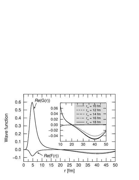
Figure 8: Real parts of the upper and lower components of the radial wave function for the neutron $\nu 1g_{9/2}$ state in ⁶⁰Ca calculated by the ACCC method with different matching points $r_{m}$. Taken from Ref. [111].

The resonant states can be also investigated in the scattering phase shift method [97, 41, 112] where the RMF equations are solved with the scattering-type boundary conditions. At large distances, where both the scalar and the vector potentials are zero, the RMF radial equations can be written in the form:

$$\frac{d^{2}G}{dr^{2}}+(\alpha^{2}-\frac{\kappa(\kappa+1)}{r^{2}})G=0,$$ (80)

$$F=\frac{1}{E+M}(\frac{dG}{dr}+\frac{\kappa}{r}G),$$ (81)

where $\alpha^{2}=E^{2}-M^{2}$. These equations are suited for fixing the scattering-type boundary conditions for the continuum spectrum. They are given by:

$$G=C\alpha r[\cos(\delta)j_{l}(\alpha r)-\sin(\delta)n_{l}(\alpha r)],$$ (82)

$$F=\frac{C\alpha^{2}r}{E+M}[\cos(\delta)j_{l-1}(\alpha r)-\sin(\delta)n_{l-1}(\alpha r)],$$ (83)

where $j_{l}$ and $n_{l}$ are the Bessel and Neumann functions and $\delta$ is the phase shift associated to the relativistic mean field. The constant $C$ is fixed by the normalisation condition of the scattering wave functions and the phase shift $\delta$ is calculated from the matching conditions. In the vicinity of an isolated resonance the derivative of the phase shift has a Breit-Wigner form, i.e.

$$\frac{d\delta(E)}{dE}=\frac{\Gamma/2}{(E_{r}-E)^{2}+\Gamma^{2}/4},$$ (84)

from which one estimates the energy and the width of the resonance. In the vicinity of a resonance the radial wave functions of the scattering states have a large localisation inside the nucleus. Close to a resonance the energy dependence of both components of the Dirac wave functions can be factorized approximatively by a unique energy dependent function [113]. As in the non-relativistic case [114], this energy dependent factor is the square root of the Breit-Wigner function written above, or, equivalently, the square root of the derivative of the phase shift.

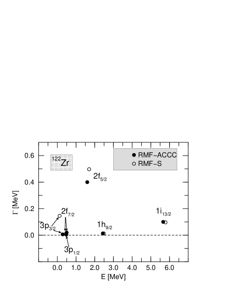
Figure 9: Energies and widths for the neutron states $\nu 3p_{3/2}$, $\nu 3p_{1/2}$, $\nu 2f_{7/2}$, $\nu 2f_{5/2}$, $\nu 1h_{9/2}$, and $\nu 1i_{13/2}$ in ¹²²Zr. Solid circles represent the results of the ACCC method, while open circles denote the results of the scattering method. Taken from Ref. [111].

The energies and widths for the neutron resonant states $\nu 3p_{3/2}$, $\nu 3p_{1/2}$, $\nu 2f_{7/2}$, $\nu 2f_{5/2}$, $\nu 1h_{9/2}$, and $\nu 1i_{13/2}$ in ¹²²Zr are shown in Fig. 9. The results of the ACCC and the scattering methods are in good agreement with each other for most of these states. From both methods, $\nu 2f_{5/2}$ and $\nu 1i_{13/2}$ have large widths, while $\nu 2f_{7/2}$ and $\nu 1h_{9/2}$ are very narrow. The width for $\nu 3p_{3/2}$ from the scattering method is slightly larger than that from the ACCC calculation. For the resonant state $\nu 3p_{1/2}$, neither the energy nor the width can be extracted from the scattering calculation. From a quantum mechanical point of view, these single-particle resonant states are quasi-stationary ones captured by centrifugal barriers. The decay width for a resonant state can be roughly explained by the penetration through the barrier. For those states with the same $l$, i.e., the same centrifugal barrier, the higher state has a larger width, e.g., for the two $f$ states $\nu 2f_{5/2}$ and $\nu 2f_{7/2}$. Although $\nu 1h_{9/2}$ is higher than $\nu 2f_{5/2}$, its width is smaller because of higher centrifugal barrier. A similar argument also holds for a much higher but narrow state $\nu 1i_{13/2}$.

3.2.2 BCS approximation with resonant states

The conventional BCS method is incapable of describing weakly bound nuclei due to the oscillating asymptotic behavior of single particle wave functions in the continuum [37]. Recently, many authors demonstrate that by picking up only those low-lying resonant states in the continuum, the BCS method can be successfully applied to weakly bound nuclei [97, 41, 115, 116, 117]. This is because the resonant states are well localized inside the nucleus and there is a large region outside the nucleus where the resonant wave functions have values close to zero before they start oscillating [97]. Therefore,the wave functions of the resonant states can be taken to be zero beyond a cutoff radius [97]. Meanwhile a realistic pairing potential, such as a zero-range $\delta$-force, prefer to pick up the resonant states, whose wave functions have a large overlap with those of bound states below the Fermi surface, rather than the continuum [115, 117]. In such a way, the HF+rBCS and RMF+rBCS results do not depend sensitively on the cutoff radius [97].

The BCS method can be easily extended to study the width effects of resonant states. The extended BCS equations for a general (finite range) pairing interaction including the contribution of the resonant continuum, referred as the resonant-BCS (rBCS) equations [97, 41], are :

$$\Delta_{i}=\sum_{j}V_{i\overline{i}j\overline{j}}u_{j}v_{j}+\sum_{\nu}V_{i\overline{i},\nu\epsilon_{\nu}\overline{\nu\epsilon_{\nu}}}\int_{I_{\nu}}g_{\nu}(\epsilon)u_{\nu}(\epsilon)v_{\nu}(\epsilon)d\epsilon~{},$$ (85)

$$\Delta_{\nu}\equiv\sum_{j}V_{\nu\epsilon_{\nu}\overline{\nu\epsilon_{\nu}},j\overline{j}}u_{j}v_{j}+\sum_{\nu^{\prime}}V_{\nu\epsilon_{\nu}\overline{\nu\epsilon_{\nu}},\nu^{\prime}\epsilon_{\nu^{\prime}}\overline{\nu^{\prime}\epsilon_{\nu^{\prime}}}}\int_{I_{\nu^{\prime}}}g_{\nu^{\prime}}(\epsilon^{\prime})u_{\nu^{\prime}}(\epsilon^{\prime})v_{\nu^{\prime}}(\epsilon^{\prime})d\epsilon^{\prime}~{},$$ (86)

$$N=\sum_{i}v_{i}^{2}+\sum_{\nu}\int_{I_{\nu}}g^{c}_{\nu}(\epsilon)v^{2}_{\nu}(\epsilon)d\epsilon~{}.$$ (87)

Here $\Delta_{i}$ are the gaps for the bound states and $\Delta_{\nu}$ are the averaged gaps for the resonant states. The quantity $\displaystyle g^{c}_{\nu}(\epsilon)=\frac{2j_{\nu}+1}{\pi}\frac{d\delta_{\nu}}{d\epsilon}$ is the total level density and $\delta_{\nu}$ is the phase shift of the state with the angular momentum $(l_{\nu}j_{\nu})$. The factor $g^{c}_{\nu}(\epsilon)$ can take into account the effect of the width and it is approximately a delta function for a very narrow resonance. The interaction matrix elements are calculated with the scattering wave functions at resonance energies and normalized inside a volume where the pairing interaction is active (see last paragraph).

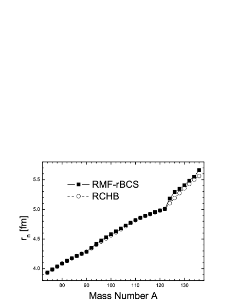
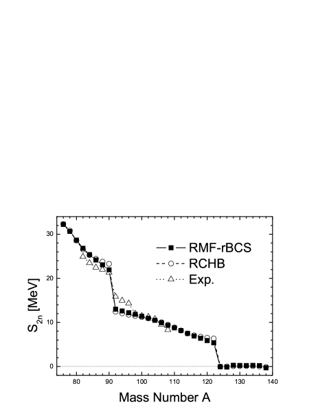
Figure 10: The rms neutron radii (left panel) and the two-neutron separation energies (right panel) of even Zr isotopes as a function of the mass number $A$. Taken from Ref. [41].

The BCS equations in the conventional RMF+BCS formalism can be easily substituted by these rBCS equations (85,86,87). To make this implementation, one can solve the RMF equations with the scattering-type boundary conditions or any other methods like the ACCC method described in the last subsection and find the energies, widths and wave functions for the resonant states. This approximation scheme, called the RMF+rBCS method, has been applied to study neutron-rich Zr isotopes [41]. It was demonstrated that the sudden increase of neutron radii close to the neutron drip line depends on a few resonant states close to the continuum threshold. Including these resonant states, the RMF-BCS calculations give practically the same neutron radii and neutron separation energies as the RCHB calculations (see Fig.10).

3.3 Relativistic continuum Hartree-Bogoliubov theory

3.3.1 Bogoliubov transformation and continuum spectra

The contribution of the resonant states can be self-consistently taken into account in the Hartree-Fock Bogoliubov (HFB) theory solved in the coordinate space [37]. The advantage of the general HFB theory is that the variation method based on quasi-particle transformation unifies the self-consistent description of nuclear orbitals and the BCS pairing theory into a single variation theory. In Fig. 11, schematic pictures for different bases in the HF, HFB and the canonical basis have been given. For a given many-body system, one can choose any $M$-dimension orthogonal and complete basis to diagonalize the Hamiltonian. That is shown in the first column of Fig. 11. If only HF approach are considered, the Hamiltonian is diagonal in the HF basis. We get a $M$-dimension basis, with a Fermi surface which divides the full open orbitals and full occupied orbitals. They are given in the second column. After the Bogoliubov transformation, we are working in the quasi-particle basis, which is enlarged into $2M$-dimension. The quasi-particle orbitals are reflection symmetric with respect to the Fermi surface, as shown in the third column. They must be transformed into the physical space — canonical basis [35, 42], in order to have a similar explanation as the HF space in the second column. For the Bogoliubov transformation involving the continuum, as the Fermi energy is negative for a bound nucleus, only those resonant states in the canonical basis with proper asymptotic behavior could be picked up. In the forth column, a schematic picture for the orbitals in the canonical basis is given, now the orbitals could be partially occupied, which is another essential difference between the HF basis and the canonical basis.

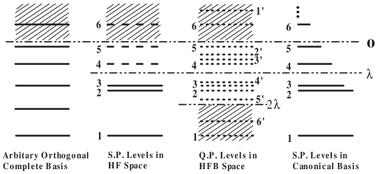
Figure 11: The schematic pictures of different basis. The first column is an arbitrary $M$-dimension orthogonal and complete basis to diagonalize the system Hamiltonian. The second column is the single particle levels in the HF space. The third column is quasi-particle levels in the quasi-particle HFB space which is enlarged into $2M$-dimension. The quasi-particle orbitals has a reflection symmetry with respect to the Fermi surface. The physical orbital in the canonical basis is given in the forth column.

3.3.2 The formalism for the RCHB theory

In the BCS approach, the gap equation takes into account only pairing between time-reversed continuum states. A more general pairing between continuum states at neighboring energies can be taken care of by a continuum Bogoliubov approach. The improvement to the BCS approximation is to introduce the concept of quasi-particle by the Bogoliubov transformation. Instead of introducing a mapping factor, the Bogoliubov transformation transforms the equation of motion into quasi-particle space. In the following we shall consider the transformation from the single particle basis to the quasi-particle basis. The single particle operators in coordinate space $a_{\mbox{r}}$,$a_{\mbox{r}}^{\dagger}$, are connected to the operators in the quasi-particle basis, $\beta_{i}$, $\beta_{i}^{\dagger}$, $i=1,M$, by the following transformation:

$$\left({\beta_{i}\atop\beta_{i}^{\dagger}}\right)=\int d^{3}\mbox{r}{\cal W}^{\dagger}\left({a_{\mbox{r}}\atop a_{\mbox{r}}^{\dagger}}\right)=\int d^{3}r\left(\begin{array}[]{cc}U_{i,\mbox{r}}^{*}&V_{i,\mbox{r}}^{*}\\ V_{i,\mbox{r}}&U_{i,\mbox{r}}\end{array}\right)\left({a_{\mbox{r}}\atop a_{\mbox{r}}^{\dagger}}\right),$$ (88)

where $i$ and r represents the row and column indices respectively. The basis of the quasi-particle states, $\psi_{U,i}({\mbox{\boldmath${\rm r}$}})$ and $\psi_{V,i}({\mbox{\boldmath${\rm r}$}})$, are defined via the single particle coordinate basis of $\delta$-function as:

$$\left(\psi_{U,i}({\mbox{\boldmath${\rm r}$}})\atop\psi_{V,i}({\mbox{\boldmath${\rm r}$}})\right)=\int d^{3}\mbox{r}^{\prime}\ \delta{(\mbox{r}-\mbox{r}^{\prime})}\ \left(U_{i,\mbox{r}^{\prime}}^{*}\atop V_{i,\mbox{r}^{\prime}}\right).$$ (89)

In spherical case, the Dirac spinor wave functions $\psi_{U,i}({\mbox{\boldmath${\rm r}$}})$ and $\psi_{V,i}({\mbox{\boldmath${\rm r}$}})$ are similar to Eq.(20) and satisfy the following normalization relation:

$$\int d^{3}r\cal W^{\dagger}\cal W=I.$$ (90)

The variation method based on quasi-particle transformation can unify the self-consistent description of nuclear orbitals, as given by the HF approach, and the BCS pairing theory into a single variation theory. As the equations of motion are self-consistently solved in the quasi-particle space, the convergence is guaranteed automatically. The unphysical continuum are excluded and the contribution from the resonance states with positive energies can be taken into account. From now on, the concept of continuum in Bogoliubov transformation is just the resonance states with positive energy as the unphysical continuum are excluded already.

Following the standard procedure of Bogoliubov transformation, a Dirac Hartree-Bogoliubov equation could be derived and the unified description of the mean field and pairing correlation in nuclei could be achieved. Using Green’s function techniques it has been shown in Refs. [95, 21] how one can derive a relativistic Hartree-Fock-Bogoliubov theory: after a full quantization of the system the mesonic degrees of freedom are eliminated and, in full analogy to the non-relativistic case, the higher order Green’s functions are factorized in the sense of Gorkov [118]. Finally, neglecting retardation effects and the Fock term, as it is mostly done in relativistic mean field theory, one ends up with RHB equations as the following:

$$\left(\begin{array}[]{cc}h-\lambda&\Delta\\ -\Delta^{*}&-h^{*}+\lambda\end{array}\right)\left({\psi_{U}\atop\psi_{V}}\right)~{}=~{}E~{}\left({\psi_{U}\atop\psi_{V}}\right),$$ (91)

where

$$h({\mbox{\boldmath${\rm r}$}},{\mbox{\boldmath${\rm r}$}}^{\prime})=\left[{{\mbox{\boldmath${\rm\alpha}$}}}\cdot{{\mbox{\boldmath${\rm p}$}}}+V({{\mbox{\boldmath${\rm r}$}}})+\beta(M+S({{\mbox{\boldmath${\rm r}$}}}))\right]$$ (92)

is the Dirac Hamiltonian and the Fock term has been neglected. The pairing potential is

$$\Delta_{kk^{\prime}}({\mbox{\boldmath${\rm r}$}},{\mbox{\boldmath${\rm r}$}}^{\prime}) = -\int d^{3}\mbox{r}_{1}\int d^{3}\mbox{r}_{1}^{\prime}\sum_{\tilde{k}\tilde{k}^{\prime}}V_{kk^{\prime},\tilde{k}\tilde{k}^{\prime}}({\mbox{\boldmath${\rm r}$}}{\mbox{\boldmath${\rm r}$}}^{\prime};{\mbox{\boldmath${\rm r}$}}_{1}{\mbox{\boldmath${\rm r}$}}_{1}^{\prime})\kappa_{\tilde{k}\tilde{k}^{\prime}}({\mbox{\boldmath${\rm r}$}}_{1},{\mbox{\boldmath${\rm r}$}}_{1}^{\prime}),$$ (93)

where $k$, $k^{\prime}$, $\tilde{k}$, or $\tilde{k}^{\prime}$ represent the other quantum numbers which together with the coordinate specify the single particle states. It is obtained from the pairing tensor,

$$\kappa_{kk^{\prime}}({\mbox{\boldmath${\rm r}$}},{\mbox{\boldmath${\rm r}$}}^{\prime})=\langle|a_{k,i}a_{k^{\prime},i^{\prime}}|\rangle=\sum_{E_{i}>0}\psi_{U}^{k,i}({\mbox{\boldmath${\rm r}$}})^{*}\psi_{V}^{k^{\prime},i}({\mbox{\boldmath${\rm r}$}}^{\prime}),$$ (94)

and one-meson exchange interaction $V_{kk^{\prime},\tilde{k}\tilde{k}^{\prime}}({\mbox{\boldmath${\rm r}$}}{\mbox{\boldmath${\rm r}$}}^{\prime};{\mbox{\boldmath${\rm r}$}}_{1}{\mbox{\boldmath${\rm r}$}}_{1}^{\prime})$ in the $pp$-channel. The nuclear density is given as

$$\rho({\mbox{\boldmath${\rm r}$}},{\mbox{\boldmath${\rm r}$}}^{\prime})=\sum_{k,E_{i}>0}\psi_{V}^{k,i}({\mbox{\boldmath${\rm r}$}})^{*}\psi_{V}^{k,i}({\mbox{\boldmath${\rm r}$}}^{\prime}).$$ (95)

In the RHB theory, the ground state $|\Psi\rangle$ of the even particle system is defined as the vacuum with respect to the quasi-particle: $\beta_{i}|\Psi\rangle=0$ for all $i$, i.e., $|\Psi\rangle=\prod_{i}\beta_{i}|-\rangle$, where $|-\rangle$ is the bare vacuum. For an odd particle system, the ground state can be correspondingly written as: $|\Psi\rangle_{j}=\beta_{j}^{\dagger}\prod_{i\neq j}\beta_{i}|-\rangle$, where $j$ is the level which is blocked. The exchange of the quasiparticle creation operator $\beta_{j}^{\dagger}$ with the corresponding annihilation operator $\beta_{j}$ means the replacement of the column $j$ in the $U$ and $V$ matrices by the corresponding column in the matrices $V^{*}$, $U^{*}$ [35].

As the one-meson exchange interactions are not able to reproduce even in a semi-quantitative way the proper pairing in the realistic nuclear many-body problem, the interaction $V$ in Eq. (93) is replaced by the phenomenological interaction which has been generally used in the pairing channel of the conventional HFB theory. As in Ref. [36] $V$ used for the pairing potential (93) is either the density-dependent two-body force of zero range:

$$V(\mbox{\boldmath$r$}_{1},\mbox{\boldmath$r$}_{2})=V_{0}\delta(\mbox{\boldmath$r$}_{1}-\mbox{\boldmath$r$}_{2})\frac{1}{4}\left[1-\mbox{\boldmath$\sigma$}_{1}\mbox{\boldmath$\sigma$}_{2}\right]\left(1-\frac{\rho(r)}{\rho_{0}}\right)$$ (96)

with the interaction strength $V_{0}$ and the nuclear matter density $\rho_{0}$ or Gogny-type finite range force:

$$V(\mbox{\boldmath$r$}_{1},\mbox{\boldmath$r$}_{2})~{}=~{}\sum_{i=1,2}e^{((\mbox{\boldmath$r$}_{1}-\mbox{\boldmath$r$}_{2})/\mu_{i})^{2}}(W_{i}+B_{i}P^{\sigma}-H_{i}P^{\tau}-M_{i}P^{\sigma}P^{\tau})$$ (97)

with the parameter $\mu_{i}$, $W_{i}$, $B_{i}$, $H_{i}$ and $M_{i}$ ($i=1,2$) as the finite range part of the Gogny force D1S [119].

The RHB equations can be solved in different bases as well. In many applications an expansion of the wave functions in an appropriate harmonic-oscillator basis of spherical or axial symmetry provides a satisfactory level of accuracy. For example, in Ref. [120] the RHB equations were solved by expanding the nucleon spinors $U_{k}(r)$ and $V_{k}(r)$ and the meson fields in a basis of spherical harmonic oscillators. However, for nuclei near the drip lines the expansion in the localized oscillator basis presents only a poor approximation for the continuum states. Oscillator expansions produce densities which decrease too steeply in the asymptotic region at large distance from the center of the nucleus. The calculated rms radii cannot reproduce the experimental values, especially for halo nuclei. The transformed harmonic oscillator (THO) basis has also been employed in the solution of the RHB equations in configurational space [64]. Solving the RHB equations in Woods-Saxon basis is another alternative.

In order to describe the coupling between bound and continuum states more exactly, the RHB equations and the equations for the meson fields should be solved in coordinate space [42, 36, 121] and one arrives at the RCHB theory. When spherical symmetry is imposed, the wave function can be conveniently written as

$$\psi^{i}_{U}=\left({\displaystyle{i\frac{G_{U}^{i\kappa}(r)}{r}}\atop{\displaystyle\frac{F_{U}^{i\kappa}(r)}{r}({\mbox{\boldmath${\rm\sigma}$}}\cdot\hat{{\mbox{\boldmath${\rm r}$}}})}}\right){Y^{l}_{jm}(\theta,\phi)}\chi_{t}(t),~{}~{}~{}\psi^{i}_{V}=\left({\displaystyle{i\frac{G_{V}^{i\kappa}(r)}{r}}\atop{\displaystyle\frac{F_{V}^{i\kappa}(r)}{r}({\mbox{\boldmath${\rm\sigma}$}}\cdot\hat{{\mbox{\boldmath${\rm r}$}}})}}\right){Y^{l}_{jm}(\theta,\phi)}\chi_{t}(t).$$ (98)

The above equation (91) only depends on radial coordinates and can be derived as the following integro-differential equations:

$$\left\{\begin{array}[]{lll}\displaystyle\frac{dG_{U}(r)}{dr}+\frac{\kappa}{r}G_{U}(r)-(E+\lambda-V(r)+S(r))F_{U}(r)+r\int r^{\prime}dr^{\prime}\Delta(r,r^{\prime})F_{V}(r^{\prime})&=&0,\\ \displaystyle\frac{dF_{U}(r)}{dr}-\frac{\kappa}{r}F_{U}(r)+(E+\lambda-V(r)-S(r))G_{U}(r)+r\int r^{\prime}dr^{\prime}\Delta(r,r^{\prime})G_{V}(r^{\prime})&=&0,\\ \displaystyle\frac{dG_{V}(r)}{dr}+\frac{\kappa}{r}G_{V}(r)+(E-\lambda+V(r)-S(r))F_{V}(r)+r\int r^{\prime}dr^{\prime}\Delta(r,r^{\prime})F_{U}(r^{\prime})&=&0,\\ \displaystyle\frac{dF_{V}(r)}{dr}-\frac{\kappa}{r}F_{V}(r)-(E-\lambda+V(r)+S(r))G_{V}(r)+r\int r^{\prime}dr^{\prime}\Delta(r,r^{\prime})G_{U}(r^{\prime})&=&0,\\ \end{array}\right.$$ (103)

where the nucleon mass has been included in the scalar potential $S(r)$. Instead of solving Eqs. (21) and (23) self-consistently for the RMF case, now one has to solve Eqs. (103) and (23) self-consistently for the RCHB case. The densities are calculated as

$$\left\{\begin{array}[]{lll}4\pi r^{2}\rho_{s}(r)&=&\sum_{i}(|G^{i}_{V}(r)|^{2}-|F^{i}_{V}(r)|^{2}),\\ 4\pi r^{2}\rho_{v}(r)&=&\sum_{i}(|G^{i}_{V}(r)|^{2}+|F^{i}_{V}(r)|^{2}),\\ 4\pi r^{2}\rho_{3}(r)&=&\sum_{i}\tau_{3}(|G^{i}_{V}(r)|^{2}+|F^{i}_{V}(r)|^{2}),\\ 4\pi r^{2}\rho_{c}(r)&=&\sum_{i}\frac{1}{2}(1-\tau_{3})(|G^{i}_{V}(r)|^{2}+|F^{i}_{V}(r)|^{2}),\\ \end{array}\right.$$ (108)

where the summations are over all quasi particle states. From the densities given above, one can calculate the rms radii and charge radius of the nucleus. The total binding energy is calculated as

$$E = E_{\rm nucleon}+E_{\sigma}+E_{\omega}+E_{\rho}+E_{c}+E_{\rm CM},$$ (109)

where except for $E_{\rm nucleon}$, the other terms are the same as those in the spherical RH theory. The energy of nucleons $E_{\rm nucleon}$ is calculated as

$$E_{\rm nucleon}=\sum_{i}\int dr(\lambda-E^{i})\left[|G^{i}_{V}(r)|^{2}+|F^{i}_{V}(r)|^{2}\right]-2E_{\rm pair},$$ (110)

and $E_{\rm pair}=-\frac{1}{2}{\rm Tr}\Delta\kappa$. For the details of the transformation from the quasi particle space to the canonical basis, the reader is referred to Ref. [42].

To solve RCHB equations (103), one has to discretize the RCHB continuum. The discretization can be done by solving the RCHB equation in a spherical box of radius $R$, i.e., by imposing the boundary conditions

$$\psi_{U}(E,|{\mbox{\boldmath${\rm r}$}}|=R,s)=\psi_{V}(E,|{\mbox{\boldmath${\rm r}$}}|=R,s)=0.$$ (111)

By increasing $R$, one can make the RCHB spectrum dense and better approximate the continuum, while increasing $E_{max}$ allows one to take into account coupling to highly excited quasi-particle state. Both $R$ and $E_{max}$ must be reasonably taken in such a way that the final results do not depend on the chosen $R$ and $E_{max}$. Only those solutions with $E>0$ are necessary due to the special symmetry of RCHB equation [42]. If $E$ is the solution of Eq. (91), $-E$ must be another solution, but they are not independent. Both solutions are connected as following:

$$\psi_{U}^{i}(-E,{\mbox{\boldmath${\rm r}$}})=\psi_{V}^{i}(E,{\mbox{\boldmath${\rm r}$}}),~{}~{}\psi_{V}^{i}(-E,{\mbox{\boldmath${\rm r}$}})=-\psi_{U}^{i}(E,{\mbox{\boldmath${\rm r}$}}).$$ (112)

So one can concentrate only on the solution with either positive energies or negative energies.

Equations (103), in the case of $\delta$-force  Eq.(96), is reduced to ordinary coupled differential equations and can be solved with shooting method combined with Runge-Kutta algorithms, which is so far the most elegant method for coupled differential equations in coordinate representation. For each fixed value of the energy $E$ the RCHB equations (103) are solved in the following steps:

1. Discretizing the whole space $[0,\infty]$;

2. Choosing a value for the energy $E$ in Eq. (103) with $E\geq 0$ for the given spin-parity channel;

3. Finding the proper boundary condition for $\psi(0)$, where $\psi$ represents $G_{V}$,$F_{V}$,$G_{U}$,$F_{U}$ and integrated Eq. (103) outward from $r=0$ to proper matching point $r=R_{match}$ by Runge-Kutta algorithms;

4. Finding the proper boundary condition for $\psi(\infty)$ and integrated Eq. (103) from $r=\infty$ inward to proper matching point $r=R_{match}$ by Runge-Kutta algorithms;

5. Requiring the $\psi(r)$ derived from the former two steps to be the same at $r=R_{match}$ will lead to the correct energy $E$;

6. Repeating the process till all the energies in the given spin-parity channel lying in $[0,E_{cut}]$ have been found.

Equations (103) for Gogny forces (97) are a set of four coupled integro-differential equations. They are discretized in the space and solved by the finite element method as the following:

1. Discretizing the whole space $[0,\infty]$ with $N+1$ points at $r_{1}=0,r_{2}=\rho,...,r_{N+1}=N\times\rho$, where $\rho=R/N$.

2. Assuming $\psi(r)$ at $r_{1}=0,r_{2}=\rho,...,r_{N+1}=N\times\rho$ are known, if $\rho=R/N$ is small enough, $\psi(r)$ in the element $(i-1)\times\rho\leq r\leq i\times\rho$ could be written as a simple linear combination of $\psi(r_{i})$ and $\psi(r_{i+1})$;

3. Requiring Eqs. (103) is valid in the element $(i-1)\times\rho\leq r\leq i\times\rho$, which could be easily integrated analytically and lead to a simple relation for $E$, $\psi(r_{i})$ and $\psi(r_{i+1})$;

4. Repeating the process for all the $N$ element, one then is lead to a $4\times(N+1)$ linear algebra equations for $E$, $G_{V}$,$F_{V}$,$G_{U}$,$F_{U}$ for $r=r_{1},r_{2},...,r_{N+1}$, which is nothing but a generalized eigenvalue problem;

5. Diagonalizing this generalized eigenvalue problem one can get all the energies and their wave function discretized at $r=r_{1},r_{2},...,r_{N+1}$.

Normally, equations (103) and (23) are solved in a self-consistent way by the shooting method or finite element methods with a step size of $0.1$ fm using proper boundary conditions in a spherical box of radius $R\leq 20$ fm. The Fermi-surface $\lambda$ is determined self-consistently by the particle number [42]. The results do not depend on the box size for $R>15$ fm [43]. For $\delta$-force (96), the number of continuum levels is limited by a cut-off energy, which must be larger than the depth of the potentials.

3.3.3 Pairing correlation: finite range vs. zero range

In the vicinity of the drip line, as the contribution from the continuum is switched on, it is very challenging to have the proper single particle levels and treat the coupling of the continuum without any ambiguity. Therefore, a proper interaction for the coupling between the bound state and the continuum is also essential. In principle, the effective nucleon-nucleon interaction should be obtained by means of Bruckner renormalization which gives the correct interaction after modifying the free interaction for the effect of the nuclear medium. In practice, however, the effective interactions are approximated by some phenomenological forces, such as Skyrme-type $\delta$-force or finite range Gogny force. Delta force is relatively simple for numerical calculation and has a realistic density-dependent behavior, but it allows a coupling to the very highly excited states. Normally an energy cutoff has to be introduced and the interaction strength has to be properly justified. The Gogny force has a better treatment for the coupling to the highly excited states, but it involves more sophisticated numerical techniques.

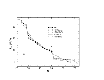
Figure 12: Left: Two-neutron separation energies $S_{2n}$ of even Ni isotopes as a function of $N$, including the experimental data (solid points), RCHB with $\delta$-force (open circles), RCHB with Gogny force (triangles) ,HFB with SkP interaction (stars) and HFB with SIII interaction (pluses); Right: The neutron pairing energies for RCHB with Gogny force (triangles) and $\delta$-force (open circles). The open circles connected by dashed line or solid line are respectively the pairing energies for RCHB with $\delta$-force by fitting that of RCHB with Gogny force at ⁵²Ni or ⁹⁰Ni. Taken from [122].

The Skyrme- and Gogny-type pairing forces have been discussed before within the conventional HFB formalism, but the HFB equations for Gogny force are solved on a harmonic basis, which is valid only for stable nuclei. In Ref. [122], the proper form of the pairing interaction near the drip line is discussed in the framework of the RCHB theory. The chain of even-even nickel isotopes ranging from the proton drip line to the neutron drip line are taken as examples. The pairing correlations are taken into account by either a density-dependent force of zero range or the finite range Gogny force. Through the comparisons of the two neutron separation energies $S_{2n}$, the neutron, proton, and matter rms radii, excellent agreements have been found between the calculations with both interactions and the empirical values. In Fig. 12, for example, the two neutron separation energies $S_{2n}$ of even Ni isotopes are shown as a function of the neutron number $N$ from the proton drip line to the neutron drip line, including the experimental data (solid points), RCHB with $\delta$-force (open circles), RCHB with Gogny force (triangles), HFB with SkP interaction [38] (stars) and SIII interaction [123] (pluses). The RCHB results with $\delta$-force and Gogny force are almost identical. They show a strong kink at $N$=28 and a less one at $N$=50. The drip line nucleus is predicated at ¹⁰⁰Ni in both calculations. The empirical data is known only up to $N$=50. Comparing with the available empirical data, the general trend and gradual decline of $S_{2n}$ have been well reproduced.

The neutron pairing energies $-\frac{1}{2}\mbox{Tr}\Delta\kappa$ for the calculation of RCHB with Gogny force are given in Fig. 12 as triangles. The pairing energies demonstrate the shell structure revealed by the $S_{2n}$ in Fig. 12. They vanish at the closure shell and have a maximum values in the middle of two neighboring closure shells. A tendency of the enhancement of pairing energies appears for the neutron-rich nuclei. The pairing energies for RCHB with $\delta$-force are given by open circles. The circles connected by the solid line and dashed line are calculations with $V_{0}=742$ MeV$\times$fm^-3 (by fitting the pairing energy of the Gogny force at ⁹⁰Ni) and $715$ MeV$\times$fm^-3 (by fitting at ⁵²Ni), respectively. The variation behavior of the pairing energies with $N$ is quite similar, although $V_{0}$ fitted at ⁹⁰Ni gives 2 MeV more for stable nuclei and $V_{0}$ fitted at ⁵²Ni gives 4 MeV less for neutron rich nuclei. But these differences have little influence on the two-neutron separation energies and the rms radii, as one observes in Fig. 12, for example. This clearly demonstrated the reliability of the result against the pairing strength.

Figure 13: The occupation probabilities in the canonical basis for ⁹⁰Ni as a function of the single particle energy around the threshold, for RCHB with $\delta$-force (dashed line) and Gogny force (solid points). Taken from [122].

Another interesting feature of the exotic nuclei is the contribution from the continuum. Definitely it is very interesting to see how different the contribution from the continuum is for the calculations with Gogny force and $\delta$-force. In Fig. 13 the occupation probabilities of ⁹⁰Ni in the canonical basis is shown [35] for the neutron levels near the Fermi surface, i.e. in the interval $-10\leq E_{s.p.}\leq 10$ MeV. The occupation probabilities for RCHB $\delta$-force are represented by the dashed line and RCHB with Gogny force by the solid points. For $V_{0}=715$ MeV$\times$fm^-3 or $V_{0}=742$ MeV$\times$fm^-3, the occupation probabilities are the same. Even the difference from the Gogny and the $\delta$-force is too small to have any influence on the physical observables like $S_{2n}$ and rms radii.

It has been shown that after proper renormalization (e.g., fixing the corresponding pairing energies), physical observables such as $S_{2n}$ and rms radii remain the same, even within a reasonable region of the interaction strength [122].

4 Exotic nuclei

The study of exotic nuclei has attracted world wide attention due to their large $N/Z$ ratios (isospin) and interesting properties such as halo and skin. It is also important for other fields including astrophysics, e.g., the properties of exotic nuclei are essential to understand the nucleosynthesis in the r process. Since the first case of halo in an exotic nucleus ¹¹Li was observed with RIB in 1985 [13], more and more exotic nuclei have been investigated with various modern experimental methods to understand this attractive phenomenon better [6, 7, 8, 11, 12]. For nuclei far from the $\beta$-stability valley and with small nucleon separation energy, the valence nucleons in exotic nuclei extend over quite a wide space to form low density nuclear matter. Furthermore, the Fermi surface for exotic nuclei is usually very close to the continuum threshold. The valence nucleons could be easily scattered to the continuum states due to the pairing correlation. Thus, theories which can properly handle the pairing and continuum states are needed to describe the properties of exotic nuclei. One of such theories is the RCHB theory [36, 42] introduced in the previous section. In this section, the RCHB theory will be applied to study the properties of exotic nuclei, e.g., the binding energies, particle separation energies, the radii and cross sections, the single particle levels, shell structure, the restoration of the pseudo-spin symmetry, the halo and giant halo, and halos in hyper nuclei, etc.

4.1 Binding and separation energies

The self-consistent microscopic RCHB theory has been used to study the ground state properties systematically such as binding energy, separation energy, radius, density distribution, single particle spectrum and shell structure etc. for a large number of isotope chains from the proton drip line to the neutron drip line throughout the periodic table including Li, C, N, O, F, Na, Ca, Ni, Zr, Sn and Pb [36, 43, 42, 45, 122, 124, 32, 46, 44, 125, 126, 47]. In this subsection, we will briefly present the description of the binding energies and separation energies for some typical spherical nuclei in RCHB theory.

Ground state properties of all the even-even O, Ca, Ni, Zr, Sn, Pb isotopes ranging from the proton drip line to the neutron drip line were investigated with the RCHB theory [126]. The binding energy $E_{b}$ calculated from the RCHB theory for these isotope chains and the corresponding data available [89] are compared. Generally speaking, the calculations reproduce the available data of binding energy quite well. The errors are usually within 3-4 MeV which is less than $1\%$ of the experimental values. Since the deformation effects are not included in the RCHB calculations yet, for some nuclei with large deformation, larger discrepancies ($\Delta E_{b}\sim 10$ MeV) of binding energy from experimental values are found, e.g., in some Zr isotopes.

Figure 14: The two neutron separation energies $S_{2n}$ for the proton magic isotopes plotted as a function of the neutron number in RCHB with NLSH. The experimental values are denoted by the solid symbols and the calculated ones by the open symbols. Taken from Ref. [126].

In Table 5, the binding energies for Pb isotopes calculated with different effective interactions PK1, PK1R, PKDD, TM1, NL3, TW99 and DD-ME1 are given in comparison with the experimental values [51]. Many effective interactions, particularly PK1, PK1R and PKDD provide good descriptions of the available data. All the effective interactions overestimate the binding energy in the beginning of the isotopic chain. However, from ¹⁹⁰Pb to ²¹⁰Pb, the effective interactions PK1, PK1R and PKDD give better descriptions than all the others. There exist however systematic deviations out of the neutron magic numbers, e.g., in ²¹⁴Pb. For the effective interactions TM1, NL3, TW99 and DD-ME1, the deviations in ²¹⁴Pb are smaller but fairly large in ²⁰⁸Pb.

The one or two nucleon separation energies $S_{p(n)}$ or $S_{2p(2n)}$ are quite sensitive quantities to test a microscopic theory. In Fig. 14 both the theoretical and the available experimental $S_{2n}$ are presented as a function of neutron number $N$ for the O, Ca, Ni, Zr, Sn, Pb isotope chains, respectively. The good coincidence between experiment and calculation is clearly seen. Seen along the $S_{2n}$ versus $N$ curve in Fig. 14, strong kinks can be clearly seen at $N=8$, $N=20,28,40$, $N=28,50$, $N=50,82$ and $N=126$ for O, Ca, Ni, Zr, Sn, Pb isotope chains, respectively. All these numbers correspond to the neutron magic numbers, which come from the large gaps of single particle energy levels.

Table 5: Total binding energies of Pb isotopes (in MeV) calculated with the nonlinear self-coupling effective interactions PK1, PK1R and the density-dependent meson-nucleon coupling effective interaction PKDD [51], in comparison with the experimental values [89] and the results of TM1, NL3, TW99 and DD-ME1.

$A$	Exp.	PK1	PK1R	PKDD	NL3	TM1	TW99	DD-ME1
182	1411.650	1416.431	1416.619	1416.309	1415.184	1420.872	1417.202	1415.216
184	1431.960	1435.548	1435.706	1435.478	1434.569	1439.768	1436.761	1434.569
186	1451.700	1454.258	1454.382	1454.192	1453.511	1458.222	1455.879	1453.306
188	1470.900	1472.586	1472.673	1472.504	1472.056	1476.272	1474.640	1471.639
190	1489.720	1490.555	1490.603	1490.468	1490.247	1493.958	1493.109	1489.657
192	1508.120	1508.197	1508.201	1508.116	1508.130	1511.317	1511.329	1507.411
194	1525.930	1525.536	1525.494	1525.474	1525.733	1528.378	1529.309	1524.937
196	1543.250	1542.592	1542.502	1542.545	1543.085	1545.163	1547.012	1542.262
198	1560.070	1559.378	1559.236	1559.329	1560.199	1561.685	1564.338	1559.403
200	1576.365	1575.893	1575.697	1575.831	1577.076	1577.942	1581.344	1576.365
202	1592.202	1592.095	1591.843	1592.022	1593.679	1593.905	1598.084	1593.133
204	1607.520	1607.851	1607.545	1607.770	1609.906	1609.477	1614.197	1609.676
206	1622.340	1623.126	1622.765	1623.167	1625.725	1624.530	1630.122	1625.966
208	1636.446	1637.443	1637.024	1637.387	1640.584	1638.777	1644.790	1641.415
210	1645.568	1644.844	1644.345	1643.643	1647.969	1647.245	1650.888	1648.312
212	1654.524	1652.155	1651.573	1649.873	1655.289	1655.549	1657.020	1655.174
214	1663.298	1659.382	1658.718	1656.084	1662.551	1663.706	1663.196	1662.011
$\sigma$		0.00033	0.00036	0.00042	0.00031	0.00068	0.00078	0.00033

For the proton magic even mass nuclei studied in Ref. [126], the neutron drip line nuclei are predicted as ²⁸O, ⁷²Ca, ⁹⁸Ni, ¹³⁶Zr, ¹⁷⁴Sn, and ²⁶⁶Pb, respectively. In Refs. [127, 128], the last bound nucleus in neutron rich Ca isotopes is predicted as ⁷⁰Ca with the HFB and Skyrme HF methods, respectively. The reason for that ⁷²Ca is bound is caused by the halo effect, which also results in the disappearance of the normal $N=50$ magic number in the RCHB calculation as shown in Fig. 14 where no kink appears at $N=50$ for Ca isotopes. In stable nuclei, the $N=50$ magic number is given by the big energy gap between the $1g_{9/2}$ and $3s,~{}2d$ levels. However in the vicinity of the drip line region of Ca isotopes, the single particle energy of $3s_{1/2}$ would decrease with the halo effect and its zero centrifugal potential barrier, the large gap between $1g_{9/2}$ and $3s_{1/2}$ disappears. Therefore, the nucleus ⁷⁰Ca is no more a doubly magic nucleus and ⁷²Ca is bound. This disappearance of the $N=50$ magic number at the neutron drip line is due to the halo property. This is different from the disappearance of the $N=20$ magic number which is due to deformation. Recently a new magic number $N=16$ has been discovered in neutron drip line light-nuclei region which is also considered as owing to the halo effect [14]. It can be expected that near drip line, more traditional magic numbers would disappear and new magic numbers would be found with the same mechanism.

Figure 15: The one neutron separation energies $S_{\rm n}$ for the nuclei ^11-22C,^13-24N,^15-26O and ^17-25F by RCHB theory(open circles) and their experimental counterparts (solid circles). Taken from Ref. [46].

Systematic RCHB calculations with NLSH have been carried out for the C, N, O and F isotopes [46]. The one neutron separation energies $S_{\rm n}$ predicted by RCHB and the data [89] for the nuclei ^11-22C, ^13-24N, ^15-26O and ^17-25F are shown in Fig. 15 as open and solid circles respectively. For carbon isotopes, the theoretical one neutron separation energies for ^11-18,20,22C are in agreement with the data. The calculated $S_{\rm n}$ is less than 0 ($-$0.003 MeV) for the odd-$A$ nucleus ¹⁹C which is bound in experiment. While for the experimentally unbound nucleus ²¹C, the predicted value of $S_{\rm n}$ is positive. From the neutron-deficient side to the neutron drip line, excellent agreement has been achieved for the nitrogen isotopes. As almost all relativistic mean field approaches do, the RCHB calculations overestimate binding for ^25,26O which are unstable in experiment. For fluorine isotopes, the $S_{\rm n}$ in ^17,26-29F are overestimated in contrast with the underestimated one in ¹⁸F. The last bound neutron-rich nucleus is predicted as ³⁰F. In general, the RCHB theory reproduces the $S_{\rm n}$ data well considering that this is a microscopic and almost parameter free model. As discussed above, there are some discrepancies between the calculations and the empirical values for some of the studied isotopes. This may be due to deformation effects, which has been neglected in Ref. [46].

4.2 Radius, nuclear density distribution, and cross section

4.2.1 Nuclear root mean square radii

The nuclear radii are important basic physical quantities to describe atomic nuclei. The calculated neutron, proton, matter, and charge radii for all even Ca isotopes against mass number $A$ are plotted in Fig. 16. For nuclear charge radii $r_{c}$, the well-known parabolic behavior along ^40-48Ca is not reproduced in RCHB calculation. It is mainly due to the improper spherical supposition to the real deformed ^42,44,46Ca nuclei. It can be clearly seen that the radii $r_{p}$, $r_{n}$, $r_{m}$ and $r_{c}$ all increase with the mass number $A$. The mass radii $r_{m}$ as well as $r_{n}$ increase much faster than $r_{p}$ and $r_{c}$. In addition to the normal increase of $r_{n}$ and $r_{m}$ with $A$, a slightly up-bend tendency occurs in the neutron drip line region from $A=62$ up to $A=72$.

Figure 16: The rms radii for the proton, neutron, charge and matter distributions are plotted as a function of the neutron number for the Ca isotope. The available experimental values are denoted by solid symbols. Taken from Ref. [126].

For light nuclei, the RCHB calculations predict a slight increase of proton or charge radii when the proton drip line is approached [46]. The neutron and proton rms radii predicted by RCHB for the nuclei ^10-22C, ^12-24N,^14-26O and ^16-25F are given in Fig. 17. The neutron radii for nuclei in each isotope chain increase steadily. While the corresponding proton radii remains almost constant for nuclei in each isotope chain except for proton rich ones. The increase of proton radii with neutron number decreasing in the proton rich side in each isotope chain is responsible for the slightly increase in the charge changing cross section of these nuclei on the target ¹²C as discussed in Section 4.2.4.

Figure 17: The neutron and proton rms radii predicted by RCHB for the nuclei ^10-22C, ^12-24N,^14-26O and ^16-25F. Taken from Ref. [46].

In Fig. 18 the neutron radii $r_{n}$ from the RCHB calculation for the even-even nuclei of the O, Ca, Ni, Zr, Sn and Pb isotope chains are ploted. The predicted $r_{n}$ curve using the simple empirical equation $r_{n}=r_{0}\cdot N^{1/3}$ with $r_{0}=1.139$ normalizing to ²⁰⁸Pb is also represented in the figure. The simple formula for $r_{n}$ agrees with the calculated neutron radii except for two anomalies. One anomaly appears in the Ca chain above $N=40$, and the other in Zr chain above $N=82$. The increase of exotic Ni and Sn nuclei is not as rapid as that in Ca and Zr chains. The regions of the abnormal increases of the neutron radii are just the same as those for $S_{2n}$. Both behaviors are connected with the formation of giant halo (see Section 4.4 for details).

Figure 18: The rms neutron radii for the proton magic even mass nuclei plotted as a function of the neutron number. The solid curve corresponds to the radii calculated with the $N^{1/3}$ formula.

It is interesting to investigate the neutron number dependence of the proton radii (or charge radii) and the neutron radii for these proton-magic isotope chains. In Fig. 19, the rms charge radii $r_{c}$ obtained from the RCHB theory (open symbols) and the data available (solid symbols) for the even-even Ca, Ni, Zr, Sn and Pb isotopes are shown. The RCHB calculations reproduce the data very well (within 1.5$\%$). For a given isotopic chain, an approximate linear $N$ dependence of the calculated rms charge radii $r_{c}$ is clearly seen. However, the variation of $r_{c}$ for a given isotopic chain deviates from the general accepted simple $A^{1/3}$ law (denoted by dashed lines in Fig. 19), which shows a strong isospin dependence of nuclear charge radii for nuclei with extreme $N/Z$ ratio. Recently, these charge radii as well as the large amount of experimental data are investigated. A formula with the $Z^{1/3}$ dependence and isospin dependence is proposed which describes well the charge radii all over the nuclear isotope chart, see subsection 4.2.3. [129].

4.2.2 Neutron skin thickness

The measurement of nucleon density distributions provides basic and important information in nuclear structure. The proton distribution of stable nuclei can be determined accurately by elastic electron or muon scattering. However, there is not comparable measurement of the neutron density distribution up to now. Although it is difficult to obtain the neutron density distribution, the difference in radii of the neutron and proton density distributions can be more easily determined [130]. Theoretically, the neutron skin thickness, $r_{\mathrm{n}}-r_{\mathrm{p}}$ could place important constraints on effective interactions used in nuclear models [131, 132, 133].

Many investigations have been done aiming at the description of the neutron skin thickness in the framework of the RMF model. With the pairing correlation treated by a constant BCS approach, the neutron rms radii of some closed and open shell nuclei are investigated with the spherical RMF model [134]. It has been demonstrated that with an increase in isospin of nuclei, the neutron rms radii in the relativistic mean-field approach with the parameter sets NL1 and NL2 are larger than both the empirical data and the predictions of the Skyrme mean field [135]. This overestimation of the neutron skin thickness remains true for the effective interaction NL3, although the relativistic Hartree-Bogoliubov model with NL3+D1S give a good result of the neutron-skin thickness along the Sn isotopic chain compared to the available data [136, 137].

The overestimation of the neutron skin thickness is attributed to a poor description of the isovector channel of the nonlinear effective interaction in Ref. [62] where the RHB model is extended to include density-dependent meson-nucleon couplings. A density-dependent effective interaction DD-ME1 is proposed in which the improved isovector properties result in a better description of charge radii, and especially the calculated values of neutron thickness are in much better agreement with experimental data. As what is shown in Fig. 19, the difference between the values calculated with NL3 and DD-ME1 increases with the number of neutrons to about 0.1 fm at $N$ = 82, but then it remains practically constant for $N>$ 82. While both interactions reproduce the isotopic trend of the experimental data, NL3 obviously overestimates the neutron skin. The values calculated with DD-ME1, on the other hand, are in excellent agreement with the experimental data. This result presents a strong indication that the isovector channel of the effective interaction DD-ME1 is correctly parametrized.

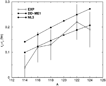
Figure 19: DD-ME1 and NL3 predictions for the neutron skin thickness of Sn isotopes, compared with experimental data. Taken from Ref. [62].

In Ref. [133], the sensitivity of the neutron skin thickness $S=r_{\mathrm{n}}-r_{\mathrm{p}}$ in ²⁰⁸Pb to the addition of nucleon-$\sigma$-$\rho$ coupling corrections to a selection (PK1, NL3, S271, and Z271) of interactions in RMF model was investigated. With the higher order nucleon-$\sigma$-$\rho$ coupling, the PK1 and NL3 effective interactions lead to a minimum value of the neutron skin thickness $S$ = 0.16 fm and the S271 and Z271 effective interactions yield even smaller values of $S$ = 0.11 fm. The addition of these higher order correction terms to the conventional RMF models can be associated with some kind of multimeson exchange processes occurring in the inner (higher density) region of nuclei. In the inner region of a heavy nucleus such as ²⁰⁸Pb, one could imagine that multimeson exchange processes introduced through nucleon-$\sigma$-$\rho$ coupling corrections could play an important role in modifying the short-range behavior of the nucleon-nucleon interaction, by softening the density dependence of the symmetry energy at high density (the inner part of nuclei) and thus leading to smaller values of neutron skin thickness $S$ compared to previous effective interactions.

4.2.3 Nuclear charge radii: isospin dependence and the $Z^{1/3}$ law

Among all the size quantities describing nucleus, nuclear charge radius has been measured with very high precision by various techniques and methods experimentally. With its accuracy, the study of the nuclear charge radii is very important to understand not only the proton distribution inside the nucleus but also the exotic phenomena such as halo and skin observed in exotic nuclei. Particularly if one can get a simple and reliable formula for nuclear charge radii, it will be very useful to extract the decoupling of proton and neutron in the exotic nuclei and provide information for the effective nucleon-nucleon interaction widely used in all the nuclear models. The available charge radii data for $A\geq 40$ were examined and its global behavior was studied in Ref. [129]. Instead of the widely accepted $A^{1/3}$ law, a new $Z^{1/3}$ formula with isospin effect has been proposed.

Based on the consideration of the nuclear saturation property, nuclear charge radius $R_{c}$ is usually described by the $A^{1/3}$ law [16, 35]

$$R_{c}=r_{A}A^{1/3},$$ (113)

where $A$ is the mass number and $R_{c}=\sqrt{5/3}~{}r_{c}$, with $r_{c}$ the rms charge radius. For very light nuclei, because of their small $A$ and large fluctuation in charge distribution due to the shell effect with short period, it seems that the charge distribution radius as a bulk property has little meaning. A detailed analysis of charge radii data for $A\geq 40$ shows that $r_{A}$ is by no means a constant, but systematically decreases with $A$; i.e., $r_{A}\approx 1.31$ fm for light nuclei $(A\sim 40)$ and $r_{A}\approx 1.20$ fm for very heavy nuclei (see upper left panel in Fig.  20). This fact implies that some physics is missing in Eq. (113).

Definite evidences of the violation of $A^{1/3}$ law have been found in the measurements of isotope shift in rms charge radii [138, 139, 140]. In particular, $\delta\langle r^{2}\rangle_{A+2,A}$ values (associated with an addition of two neutrons) are often found to be considerably smaller compared to what is expected from the $A^{1/3}$ law ($\delta\langle r^{2}\rangle_{A+2,A}=\frac{4}{3A}\langle r^{2}\rangle_{A}$). A typical example is that the observed charge radii of the calcium isotopes ^40-50Ca remain almost the same (except a very little change induced by deformation or shell effect), though the mass number $A$ has changed significantly. In contrast, there is also evidence that the observed $\delta\langle r^{2}\rangle_{A+2,A}$ values (associated with the addition of two protons) are often greater than what is expected from the $A^{1/3}$ law (e.g., $\delta\langle r^{2}\rangle$ for ⁴⁶Ti$-^{44}$Ca, ⁵⁰Ti$-^{48}$Ca, etc.).

Along the $\beta$-stability line, the ratio $Z/A$ gradually decreases with $A$, i.e., for light nuclei $Z/A\approx 1/2$, and for the heaviest $\beta$-stable nucleus ${}^{238}_{\ 92}$U, $(Z/A)^{1/3}\approx 0.7285$. It turns out that $(1/2)^{1/3}/0.7285\approx 1.09$, which is very close to the $r_{A}$ ratio $1.30/1.20$ shown in the upper left panel of Fig. 20. A naive point of view is that the charge radius of a nucleus may be more directly related to its charge number $Z$, rather than its mass number $A$. Therefore, compared to the $A^{1/3}$ law, a $Z^{1/3}$ dependence for nuclear charge radii may be more reasonable,

$$R_{c}=r_{Z}Z^{1/3},$$ (114)

as noted in Refs. [138, 139]. An analysis of the very limited data of charge radii then available showed that $r_{Z}$ remains almost a constant, i.e., $r_{Z}=1.65(2)$ fm for $A\geq 40$. Similar $Z^{1/3}$ dependent formula for nuclear charge radii was also proposed in Refs. [141, 142]. With the physics for such a simple $Z^{1/3}$ law open, one notes here that the $Z^{1/3}$ law of $R_{c}$ includes an isospin dependence compared to the $A^{1/3}$ law as following:

$$R_{c} = r_{Z}Z^{1/3}=r_{Z}\left(\frac{A}{2}-\frac{N-Z}{2}\right)^{1/3}=\frac{r_{Z}}{2^{1/3}}A^{1/3}\left(1-\frac{N-Z}{A}\right)^{1/3}$$ (115)

$$\approx \frac{r_{Z}}{2^{1/3}}A^{1/3}\left(1-\frac{1}{3}\frac{N-Z}{A}\right).$$

One can get $r_{A}=r_{Z}/2^{1/3}\approx 1.31$ fm and 0.33 for the coefficient of the isospin term. Equation (115) is approximately equivalent to that obtained in Ref. [140], $R_{c}=1.25A^{1/3}\left(1-0.2\frac{N-Z}{A}\right)$, by fitting the data. Obviously Eq. (114) has merits that only one parameter is needed.

The $Z^{1/3}$ dependence of nuclear charge radii was also used to modify the Coulomb energy term in the semi-empirical nuclear mass formula [143], and it was found that the agreement between the calculated and experimental results was improved. Moreover, the $A^{-1/3}$ law for the nuclear giant (monopole, dipole and quadrupole) resonance energy ($\propto 1/R$) also could be improved, if the $A^{-1/3}$ dependence is replaced by a $Z^{-1/3}$ dependence [144].

In the past two decades, a vast amount of new experimental information on the electromagnetic structure of nuclear ground states of many nuclei has become available with high accuracy. The vast amount of improved experimental results have been investigated by using the $A^{1/3}$ and $Z^{1/3}$ dependence [129]. The measured charge radii for 536 nuclei with $A\geq 40$ are shown in Fig. 20. The dependence of charge radii on the quadrupole deformation $\beta$ has been taken into account for the rare-earth deformed nuclei.

Figure 20: Comparison of descriptions of some formulas for nuclear charge radius $R_{c}$. The parameters in the first four formulas are obtained through least square fitting to data on charge radii of nuclei with $A\geq 40$. Taken from Ref. [129].

In the upper left and right panels of Fig. 20, the charge radii for the most stable 159 nuclei with $A\geq 40$ along the $\beta$-stability line have been analyzed by using the $A^{1/3}$ and $Z^{1/3}$ dependence. In the middle left and right panels, the same has been done for the data of 536 nuclei with $A\geq 40$. Two significant features can be observed: (A) On the one hand, the agreement between the data and the calculated results using the $Z^{1/3}$ dependence is much better than that using the $A^{1/3}$ law, i.e., while there exists a global regular decrease of $r_{A}$ with $A$, $r_{Z}$ nearly remains constant ($r_{Z}=1.631(11)$ fm). The relative rms deviations $\sigma$ for the $Z^{1/3}$ dependence are much less than those for the $A^{1/3}$ law. (B) On the other hand, though the rms deviation for the $Z^{1/3}$ dependence is significantly reduced, an isospin induced scattering of the data in the middle panels in Fig. 20 can be also observed compared with that in the top panels. In Refs. [140, 145, 38, 146], the isospin effects has been considered based on the $A^{1/3}$ law. As the $Z^{1/3}$ dependence can describe the nuclear charge radii much better than the $A^{1/3}$ law, the $Z^{1/3}$ dependence is a more reasonable starting point for describing the isospin dependence of nuclear charge radii.

To make the isospin dependent $Z^{1/3}$ formula for nuclear charge radii be based on more strong foundation and be also valid for exotic nuclei, the charge radii of nuclei far from the $\beta$-stability line up to drip lines are needed. However, such data is not well available, an alternative is to require that the new isospin dependent $Z^{1/3}$ formula should assort with a reliable and microscopic nuclear model such as the fully self-consistent and microscopic RCHB theory.

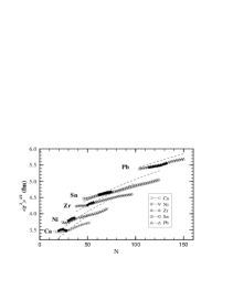
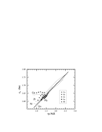
Figure 21: Left: The rms charge radii versus the neutron number $N$ for even-even Ca, Ni, Zr, Sn, Pb isotopes. The RCHB calculation with $\delta$-force is represented by open symbols, while the corresponding data is denoted by solid symbols. The dashed lines represent the predictions by the $A^{1/3}$ law with $r_{A}=1.228$ fm. Right: The experimental (solid symbols) and RCHB predicted (dashed lines) coefficient $r_{Z}=R_{c}/Z^{1/3}$ for the nuclear charge radii as a function of isospin quantity $\eta=N/Z$ in even-even Ca, Ni, Zr, Sn and Pb isotopes. An asymptotic behavior is drawn as a solid line. Taken from Ref. [129].

For even-even Ca, Ni, Zr, Sn and Pb isotopes, the rms charge radii $r_{c}$ obtained from the RCHB theory (open symbols) and the data available (solid symbols) for the even-even Ca, Ni, Zr, Sn and Pb isotopes are given in Fig. 21. The RCHB calculations reproduce the data very well. For a given isotopic chain, an approximate linear $N$ dependence of the calculated rms charge radii $r_{c}$ is clearly seen in Fig. 21, which shows that the variation of $r_{c}$ for a given isotopic chain deviates from both the simple $Z^{1/3}$ dependence and the simple $A^{1/3}$ law (denoted by dashed lines in Fig. 21). Therefore, a strong isospin dependence of nuclear charge radii is necessary for nuclei with extreme $N/Z$ ratio.

In Fig. 21, the data and RCHB predicted $r_{Z}=R_{c}/Z^{1/3}$ for the proton magic isotopes are also presented as a function of $\eta=N/Z$. It is clearly seen that the coefficient $r_{Z}$ increases linearly with $\eta$ (except some deviations due to deformation or shell effects) and the slopes are nearly the same for these isotopic chains. The linear $\eta$ (or isospin $T_{Z}=(N-Z)/2$) dependence of $r_{Z}$ for an isotopic chain may be understood as the effect of the first order perturbation correction of nuclear wave function due to an isospin $T_{Z}$ dependent interaction [147]. Based on the analysis of data in the middle and upper panels of Fig. 20 and RCHB prediction in Fig. 21, the following isospin dependent $Z^{1/3}$ formula for nuclear charge radii has been proposed [129]:

$$R_{c}=r_{Z}\,Z^{1/3}\left[1+b(\eta-\eta^{*})\right],\ \ \ \ \eta=N/Z,$$ (116)

where $\eta^{*}$ is $\eta=N/Z$ for the nuclei along the $\beta$-stability line which can be directly extracted from the nuclear mass formula [16], $r_{Z}=1.631(11)$ fm as obtained in upper right panel of Fig. 20, and $b=0.062(9)$ obtained from the least square fitting.

The analysis of the available data using Eq. (116) with $r_{Z}$ and $b$ thus obtained is displayed in the lower right panel of Fig. 20. The data are reproduced better by Eq. (116) than by Eq. (114). Description of the data with an isospin dependent $A^{1/3}$ formula, $R_{c}=1.228\,A^{1/3}\left[1+0.029(\eta-\eta^{*})\right]$ is also shown in the lower left panel of Fig. 20 for comparison. The parameter for the isospin term is also obtained by least square fitting of the data. It can be seen that this formula describes the data less successfully than Eq. (116).

In Refs. [140, 145], a modified $A^{1/3}$ formula with additional $\sim(N-Z)/A$ and $\sim 1/A$ terms made some successes on describing nuclear charge radius. In addition, this formua was extended with $\sim A^{-2}$ terms [38], which are considered to account for the isospin dependence of charge radii in light nuclei. Based on the fact that $R_{p}Z^{-1/3}$ is approximately a constant, where $R_{p}$ is the rms radius of proton density distribution, a formula for nuclear charge radius was proposed in Refs. [141, 142, 38], $R_{c}=((r_{p}Z^{1/3})^{2}+0.64)^{1/2}$. Detailed analysis of these expressions show: (i) The $Z^{1/3}$ dependence is a better approximation to available $R_{c}$ data than the $A^{1/3}$ one;(ii) The simple $Z^{1/3}$ dependent formula (114) gives nearly the same result as the formula suggested in Refs.  [141, 142]; (iii) The new isospin dependent $Z^{1/3}$ formula is better than the two-parameter isospin dependent $A^{1/3}$ formula but less better than the three-parameter one. A better agreement of the isospin dependence $Z^{1/3}$ formula of charge radii can be achieved by fitting both $r_{Z}$ and $b$ simultaneously. While in Eq. (116), the same $r_{Z}$ is used as that in Eq. (114), which are derived only from the most stable nuclei. Thus the second term in Eq. (116) mainly corresponds to the isospin dependence of charge radii for the nuclei away from the $\beta$ stability line. It is expected that the modified $Z^{1/3}$ formula (116) will become more useful with more and more data obtained for the nuclei far from the $\beta$-stability line.

4.2.4 Density distribution and cross section

The measurement of interaction cross sections plays an important role in exploring the properties of exotic nuclei because it can provide information of the nuclear density distribution and nuclear radii. Based on the measurement of interaction cross section with radioactive beams at relativistic energy, novel and entirely unexpected features appear: e.g., the neutron halo and skin as the rapid increase in the measured interaction cross-sections in the neutron-rich light nuclei. Systematic investigation of interaction cross sections for an isotope chain or an isotone chain can provide a good opportunity to study the density distributions over a wide range of isospin. From the mean field point of view, the nucleon density distributions in an atomic nucleus determine the mean potential. Since the single particle levels and the shell structure are directly determined by the mean fields, the study of the isospin dependence of shell structure and the mean potential, which become highly diffuse near the particle drip line due to the large diffuseness in the density distribution, is also crucial to understand properties of unstable nuclei. Particularly the study of the surface diffuseness will provide another mean to understand exotic nuclei because the surface diffuseness can be strongly related with the spin-orbital splitting which is mainly determined by the diffuseness in the mean field potentials and could be measured experimentally.

The density distribution and shell structure

Systematic RCHB calculations have been carried out for all the nuclei in Na isotopes with mass number A ranging from 17 to 45 with parameter set NLSH [45]. The calculated binding energies $E_{B}$ and the interaction cross sections with the Glauber Model are shown in Fig. 22. The calculated binding energies $E_{B}$ are in good agreement with the empirical values [89]. The resonance states of ¹⁷Na and ¹⁸Na (with a positive Fermi energy) are exactly reproduced. ¹⁹Na is bound but unstable against the proton emission, reproducing the experimental observation. The neutron drip line nucleus has been predicted to be ⁴⁵Na. The difference between the calculations and the empirical values for the stable isotopes is from the deformation [45].

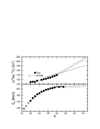
Figure 22: Upper: The interaction cross sections $\sigma_{I}$ of ^ANa isotopes on a carbon target at $950A$ MeV: the open circles are the result of RCHB and the available experimental data ($A=20-23,25-32$) are given by solid circles with error bars. The dashed line is a simple extrapolation based on the RCHB calculation for ^28-31Na. Lower: Binding energies for Na isotopes, the convention is the same as the upper part, but the RCHB result for particle unstable isotopes are indicated by triangle. Taken from Ref. [45].

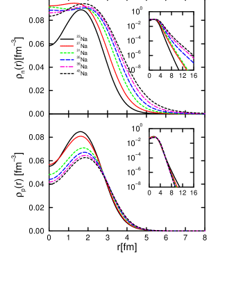
Figure 23: The neutron (upper) and proton (lower) density distributions in Na isotopes. The same figures but in logarithm scale are given as inserts to show the tail part of the density distribution. Taken from Ref. [45].

The density distributions are examined and the relation between the development of halo and shell effect within the RCHB theory is also studied in detail for Na isotopes [45]. For example, the density distributions for both the proton and the neutron in Na isotopes are given in Fig. 23. As seen in the upper part of Fig. 23, the change of the neutron density is as follows: for the nucleus with less neutrons (N), the density at the center is low and it spreads only to some smaller distance. With the increase of N, the density near the center increases due to the occupation of the $2s_{1/2}$ level, so does the development of neutron radius. In the lower part of Fig. 23, the proton density shows different behavior. The surface is more or less unchanged because of the Coulomb Barrier, but with the increase of N, the density of the center decreases due to the slight increasing at the tail. This is due to the symmetry energy. But as the density must be multiplied by a factor $4\pi r^{2}$ before the integration in order to give the fixed Z, the big change in the center does not influence the outer part of the proton distribution very much.

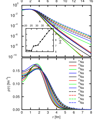
Figure 24: The same as Fig. 23 but for matter density distribution. The upper part is given in logarithm scale (the radius is labeled at the top of the figure) and the radius $r_{0}$ at which $\rho(r_{0})=10^{-4}$ for different isotopes is given as inserts. Taken from Ref. [45].

The matter densities for the even Na isotopes are given in Fig. 24 where the shortest tail in the total density occurs for ^23-25Na, the most stable ones. For either the proton or the neutron rich sides, the tail density increases monotonically. The tail ($r>10$ fm) of the proton rich nuclei is mainly due to the contribution of the proton and that of the neutron drip line nuclei is mainly due to the contribution of the neutron. Compared with the neutron-rich isotopes, the proton distribution for nucleus with less N has higher density at the center, lower density in the middle ($2.5<r<4.5$fm), a larger tail in the outer ($r>4.5$ fm) part.

Figure 25: Left: Single particle energies for neutrons in the canonical basis as a function of the mass number. The dashed line indicates the chemical potential. Right: The occupation probabilities in the canonical basis for ³⁵Na. Taken from Ref. [45].

It is found that there is interesting connections between the matter distribution and the single particle level distribution (see Fig. 25): after ²⁵Na, as it is a sub-closure shell for the $1d_{5/2}$, the neutrons are filled in the $2s_{1/2}$ and $1d_{3/2}$. So the tail of the density for ²⁷Na is two order of magnitude larger than ²⁵Na at $r=10$ fm, while the tail of the density from ²⁷Na to ³¹Na is very close to each other. But as more neutrons are filled in, the added neutrons are filled in the next shell $1f_{7/2}$, $2p_{3/2}$ and $2p_{1/2}$. So again two order of magnitude’s increase has been seen from ³¹Na to ³³Na, and then a gradual increase after ³³Na. So it becomes clear that the rapid increase in the cross section is connected with the filling of neutrons in the next shell or sub shell. In the inserts in Fig. 24: the radius $r_{0}$ at which $\rho(r_{0})=10^{-4}$ fm^-3 is given as a function of the mass number to see the relation between the shell effect and matter distribution more clearly. It is very interesting to see a slight decrease of $r_{0}$ from proton drip line to ²⁵Na. The tail of ²⁵Na is the smallest. From ²⁶Na to ³¹Na, one sees a almost constant $r_{0}$. After a jump from ³¹Na to ³²Na, a rapid increasing tendency appears again.

In Figs. 25 , the microscopic structure of the single particle energies in the canonical basis [35, 42] is given. In the left panel of Fig. 25, the single particle levels in the canonical basis for the isotopes with an even neutron number are shown. Going from $A=19$ to $A=45$ we observe a big gap above the $N=8$, $N=20$ major shell , and $N=14$ sub-shell. The $N=28$ shell for stable nuclei fails to appear, as the $2p_{3/2}$ and $2p_{1/2}$ come so close to $1f_{7/2}$. When $N\geq 20$, the neutrons are filled to the levels in the continuum or weakly bound states in the order of $1f_{7/2}$, $2p_{3/2}$, $2p_{1/2}$, and $1f_{5/2}$. In the right part, the occupation probabilities in the canonical basis of all the neutron levels below $E=10$ MeV have been given for ³⁵Na to show how the levels are filled in nuclei near the drip line.

The surface diffuseness and the spin-orbital splitting

The RCHB theory has also been used to systematically study the tin isotopes from proton drip line to neutron drip line [124]. The spin-orbital splitting

$$E_{ls}=\displaystyle\frac{E_{lj=l-1/2}-E_{lj=l+1/2}}{2l+1}$$ (117)

versus A for the whole isotope chain is given in Fig. 26 for the neutron spin-orbital partners ($1d_{3/2},1d_{5/2}$),($1g_{7/2},1g_{9/2}$), ($1i_{11/2},1i_{13/2}$), ($1p_{1/2},1p_{3/2}$), ($1f_{5/2},1f_{7/2}$), and ($1h_{9/2},1h_{11/2}$), and the proton spin-orbital partners ($1d_{3/2},1d_{5/2}$), and ($1f_{5/2},1f_{7/2}$). It is very interesting to see that the spin-orbital splitting for the neutron and proton is very close to each other, at least for ($1d_{3/2},1d_{5/2}$), and ($1f_{5/2},1f_{7/2}$) cases. The splitting decreases monotonically from the proton drip line to the neutron drip line for all the partners. To see the underlying reason of this behavior, it is very helpful to examine the origin of the spin-orbital splitting in the Dirac equation. The equation of motion for the nucleon moving in scalar and vector potentials could be de-coupled and reduced for the upper component and the lower component, respectively. If it is reduced in the lower component, it will be related with another interesting topic — the pseudo-spin symmetry discussed in next subsection. As for the spin-orbital splitting, the Dirac equation can be reduced for the upper component as the following:

$$[\frac{d^{2}}{dr^{2}}-\frac{1}{E+2M-V+S}\frac{d(2M-V+S)}{dr}\frac{d}{dr}]G^{lj}_{i}(r)$$

$$- [\frac{\kappa(1+\kappa)}{r^{2}}-\frac{1}{E+2M-V+S}\frac{\kappa}{r}\frac{d(2M-V+S)}{dr}]G^{lj}_{i}(r)$$

$$= - (E+2M-V+S)(E-V-S)G^{lj}_{i}(r),$$ (118)

where

$$\kappa=\left\{\begin{array}[]{cc}-l-1&j=l+1/2,\\ l&j=l-1/2.\end{array}\right.$$ (121)

The spin-orbital splitting is due to the corresponding spin-orbital potential

$$\frac{1}{E+2M-V+S}\frac{\kappa}{r}\frac{d(2M-V+S)}{dr}$$ (122)

with some proper normalization factor. It is seen that the spin-orbital splitting in RMF is energy dependent and they depends on the derivative of the potential $2M-V+S$ as well as the particle distribution. Therefore one can introduce the so-called spin-orbital potential: $V_{ls}=\displaystyle\frac{\kappa}{r}\frac{d(2M-V+S)}{dr}$. The $V_{ls}$ for ¹¹⁰Sn, ¹⁴⁰Sn, and ¹⁷⁰Sn, are given in the left panel of Fig. 27. The $V_{ls}$ for both proton and neutron are almost the same, as the potential $V-S$ is a big quantity ($\sim 700$ MeV), the isospin dependence in the spin-orbital potential could be neglected. Therefore the proton and neutron $V_{ls}$ are the same in the present model. That is the reason why the spin-orbital splitting for the neutron and proton is very close to each other in Fig. 26. From ¹¹⁰Sn to ¹⁷⁰Sn, the amplitude of $V_{ls}$ decreases monotonically due to the surface diffuseness. Neutron potentials $V-S$ for ¹⁰⁰Sn, ¹¹⁰Sn,¹²⁰Sn, ¹³⁰Sn, ¹⁴⁰Sn,¹⁵⁰Sn, ¹⁶⁰Sn, and ¹⁷⁰Sn are given in the right panel of Fig. 27 and its inserted figure gives the radii $R_{0}$ at which $V-S=100$ MeV as a function of the mass number. As seen in the above equations, the spin-orbital splitting is related with the derivative of the potential $V-S$ . The surface diffuseness happens for both the vector and scalar potential, as well as for $V-S$ and $V+S$.

Figure 26: The neutron spin-orbit splitting $E_{ls}=\displaystyle\frac{E_{lj=l-1/2}-E_{lj=l+1/2}}{2l+1}$ versus the mass number $A$ in tin isotopes for neutron ($1d_{3/2},1d_{5/2}$), ($1g_{7/2},1g_{9/2}$), ($1i_{11/2},1i_{13/2}$), ($1p_{1/2},1p_{3/2}$), ($1f_{5/2},1f_{7/2}$), and ($1h_{9/2},1h_{11/2}$) orbital and proton ($1d_{3/2},1d_{5/2}$), and ($1f_{5/2},1f_{7/2}$) orbital, respectively. Taken from Ref. [124].

For the decline of the spin-orbital splitting, it comes from the diffuseness of the potential or the outwards tendency of the potential. The diffuseness of the neutron potentials $V+S$ are given in the left panel of Fig. 28 for ¹¹⁰Sn, ¹²⁰Sn, ¹³⁰Sn, ¹⁴⁰Sn, ¹⁵⁰Sn, ¹⁶⁰Sn, and ¹⁷⁰Sn. It is seen that the depth of the potential decreases monotonically from the proton drip line to the neutron drip line and the surface of the potential moves outwards. The inserted figure gives the radii $R_{0}$ at which $V+S=-10$ MeV as a function of the mass number. The proton potentials $V+S$ for ¹¹⁰Sn,¹²⁰Sn, ¹³⁰Sn, ¹⁴⁰Sn,¹⁵⁰Sn, ¹⁶⁰Sn, and ¹⁷⁰Sn are given in the right panel of Fig. 28. With the increase of the neutron number, the proton potentials are pushed towards outside as well due to the proton-neutron interaction.

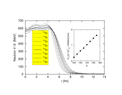
Figure 27: Left: The derivative of the neutron potentials $V(r)-S(r)$ for ¹¹⁰Sn, ¹⁴⁰Sn, and ¹⁷⁰Sn; Right: The neutron potentials $V(r)-S(r)$ for ¹⁰⁰Sn, ¹¹⁰Sn,¹²⁰Sn, ¹³⁰Sn, ¹⁴⁰Sn,¹⁵⁰Sn, ¹⁶⁰Sn, and ¹⁷⁰Sn. In order to examine the surface diffuseness more clearly, the radii $R_{0}$ at which $V(R_{0})-S(R_{0})=100$ MeV has been given as an inserted figure. Taken from Ref. [124].

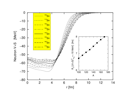
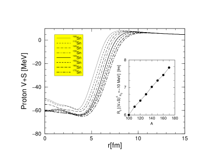
Figure 28: Left: The neutron potentials $V(r)+S(r)$ for ¹⁰⁰Sn, ¹¹⁰Sn,¹²⁰Sn, ¹³⁰Sn, ¹⁴⁰Sn,¹⁵⁰Sn, ¹⁶⁰Sn, and ¹⁷⁰Sn. In order to examine the surface diffuseness more clearly, the radii $R_{0}$ at which $V(R_{0})+S(R_{0})=-10$ MeV has been given as an inserted figure; Right: The proton potentials $V(r)+S(r)$ for ¹¹⁰Sn,¹²⁰Sn, ¹³⁰Sn, ¹⁴⁰Sn,¹⁵⁰Sn, ¹⁶⁰Sn, and ¹⁷⁰Sn. In order to examine the surface diffuseness more clearly, the radii $R_{0}$ at which $V(R_{0})+S(R_{0})=-10$ MeV has been given as an inserted figure. Taken from Ref. [124].

Interaction cross sections

For medium and high energy reactions, the interaction cross section $\sigma_{\rm int}$ can be calculated with the Glauber model which is based on the individual nucleon-nucleon collisions in the overlap volume of the high energy colliding nuclei. In the framework of this model, the nucleus-nucleus reaction cross section can be obtained from nucleon-nucleon reaction cross section. Consider the collision of a projectile nucleus $P$ on a target nucleus $T$ when the nuclei $P$ and $T$ are situated at an impact parameter $\bf b$ relative to each other, the total reaction cross section can be written as

$$\sigma=2\pi\int bdb\left(1-T(b)\right),$$ (123)

where $T(b)$ is the transparency function describing the probability that the projectile will pass through the target without interacting. $T(b)$ is given by

$$T(b)=\exp\left[-\sigma_{NN}\int\rho_{P}({\bf b}_{P},z_{P})d{\bf b}_{P}dz_{P}\,\,\rho_{T}({\bf b}_{T},z_{T})d{\bf b}_{T}dz_{T}\,\,t({\bf b-b_{P}+b_{T}})\right],$$ (124)

where $\sigma_{NN}$ is the nucleon-nucleon reaction cross section suitably averaged over the interacting $n$-$n$, $p$-$p$, and $n$-$p$ pairs [148, 149]. The profile function $t({\bf b})$ for the NN scattering is taken as a delta function for zero-range nuclear interaction.

To compare the cross section directly with experimental measured values, the densities $\rho_{n,p}(r)$ of the target ¹²C and the Na isotopes obtained from RCHB (see Fig. 23) were used in the Glauber model calculation. The cross sections for reaction of Na isotopes at $950A$ MeV on ¹²C have been compared with the experimental values [150] in the upper part of Fig. 22. The agreement between the calculated results and measured ones are fine. The cross section below ²²Na changes only slightly with the neutron number, which means the proton density has played an important role to remedy the contribution of less neutron. From ²⁵Na to the neutron drip line, a gradual increase of the cross section has been observed. After ³²Na, although no data exist yet, a relatively fast increase has been predicted. In short, the measured cross section shows similar behavior as that of RCHB.

Charge changing cross section

Systematic investigation of interaction cross sections for an isotope chain or an isotone chain can provide a good opportunity to study the density distributions over a wide range of isospin [150, 45]. However the contribution from proton and neutron are coupled in the measurement of interaction cross section. To investigate possible differences in proton and neutron density distributions, a combined analysis of the interaction cross section and other experiment on either proton or neutron alone are necessary. The charge-changing cross section which is the cross section for all processes which result in a change of the atomic number for the projectile can provide good opportunity for this purpose. In Ref. [151], the total charge-changing cross section $\sigma_{\rm cc}$ for the light stable and neutron-rich nuclei at relativistic energy on a carbon target were measured. The charge changing cross section $\sigma_{\rm cc}$ are calculated by using the Glauber Model and the proton density of projectiles and total density of target provided by RCHB theory [46].

Figure 29: The proton density distributions predicted by RCHB for the nuclei ^10-22C, ^12-24N, ^14-26O and ^16-25F in logarithm scale. Taken from Ref. [46].

The proton density distributions predicted by RCHB for the nuclei ^10-22C,^12-24N,^14-26O and ^16-25F are given in Fig. 29 in logarithm scale. The change in the density distributions for each isotope chain in Fig. 29 occurs only at the tail or in the center part. The density is multiplied by a factor $4\pi r^{2}$ before an integration in order to get proton number or radii, therefore the change of density in the central region does not matter very much. What is important is the density distribution in the tail part. Compared with the cases of neutron-rich isotopes, the proton distribution of nuclei with less $N$ has higher density in the center, lower density in the middle part ($2.5<r<4.5$fm), a larger tail in the outer part ($r>4.5$ fm) which gives rise to the increase of $r_{\rm p}$ and $\sigma_{\rm cc}$ for the proton rich nuclei as will be seen in following figures.

Figure 30: The total charge-changing cross sections $\sigma_{\rm cc}$ of the nuclei ^10-22C,^12-24N,^14-26O and ^16-25F on a carbon target at relativistic energy. The open circles are the result of RCHB and the available experimental data are given by solid circles with error bars. Taken from Ref. [46].

With the proton density from RCHB calculations for the projectile used for $\rho_{P}({\bf b}_{P},z_{P})$ in Eq. (124), the total charge-changing cross sections $\sigma_{\rm cc}$ of the nuclei ^10-22C, ^12-24N, ^14-26O and ^16-25F on a carbon target at relativistic energy are calculated and given in Fig. 30. The results of the Glauber model are represented by open circles and available data [151] by solid ones with error bars. The agreement between the calculation and the measurement is very good.

The charge changing cross sections change only slightly with the neutron number except for proton-rich nuclei. This indicates that the proton density plays an important role in determining the charge-changing cross sections $\sigma_{\rm cc}$. A gradual increase of the cross section can be observed towards the neutron drip line. However, the big error bars of the data cannot help to conclude anything here yet. It is shown clearly that the RCHB theory, when combined with the Glauber model, can provide reliable description for not only interaction cross section but also charge changing cross section. From comparison between Fig. 30 and Fig. 17, one finds similar trends of variations of proton radii and of charge changing cross sections for each isotope chain which implies again the important role that proton plays in determining the charge-changing cross sections.

4.3 Single particle levels and pseudospin symmetry

The concept of pseudo-spin is that the single particle orbitals with $j=l+1/2$ and $j=(l+2)-1/2$ lie very close in energy and can therefore be labelled as pseudo-spin doublets with quantum number $\tilde{n}=n-1$, $\tilde{l}=l-1$, and $\tilde{s}=s=1/2$. This concept is originally found in spherical nuclei [28, 29] , but later proved to be a good approximation in deformed nuclei as well [152, 153, 154]. It is shown that pseudo-spin symmetry remains an important physical concept even in the case of triaxiality [155]. The origin of pseudo-spin is proved to be connected with the special ratio in the strength of the spin-orbit and orbit-orbit interactions [156, 157] and the unitary operator performing a transformation from normal spin to pseudo-spin space have been discussed [156, 157, 158]. However, it is not explained why this special ratio is allowed in nuclei.

The relation between the pseudo-spin symmetry and the RMF theory was first noted in Ref. [159], in which Bahri et al found that the RMF explains approximately the strengthes of spin-orbit and orbit-orbit interactions found by non-relativistic calculations. More details have been given in Refs. [160, 153], in which it was suggested that the origin of pseudo-spin is related to the strength of the scalar and vector potentials. Ginocchio first revealed that pseudo-orbital angular momentum is nothing but the “orbital angular momentum” of the lower component of the Dirac wave function [30].

In the Dirac equation of the nucleon, when the scalar potential $S(\mathbf{r})$ and the vector potential $V(\mathbf{r})$ are equal in amplitudes but opposite in sign, i.e., $S(\mathbf{r})+V(\mathbf{r})=0$, or more generally, $d[S(\mathbf{r})+V(\mathbf{r})]/dr=0$, there is an exact pseudospin symmetry in single particle spectra [30, 31, 32]. Under these conditions, there should be some special relations between the four components of the Dirac wave functions of the pseudospin doublets which have been used to test the pseudospin symmetry in realistic nuclei [161, 162, 163, 164].

The pseudo spin symmetry in deformed nuclei has also been extensively studied in the framework of the RMF model. The conditions for an exact pseudo spin symmetry and the relationships for the lower components of the Dirac eigenfunctions were investigated in Refs. [165, 166, 167, 168]. The relationships between the upper and lower components of the two states in the pseudo spin doublets have been studied thoroughly for realistic deformed relativistic eigenfunctions [164, 169].

There are also many other investigations on the pseudo-spin symmetry in the framework of RMF theory [170, 171, 172, 173, 174, 175, 176, 177]. A thorough review is certainly beyond the purpose of the present paper. In the following, the pseudo-spin symmetry in RCHB theory will be briefly reviewed.

From the radial Dirac equation for spherical nuclei, similar as Eq. (118), one can derive the radial equation for the lower components:

$$[\frac{d^{2}}{dr^{2}}+\frac{1}{E-V-S}\frac{d(V+S)}{dr}\frac{d}{dr}]F^{lj}_{i}(r)+[\frac{\kappa(1-\kappa)}{r^{2}}-\frac{1}{E-V-S}\frac{\kappa}{r}\frac{d(V+S)}{dr}]F^{lj}_{i}(r)$$ (125)

$$= -(E+2M-V+S)(E-V-S)F^{lj}_{i}(r),$$

where $\kappa(\kappa-1)=\tilde{l}(\tilde{l}+1)$. It is clear that one can use either Eq. (125) or equivalently Eq. (118) to get the eigenvalues $E$ and the corresponding eigenfunctions. In Section 4.2.4, Eq. (118) has been used to discuss the spin-orbital splitting in connection with the corresponding spin-orbital potential. If the Eq. (125) is used instead and the pseudo spin-orbital potential (PSOP) term, $\displaystyle\frac{1}{E-V-S}\frac{\kappa}{r}\frac{d(V+S)}{dr}$, is neglected, then the eigenvalues $E$ for the same $\tilde{l}$ will degenerate. This is the phenomenon of pseudo-spin symmetry observed in Refs. [28, 29]. As shown in Ref. [43], the particle levels for the bound states in canonical basis are the same as those by solving the Dirac equation with the scalar and vector potentials from RCHB. Therefore Eqs. (118) and (125) remain the same in canonical basis even after the pairing interaction has been taken into account.

In Eq. (125), the term which splits the pseudo-spin partners is simply the PSOP. The hidden symmetry for the pseudo-spin approximation is revealed as $d(V+S)/dr=0$, which is more general and includes $V+S=0$ discussed in [30] as a special case. For exotic nuclei with highly diffuse potentials, $d(V+S)/dr\sim 0$ may be a good approximation and then the pseudo-spin symmetry will be good. But generally, $d(V+S)/dr=0$ is not always satisfied in the nuclei and the pseudo-spin symmetry is an approximation. However, if $|\displaystyle\frac{1}{E-V-S}\frac{\kappa}{r}\frac{d(V+S)}{dr}|\ll|\displaystyle\frac{\kappa(1-\kappa)}{r^{2}}|$, the pseudo-spin approximation will be good. Thus, the comparison of the relative magnitude of the pseudo centrifugal barrier (PCB), $\displaystyle\frac{\kappa(1-\kappa)}{r^{2}}$, and the PSOP can provide us with some information on the pseudo-spin symmetry. In Ref. [31], with the scalar and vector potentials derived from a self-consistent RCHB calculation, the pseudo-spin symmetry and its energy dependence have been discussed in realistic nuclei. Afterwards, the pseudo-spin splitting for exotic nuclei in Zr and Sn isotopes has been studied [32].

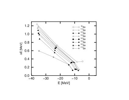
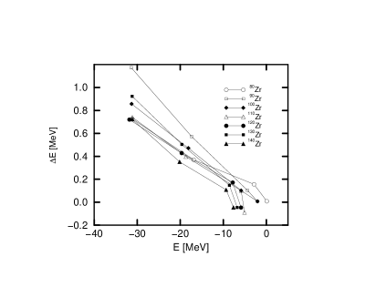
Figure 31: The pseudo-spin orbit splitting $\displaystyle\Delta E=\frac{E_{\tilde{l}j=\tilde{l}-1/2}-E_{\tilde{l}j=\tilde{l}+1/2}}{2\tilde{l}+1}$ versus the binding energy $\displaystyle E=\frac{\tilde{l}E_{\tilde{l}j=\tilde{l}+1/2}+(\tilde{l}+1)E_{\tilde{l}j=\tilde{l}-1/2}}{2\tilde{l}+1}$ for Zr and Sn isotopes. From left to right, the pseudo-spin partners correspond to ($1d_{3/2},2s_{1/2}$), ($1f_{5/2},2p_{3/2}$), ($1g_{7/2},2d_{5/2}$) and ($2d_{3/2},3s_{1/2}$), respectively. Taken from Ref. [31].

The redefined pseudo-spin orbital splitting $\displaystyle\Delta E=\frac{E_{\tilde{l}j=\tilde{l}-1/2}-E_{\tilde{l}j=\tilde{l}+1/2}}{2\tilde{l}+1}$ versus the average single particle energy $\displaystyle E=\frac{\tilde{l}E_{\tilde{l}j=\tilde{l}+1/2}+(\tilde{l}+1)E_{\tilde{l}j=\tilde{l}-1/2}}{2\tilde{l}+1}$ for the bound pseudo-spin partners in Sn and Zr isotopes are plotted in Fig. 31. In both isotopes, a monotonous decreasing behavior with the decreasing binding energy is clearly seen. The pseudo-spin splitting for $3s_{1/2}$ and $2d_{3/2}$ is more than $10$ times smaller than that of the $2s_{1/2}$ and $1d_{3/2}$. As far as the isospin dependence of the pseudo-spin orbital splitting is concerned, the splitting in Sn isotopes gives a monotonous decreasing behavior with the increasing isospin. Particularly for $2s_{1/2}$ and $1d_{3/2}$ partners, the pseudo-spin splitting in ¹⁷⁰Sn is only half of that in ⁹⁶Sn. Just as one expects [31], the pseudo-spin symmetry in neutron-rich nuclei is better. In Zr isotopes, although the situation is more complicated (e.g., the effect of the deformation which is neglected here), the pattern is more or less the same, i.e., a monotonous decreasing behavior with the decreasing binding energy and a monotonous decreasing behavior with the isospin. From these studies, the pseudo-spin symmetry remains a good approximation for both stable and exotic nuclei. A better pseudo-spin symmetry can be expected for the orbital near the threshold, particularly for nuclei near the particle drip line.

Figure 32: The comparison of the effective pseudo centrifugal barrier (PCB) $\displaystyle(E-V-S)\frac{\kappa(\kappa-1)}{r^{2}}$ (dashed lines and dot-dashed lines) and the effective pseudo-spin orbital potential (PSOP) $\displaystyle\frac{\kappa}{r}\frac{d(V+S)}{dr}$ (solid line ) in arbitrary scale for $d_{3/2}$ (upper) and $s_{1/2}$ (lower) in ¹²⁰Zr. The dashed lines are for $1d_{3/2}$ and $2s_{1/2}$, and the dot-dashed lines are for $2d_{3/2}$ and $3s_{1/2}$. The inserted boxes show the same quantities, but the ordinate is magnified and the abscissa is reduced to show the behaviors of the effective PCB and the effective PSOP near the nuclear surface. Taken from Ref. [31].

To understand why the energy splitting of the pseudo-spin partner changes with different binding energies and why the pseudo-spin approximation is good in RMF, the PSOP and PCB should be examined carefully. Unfortunately, it is very hard to compare them clearly, as the PSOP has a singularity at $E\sim(V+S)$. As one is only interested in the relative magnitude of the PCB and the PSOP, the effective PCB, $\displaystyle(E-V-S)\frac{\kappa(\kappa-1)}{r^{2}}$, and the effective PSOP, $\displaystyle\frac{\kappa}{r}\frac{d(V+S)}{dr}$ are introduced for comparison. They correspond to the PCB and the PSOP multiplied by a common factor $E-V-S$ respectively.

Figure 33: The comparison of the effective pseudo centrifugal barrier (PCB) $\displaystyle(E-V-S)\frac{\kappa(\kappa-1)}{r^{2}}$ (dashed lines) and the effective pseudo-spin orbital potential (PSOP) $\displaystyle\frac{\kappa}{r}\frac{d(V+S)}{dr}$ (solid line ) multiplied by the square of the wave function $F$ of the lower components in arbitrary scale for $d_{3/2}$ (upper) and $s_{1/2}$ (lower) in ¹²⁰Zr. Taken from Ref. [31].

The effective PSOP does not depend on the binding energy of the single particle level, but depends on the angular momentum and parity. On the other hand the effective PCB depends on the energy. Comparing these two effective potentials one could see the energy dependence of the pseudo-spin symmetry. They are given in Fig. 32 for $s_{1/2}$ (lower) and $d_{3/2}$ (upper) of ¹²⁰Zr in arbitrary scale.

The pseudo-spin approximation is much better for the less bound pseudo-spin partners, because the effective PCB is smaller for the more deeply bound states. This is in agreement with the results shown in Fig. 31. The effective PSOP and the effective PCB are also given as inserts in Fig. 32 in order to show their behavior near the nuclear surface.

The effective PCB (dashed lines or dot-dashed lines) and the effective PSOP (solid lines) multiplied by the squares of the lower component wave function $F(r)$ are given in Fig. 33, for $2s_{1/2}$ (upper left), $3s_{1/2}$ (lower left), $1d_{3/2}$ (upper right), and $2d_{3/2}$ (lower right) of ¹²⁰Zr in arbitrary scale. The pseudo-spin approximation is much better for the less bound pseudo-spin partners, because the effective PCB is smaller for the more deeply bound states. This is in agreement with the results shown above. It is clear that the contribution of the effective PCB (dashed lines or dot-dashed lines) is much bigger than that of the effective PSOP (solid lines). Generally the effective PSOP is two orders of magnitude smaller than the effective PCB. The energy difference between the orbital $j=\tilde{l}+1/2$ and the orbital $j=\tilde{l}-1/2$ is always negative with some exceptions. Further investigations reveal that the integration of $\dfrac{d(V+S)}{dr}|F|^{2}$ over $r$ gives the splitting of the pseudo-spin partners, whose sign will decide the normal splitting or the reverse.

4.4 Halos and giant halos

Since the experimental discovery of neutron halo phenomena in ¹¹Li [13], the study of exotic nuclei has become a very challenging topic in nuclear physics. Experimentally more and more halo nuclei have been observed [6, 7, 8, 11, 12, 178, 179, 180, 181]. On the theoretical side very different models have been used to describe these phenomena. Three-body calculations based on an inert core of ⁹Li and two outside neutrons treat the translational invariance properly, but they neglect polarization effects. Full shell model calculations contain all the configuration mixing, but they are limited to relatively small configuration spaces in the oscillator model. In the mean field description, the large radius observed experimentally in ¹¹Li has been interpreted by the fact that filling in more and more neutrons in the nuclear well, the Fermi surface for the neutrons comes close to the continuum limit. Due to the small single-neutron separation energy, the tails of the two wave functions of the last filled orbital (1$p_{1/2}$) reach very far outside of the nuclear well and a neutron halo is formed [13]. Although this simple interpretation is based on the mean field picture, several microscopic theoretical investigations within self-consistent mean field models [182, 183, 184, 185] have failed. In fact, it would be a strange accident if the last occupied neutron level in ¹¹Li, the 1$p_{1/2}$ orbit, would be so close to the continuum limit that the tail of the last two uncorrelated neutron wave functions reaches so far out as would be necessary to reproduce the large experimental radius observed. Therefore, in the non-relativistic scheme Bertsch et al [182] and Sagawa [184] introduced an artificial modification to the potential in order to reproduce the small separation energy in their mean field calculations using Skyrme interactions. In this way the authors were able to reproduce qualitatively the observed trends, although some discrepancies still remained.

Koepf et al [183] were the first to investigate the neutron halo in the RMF theory for both spherical and axially deformed cases. They found large deformations for the lighter Li isotopes, but a spherical shape for ¹¹Li and as in the non-relativistic investigations the binding energy of the 1$p_{1/2}$ was too large so as to reproduce a neutron halo. Zhu et al [185] improved the result of the RMF calculations by applying a similar modification to the potential as in Ref. [184] in order to adjust the proper size of the halo.

The first self-consistent microscopic description of the halo in ¹¹Li was achieved by using the RCHB theory where the pairing correlations are taken into account by a density dependent force of zero range and the halo was reproduced in a self-consistent way by using the scattering of Cooper pairs to the 2s_1/2 level in the continuum [36].

In Ref. [121], pairing correlations and the coupling to particle continuum states are described by finite range two-body forces and the finite element method are used in the coordinate space discretization of the coupled system of Dirac-Hartree-Bogoliubov integro-differential eigenvalue equations, and Klein-Gordon equations for the meson fields [71]. The authors of Ref. [121] performed calculations for the isotopic chains of Ne and C nuclei and found evidence for the occurrence of neutron halo in heavier Ne isotopes. The RHB theory is also applied to the description of the properties of light nuclei in isotopic chains of C, N, O, F, Ne, Na, and Mg with large neutron excess in Ref. [186]. The RHB model predicts the formation of neutron skin and eventually a neutron halo in Ne and Na due to the quasi-degeneracy of the triplet of states 1f_7/2, 2p_3/2, and 2p_1/2 which are close to the Fermi surface in neutron rich nuclei.

To describe medium-heavy nuclei far from the $\beta$ stability line, the main problem of nuclear structure models is the extrapolation of effective forces to nuclei with extreme isospin values because most of these nuclei are still not accessible experimentally and therefore one could not compare theoretical results with empirical data. In order to make predictions for medium-heavy nuclei at the neutron drip line, one has to test available effective interactions in detailed calculations of the properties of neutron-rich nuclei for which a comparison with experimental data is possible. This has been done in Ref. [187] where the RHB theory is applied in the description of the ground-state properties of Ni and Sn isotopes. In a comparison with available experimental data, it is shown that the NL3 + Gogny D1S effective interaction provides an excellent description of binding energies, neutron separation energies, and proton and neutron rms radii. The results indicate that this choice of model parameters might also be valid for nuclei with more extreme isospin values, i.e., medium-heavy nuclei at the drip lines.

We note that the RHB model solved in a discretized coordinate space is available only for spherical systems up to now. The deformed RHB theory solved in a harmonic oscillator basis [188] is not applicable for halo nuclei due to the localization property of the harmonic oscillator potential. One should work in two or three dimensional spatial lattice or instead, one can improve the asymptotic behavior of the HO wave function [64, 65] or adopt other basis which has a correct asymptotic behavior [73].

In the following, we will briefly review the RCHB description of halo phenomena and the prediction of giant halo in light and medium-heavy nuclei.

4.4.1 Neutron halo in light nuclei

The ground state properties of Li isotopes with mass numbers $A=6$ to $A=11$ were investigated by using the RCHB theory with the effective interaction NL2 [36]. Pairing is neglected for the three protons and the strength $V_{0}$ of the pairing force (96) for the neutrons is determined by a calculation in the nucleus ⁷Li adjusting the corresponding pairing energy -$\displaystyle\frac{1}{2}\mbox{Tr}\ \Delta\kappa$ to that of a RHB-calculation in an oscillator basis using the finite range part of the Gogny force D1S of Ref. [119] in the pairing channel. Good agreement with experimental values is found for the total binding energies and the radii of the isotope chain ⁶Li to ¹¹Li. The matter radius shows a considerable increase when going from the nucleus ⁹Li to ¹¹Li. In contrast to the earlier mean field calculations of Refs. [182, 184, 185] these results are obtained without any artificial modifications of the potential.

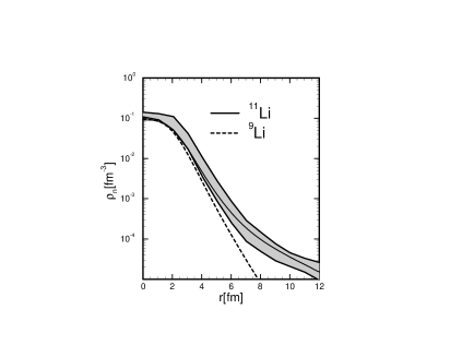
Figure 34: Calculated and experimental density distribution in ¹¹Li and ⁹Li. The solid line shows the result of ¹¹Li while the dashed line corresponds to the calculation of ⁹Li. The shaded area gives the experimental results with error bars. Taken from Ref. [36].

In Fig. 34 the corresponding density distribution for the neutrons in the isotopes ⁹Li and ¹¹Li is shown. It is clearly seen that the increase of the matter radius is caused by a large neutron halo in the nucleus ¹¹Li. Its density distribution is in very good agreement with the experimental density of this isotope shown with its error bars by the shaded area.

Figure 35: The mean field potential $S+V$ for protons (l.h.s.) and neutrons (r.h.s.). The chemical potential is given by a dashed line. The energy levels in the canonical basis are indicated by horizontal lines with various lengths proportional to the occupation of the corresponding orbit. Taken from Ref. [36].

In order to understand the microscopic structure of this halo, in Fig. 35 the mean field $S(r)+V(r)$ for the protons and neutrons together with the energy levels in the canonical basis is shown. The Fermi level for the neutrons is very close to the continuum limit in close vicinity to the $\nu 1p_{1/2}$ and to the $\nu 2s_{1/2}$ level. The length of these energy levels in Fig. 35 is proportional to the corresponding occupation. One clearly finds that pairing correlations cause a partial occupation of both the $\nu 1p_{1/2}$ and the $\nu 2s_{1/2}$ level, i.e. a scattering of Cooper pairs to the continuum.

In contrast to many previous investigations, in the RCHB model, the halo is not formed by two neutrons occupying the $1p_{1/2}$ level very close to the continuum limit, but is formed by Cooper-pairs scattered mainly in the two levels $1p_{1/2}$ and $2s_{1/2}$. This is made possible by the fact that the $2s_{1/2}$ comes down close to the Fermi level in this nucleus and by the density dependent pairing interaction coupling the levels below the Fermi surface to the continuum. The RCHB theory provides a much more general mechanism for halo occurring in nuclei. One needs only several single particle levels with small orbital angular momenta and correspondingly small centrifugal barriers close to, but not necessarily directly at, the continuum limit.

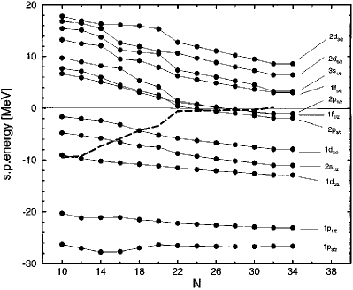
Figure 36: Canonical basis single-particle neutron levels as functions of the number of neutrons. The spectrum is calculated for Ne isotopes. Taken from Ref. [121].

In Ref. [121], the isotopic chains of Ne and C nuclei were studied with the RHB model with finite range pairing interaction in the coordinate space. The formation of neutron skin and eventually a neutron halo in Ne was found to be mainly due to the quasi-degeneracy of the triplet of states 1f_7/2, 2p_3/2, and 2p_1/2. In Fig. 36, the neutron single-particle spectrum in the canonical basis is displayed for Ne isotopes. The energies of levels in the continuum decrease with increasing neutron number (cf. Fig. 41 (a)). The shell structure dramatically changes at $N\geq$ 22. The triplet of states 1f_7/2, 2p_3/2, and 2p_1/2 approaches zero energy, and a gap is formed between these states and all other states in the continuum. The Fermi level uniformly increases toward zero for $N$ = 22. Between $N$ = 22 and $N$ = 32, the Fermi level is practically constant and very close to the continuum. The addition of neutrons in this region of the drip does not increase the binding. Only the spatial extension of neutron distribution displays an increase. At $N$ = 32 the Fermi energy becomes slightly positive, and heavier isotopes are not bound any more. The finite range pairing interaction promotes neutrons from the 1f_7/2 orbital to the 2p levels. Since these levels are so close in energy, the total binding energy does not change significantly. Because of their small centrifugal barrier, the 2p_3/2 and 2p_1/2 orbitals form the halo.

4.4.2 Giant halos in Zr isotopes

In all of the halos observed so far, one has only a very small number of nucleons, namely one or two outside of the normal core. In order to study the influence of correlations and many-body effects it would be very interesting to find also nuclei with a larger number of neutron distributed in the halo. Following the successful description of the halo nucleus ¹¹Li, the RCHB theory was used to study and predict giant neutron halos for Zr-isotopes close to the neutron drip line [43]. It is formed by up to six neutrons outside of the ¹²²Zr core with the magic neutron number $N=82$.

Figure 37: Upper: rms radii for neutrons and protons in Zr isotopes close to the neutron drip line as a function of the mass number $A$. Lower: single particle energies for neutrons in the canonical basis. The dashed line indicates the chemical potential. Taken from Ref. [43].

From the upper panel of Fig. 37 which presents the rms radii of the protons and neutrons for the Zirconium isotopes, one finds a kink for the neutron rms radius at the magic neutron number $N=82$. This kink can be understood more clearly by considering the microscopic structure of the underlying wave functions and the single particle energies in the canonical basis which is shown in the lower panel of Fig. 37. Going from $N=70$ to $N=100$, there is a big gap above the 1$h_{11/2}$ orbit. For $N>82$, the neutrons are filled to the levels in the continuum or weakly bound states in the order of $3p_{3/2}$, $2f_{7/2}$, $3p_{1/2}$, $2f_{5/2}$ and $1h_{9/2}$.

Figure 38: Upper: neutron and proton density distribution in ¹³⁴Zr. Dashed lines indicate calculations for different values of the box size $R$ and the dashed-dotted line give the neutron distribution for the core ¹²²Zr. Lower: relative contributions of the different orbits to the full neutron density as a function of the radius. The shaded area indicates the total neutron density in arbitrary units. Taken from Ref. [43].

The neutron chemical potential is given in this Figure by a dashed line. It approaches rapidly the continuum already shortly after the magic neutron number $N=82$ and it crosses the continuum at $N=100$ for the nucleus to ¹⁴⁰Zr. In this region the chemical potential is very small and almost parallel to the continuum limit. This means that the additional neutrons are added with a very small, nearly vanishing binding energy at the edge of the continuum. The total binding energies $E$ for the isotopes above ¹²²Zr are therefore almost identical. This has been recognized already in Ref. [189] in RMF calculations using the BCS approximation and an expansion in an oscillator basis, which is definitely not reliable for chemical potentials so close to the continuum limit.

In the upper panel of Fig. 38 the density distributions for neutrons and protons in the nucleus ¹³⁴Zr are shown. A very large box size is needed to describe the halo properly. For $R=$30 fm the neutron density is reliably reproduced only up to $r=25$ fm, where it has decreased to 10^-6 fm^-3. The full line in the upper panel of Fig. 38 is an asymptotic extension to infinite box size. On the other hand, the density distribution inside the nucleus is reproduced properly even for small values of the box size. The relative contributions $\rho_{nlj}$ of the different orbits characterized by the quantum numbers $nlj$ with respect to the total neutron density $\rho_{n}$ are displayed in the lower panel of Fig. 38. The shaded area gives the total neutron density in arbitrary units. The halo is formed essentially by contributions from three orbits $3p_{3/2}$, $3p_{1/2}$, and $2f_{7/2}$. The most inner part of the halo ($7\leq r\leq 9$ fm) the $2f_{7/2}$ orbit plays the dominant role. As can be seen in the lower part of Fig. 38, this orbit is slightly below the chemical potential and to the continuum limit in this nucleus. Further outside ($10\leq r\leq 15$ fm) its relative contribution is strongly reduced because of the larger centrifugal barrier felt by the $l=3$ orbit. In this region the orbit $3p_{3/2}$, which has nearly the same position as the $2f_{7/2}$ orbit, takes over. Because of the smaller orbital angular momentum, this orbit feels a reduced centrifugal barrier. For even larger distances from the center ($r\geq 15$ fm) its relative contribution is somewhat reduced and the $3p_{1/2}$ orbit gains importance. The $3p_{3/2}$ and the $3p_{1/2}$ levels feel the same centrifugal barrier, but the latter is situated directly at the continuum limit and therefore it is more loosely bound than the other two orbits.

The occupation probabilities in the canonical basis of all the neutron levels near the Fermi surface, i.e. in the interval $-20\leq E\leq 10$ MeV are presented in Fig. 39 for all the Zr-isotopes between $A=108$ and $A=140$. The chemical potential is indicated by a vertical line. For the mass numbers $A<122$ the chemical potential lies several MeV below the continuum limit ($E=0$) and there is only very little occupation in the continuum ($E>0$). The nucleus ¹²²Zr has a magic neutron number and no pairing. As the neutron number goes beyond this closed core, the occupation of the continuum becomes more and more important. Adding up the occupation probabilities $v^{2}$ for the levels with $E>0$ one finds in the continuum 2 particles for $N=84$, 4 for $N=86$, 6 $N=88$, roughly 3 for $N=90$, roughly 4 for $N=92$, roughly 3 for $N=94$, roughly 4 for $N=96$, roughly 5 for $N=98$, and roughly 6 for $N=100$ (where the neutron drip line is reached).

Figure 39: The occupation probabilities in the canonical basis for various Zr isotopes with mass number A as a function of the single particle energy. The chemical potential is indicated by a vertical line. For $A>122$ the number $N_{h}$ of neutrons in the halo is also shown. Taken from Ref. [43].

Considering the very extended neutron rms radii of these systems and estimating the number of valence neutrons which would fit into the same volume outside the ¹²²Zr core (shown in Fig. 38 by a dashed dotted line) if they would be packed with normal neutron density, one finds for ¹³⁴Zr 24 neutrons instead of 12 and for ¹⁴⁰Zr 34 neutrons instead of 18. This means that the density outside of the ¹²²Zr core is reduced by roughly a factor of 2. This phenomenon is therefore clearly a neutron halo and not a neutron skin. As one sees from Fig. 3 the tail of the density is proportional to $\exp(-2\sqrt{4mS}r)$ with $S\approx 0.4\,$MeV. This fact is also emphasized by the extremely low 2n-separation energies ($<~{}0.5$ MeV) of these systems. This phenomenon is called a Giant Halo because of the large number of particles in the halo region [43]..

4.4.3 Giant halos in lighter nuclei

Although the giant halos were predicted in Zr isotopes, it is very difficult for experimentalists to confirm them because the exotic Zr isotopes with $N>82$ are too heavy to be synthesized by the RIB facilities at present. Thus it is valuable to investigate the giant halo phenomena in lighter nuclei which are experimentally accessible today. Ground state properties of all the even-even O, Ca, Ni, Zr, Sn, Pb isotopes ranging from the proton drip line to the neutron drip line were investigated [44, 126]. The two neutron sepation energies are shown in Fig. 14 where one finds the $S_{2n}$ values for exotic Ca isotopes near neutron drip line are very close to zero in the large mass region, i.e., $S_{2n}\approx 2.06,~{}1.24,~{}0.76,~{}0.43,~{}0.21,~{}0.04$ MeV for $A=62,~{}64,~{}66,~{}68,~{}70,~{}72$ isotopes, respectively. If one regards ⁶⁰Ca as a core, then the several valence neutrons occupying levels above the $N=40$ sub-shell for these $A>60$ exotic nuclei are all weakly bound and can be scattered easily to the continuum levels due to the pairing interaction, especially for ^66-72Ca. This case is very similar to $S_{2n}$ in Zr isotopes with $N>82$ (see Fig. 14) [43] . Note that for Sn isotopes in the vicinity of the drip line [124], however, $S_{2n}$ decrease rather fast with the mass number and for Ni isotopes [42], $S_{2n}$ are quite large ($\sim 2$MeV) and undergo a sudden drop to negative value at the drip line nucleus. Such behavior of $S_{2n}$ in Ca isotopes with $N>40$ indicates that there exist giant halos in these nuclei, just as what happens in Zr isotopes with $N>82$ [43]. From Fig. 18, one also finds similarity between Ca and Zr isotopes: the neutron radius increases suddenly with neutron number increasing in the Ca chain above $N=40$ and in Zr chain above $N=82$. Together with the analysis of nucleon density distributions, single particle levels and the occupation probabilities in the canonical basis, it is predicted that giant halo may exist in Ca isotopes with A$>$60 [44, 126].

Compared with giant halos in Zr chain, the halos in Ca isotopes will be much easier to access with today’s radioactive facilities. This means that the giant halos in the Ca isotopic chain are challenging but promising for experimentalists. In order to make the conclusion more solid and exclude the effects from possible error in $S_{2n}$ ($\sim$ 1 MeV), in Fig. 40, the two-neutron separation energies $S_{2n}$ in drip line region for even-neutron Ne, Na, Mg, and Al chains (left panel) and for Ar, K, Ca, Sc and Ti chains (right panel) are presented. Open symbols represent the values calculated from the RCHB theory with the NLSH parameter set while corresponding filled symbols represent the data available. It should be noted that the calculations are performed by keeping the shape spherical. Nevertheless it can be seen from the figure that all these $S_{2n}$ curves are almost parallel to each other and the zero $S_{2n}$ line. Although the calculated $S_{2n}$ value may differ from the data by 1 or 2 MeV, there must be one or more isotope chains in which many nuclei have the $S_{2n}$ values very close to zero thus are good candidates for giant halos.

Experimentally much efforts have been made to search the drip line for heavier elements. New experiments have shown that both ³⁷Na and ³⁴Ne are bound while ³³Ne and ³⁶Na are missing [190, 191], as expected from the predictions in Ref. [70]. In Fig. 40, ³⁷Na and ³⁴Ne lie in the drip line region and approach the predicted giant halo area. Therefore much more experimental effort should be devoted to measuring their masses and extending the isotope chains for the possible giant halos.

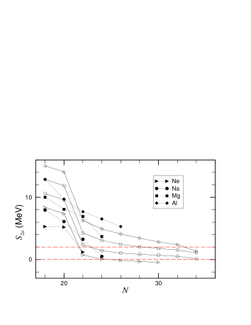
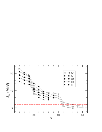
Figure 40: Left: The two-neutron separation energies $S_{2n}$ for even-neutron Ne, Na, Mg, and Al nuclei in the drip line region. Open symbols represent the values calculated with the RCHB theory with the NLSH parameter set, while corresponding solid symbols represent the data available. The horizontal line at 2MeV denotes the upper limit for the possible occurrence of halos. Right: for even Ar, K, Ca, Sc, and Ti nuclei in the drip line region. Taken from Ref. [126].

4.5 Halos in hypernuclei

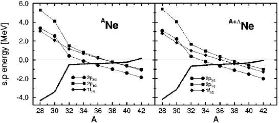
Figure 41: 1f-2p single-particle neutron levels in the canonical basis for the Ne (a), and Ne+$\Lambda$ (b) isotopes. The dotted line denotes the Fermi level. Taken from Ref. [192].

The production mechanisms, spectroscopy, and decay modes of hypernuclear states have been the subject of many theoretical studies. The relativistic Hartree Bogoliubov model in coordinate space with finite range pairing interaction [121, 71] has also been applied to describe $\Lambda$ hypernuclei with a large neutron excess [192]. It is found that the inclusion of the $\Lambda$ hyperon does not produce excessive changes in bulk properties but shifts the neutron drip by stabilizing an otherwise unbound core nucleus at drip line. For example, the nucleus ⁴²Ne was unbound without the $\Lambda$ (see Fig. 41 (a)). The presence of the strange baryon stabilizes the otherwise unbound core and ^42+ΛNe becomes bound (see Fig. 41 (b)). The microscopic mechanism through which additional neutrons are bound to the core originates from the increase in magnitude of the spin-orbit term in presence of the $\Lambda$ particle [192].

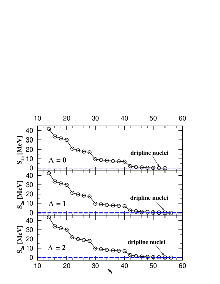
Figure 42: The two-neutron separation energies $S_{2n}$ in even-N Ca isotopes versus the neutron number N. The upper panel is for ordinary nuclei, the middle one for single-$\Lambda$ hyper nuclei, and the lower one for double-$\Lambda$ hyper nuclei. Taken from Ref. [47].

Motivated by experimental knowledge of $\Lambda$-N interaction and theoretical understanding on giant halo [43, 44, 126], it is interesting to observe the possible appearances of halos in hyper exotic nuclei as what have been done in Ref. [47]. In Fig. 42, two neutron separation energies $S_{2n}$ for ordinary nuclei, single-$\Lambda$ hyper nuclei and double-$\Lambda$ hyper nuclei of Ca isotopes labelled by $\Lambda=0$, $\Lambda=1$ and $\Lambda=2$, respectively, from the proton to neutron drip line are presented. It is clear that one or two $\Lambda$ hyperons lower the neutron Fermi level a little bit but keep the neutron shell structure unchanged. Therefore, the neutron drip line is pushed outside from $N=52$ in ordinary isotope chain to $N=54$ in hyper isotope chain. Meanwhile, giant halo due to pairing correlation and the contribution from the continuum still exist in Ca hyper nuclei similar as that in ordinary Ca isotopes [44, 126]. This is a slight but rewarding step for exploring the limit of drip line nuclei on the basis of the giant halo. For more details, see Ref. [47].

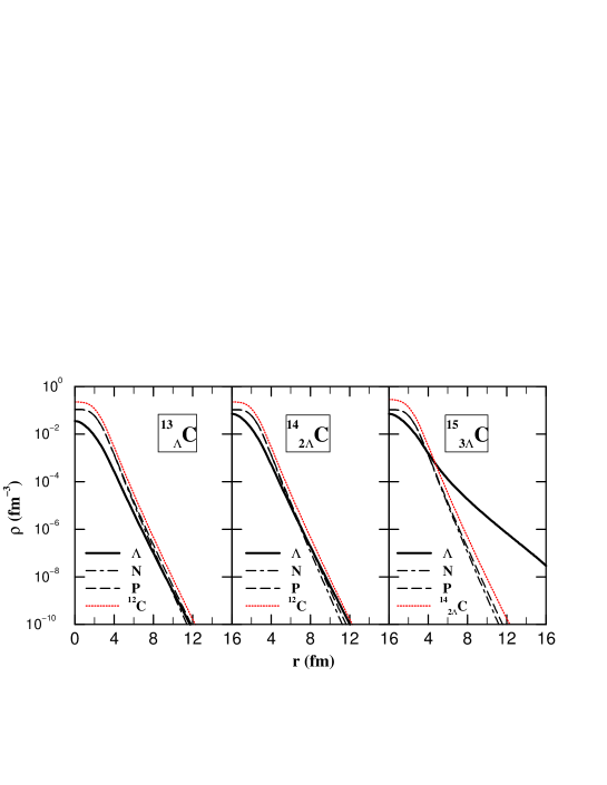
Figure 43: Density distributions for $\Lambda$ (solid), neutron (dot-dashed), proton (long-dashed) and corresponding core (dotted) in ${}^{13}_{\Lambda}$C, ${}^{14}_{2\Lambda}$C and ${}^{15}_{3\Lambda}$C in logarithmic scales. Taken from Ref. [193].

Apart from neutron halos in hyper nuclei, as $\Lambda$ hyperon is less bound than the corresponding nucleon in nuclei, it is worth investigating the existence of hyperon halos. In Ref. [194], a lambda halo was tentatively suggested in a RMF plus BCS model. However, the normal BCS method will have unphysical solution by involving baryon gas [42], such prediction needs further study. Therefore hyper carbon isotopes are studied by RCHB theory in Ref. [193]. In Fig. 43, the baryon density distributions in logarithmic scales versus the radius $r$ in hyper nuclei ${}^{13}_{\Lambda}$C, ${}^{14}_{2\Lambda}$C and ${}^{15}_{3\Lambda}$C are presented, where the solid, dot-dashed, long-dashed and dotted lines represent density distributions for the lambda, neutron, proton, and corresponding core, respectively. It can be seen that up to two $\Lambda$ hyperons added to the core ¹²C, the nucleon density distributions remain the same and hyperon density distributions at the tail are comparable with those of the nucleons. An intriguing phenomenon appears in ${}^{15}_{3\Lambda}$C where the hyperon density distribution has a long tail extended far outside of its core ${}^{14}_{2\Lambda}$C (denoted by dotted line), as shown in the right panel of Fig. 43. This is a signature of hyperon halo. It is due to the weakly bound state $1p_{3/2}^{\Lambda}$ in ${}^{15}_{3\Lambda}$C which has a small hyperon separation energy and a density distribution with long tail.

5 Magic numbers for superheavy nuclei

One of the fundamental and persistent questions in nuclear science is the exploration for the limits of charge and mass that a nucleus can attain and the creation of nuclei with masses and charges much larger than those we are familiar with, i.e., superheavy nuclei. The properties of superheavy nuclei are important to understand not only the nuclear structure, but also the structure of the stars and the evolution of the universe. However, after lots of efforts for both higher luminosities and better detection efficiencies as well as the impressive progresses on the synthesis of superheavy nuclei, the borders of the upper-right corner in the nuclear chart still remain unknown.

Due to fission resulting from the balance of the attractive nuclear surface tension and the repulsive Coulomb force, the superheavy nuclei cannot exist in the classical charged liquid-drop model. The stability of superheavy nuclei is mainly determined by shell effects. At the magic proton or neutron numbers 2, 8, 20, 28, 50, and 82, as well as N=126 for neutrons, nuclei have higher stability and abundance compared with their neighbors. Particularly, the highest stability is observed in the case of the doubly magic nuclei. Amongst other special properties, the doubly magic nuclei are spherical. A semblance of the same would work also for superheavy nuclei, if there were magic numbers in this region. Consequently, these nuclei will be guarded against a faster decay by fission and have more opportunities to be bound. Therefore, it is important to find out the regions in the ($Z$, $N$) plane where the shell effects are strong and the long lifetimes of the superheavy nuclei can be expected.

The pioneering works on the superheavy elements are a series of macro-microscopic nuclear shell model calculations performed over more than 30 years to determine nuclear masses and energy surfaces, which suggested the existence of a group of relatively stable nuclei separated in neutron and proton numbers from the known heavy elements by a higher instability when approaching the closed spherical shells Z=114 and N=184 [195, 196, 197, 198]. This group of nuclei become to be known as the island of superheavy elements and the verification of their existence is one of the most challenging topics in world-wide heavy ion research facility.

Experimentally, however, although the superheavy elements up to $Z$=116 are synthesized or claimed to be synthesized [199, 200, 201, 202, 203, 204, 205, 206, 207, 208, 209, 210, 211, 212] by different heavy ion reaction types including the cold, warm and hot fusion reactions, they are not examples of the originally thought island of superheavy elements yet.

There is no consensus among different theories with regard to the center of the island of superheavy nuclei. Based upon phenomenological models such as finite-range droplet model (FRDM), the shell closures were predicted at $Z$=114 and $N$=184 [213]. Additionally, the FRDM also predicts larger shell gaps at $Z$=104, 106, 108, 110 and at $N$=162, 164 [213]. In Nilsson-Strutinsky scheme, a similar pattern of deformed nuclei have been predicted about $Z$=108 and $N$=162 as in FRDM [214, 215]. However, the main obstacle is the question whether the macroscopic approaches which apply to the region of $\beta$-stability line can be extrapolated to the superheavy nuclei. Recently, microscopic calculations [216, 217, 218, 219, 220, 221, 87, 222, 223, 224, 225, 226] are also attempted in describing the superheavy nuclei. In the framework of RHB theory, calculations with a finite-range pairing force of Gogny interaction D1 and effective interaction NLSH show that $Z$=114 and $N$=160, $N$=166, $N$=184 exhibit stability compared to their neighbors and indications for a doubly magic character at $Z$=106 and $N$=160 are also observed [217]. The Skyrme Hartree-Fock (SHF) method with interactions SkP and SLy7 predicts magic numbers at $Z$=126 and $N$=184, and also predicts the increased stability due to the deformed shell effects at $N$ = 162 [218]. Considering non-relativistic SHF effective interactions SkM*, SkP, SLy6, SkI1, SkI3, SkI4 and relativistic mean field (RMF) effective interactions PL-40, NLSH, NL-Z, TM1, the doubly magic spherical nuclei ₁₈₄114, ₁₇₂120 and ₁₈₄126 based on two-nucleon gaps $\delta_{2p}$ and $\delta_{2n}$ are given [219]. The uncertainty on the magic numbers lies in the uncertain strength of the spin-orbit coupling in non-relativistic approaches or the effective interactions in relativistic models. The prediction of magic numbers in superheavy nuclei remains a challenge for the nuclear models, which have to be rigorously tested by a wide variety of nuclear properties throughout the periodic table.

As the RCHB formalism allows for the proper description of the coupling between the bound states and the continuum by the pairing force and has shown a remarkable success in the description of nuclei with unusual $N/Z$ ratio  [36, 43, 42, 46, 44], it is suitable to apply the RCHB theory for superheavy nuclei. In principle, only a calculation in a large multidimensional deformation space can definitively decide the appropriate ground-state shape. However, as the traditional superheavy nuclei are expected to be spherical and are located on the nuclear chart around a spherical doubly magic nucleus next to ${}^{208}_{126}$Pb, the RCHB theory with the assumption of spherical shape can be applied for the search. Therefore here we will mainly focus on the magic numbers in spherical superheavy nuclei. Some crucial observables in searching shell closures and magic numbers are taken into account, including two-nucleon separation energies, two-nucleon gaps, the shell correction energies, as well as the pairing energies and the effective pairing gaps. At the end of this section, a brief discussion on the stability of the doubly spherical nuclei against deformation and the main progress on the investigation of the deformed superheavy nuclei will be given, as well as the $\alpha-$ decay half-lives of superheavy nuclei.

5.1 Two nucleon separation energies

Traditionally, the magic nuclei are characterized by higher stability than their neighboring ones and the magic numbers can be revealed by the differences of the binding energy, i.e. the one- or two-nucleon separation energies [16]. Therefore, the nucleon separation energies are good starting points to investigate the magic numbers in superheavy region. Due to the absence of odd-even effects, the two-nucleon separation energy $S_{2p}$ ($S_{2n}$) is better to quantify shell effects than the single-nucleon separation energy $S_{p}$ ($S_{n}$). For an isotonic (isotopic) chain, the $S_{2p}$ ($S_{2n}$) decrease with the proton (neutron) number and its sudden jump indicates the occurrence of a proton (neutron) magic number.

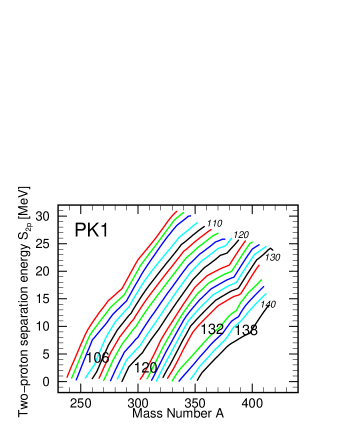
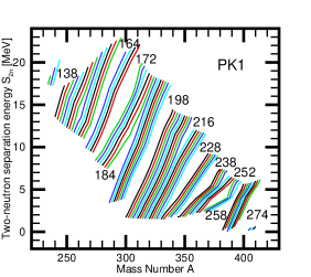
Figure 44: The two-proton(left panel) and two-neutron (right panel) separation energies, $S_{2p}$ and $S_{2n}$, as a function of mass number $A$ obtained by RCHB calculation with PK1 effective interaction. Taken from Ref. [48].

In Ref. [48], the two-proton and two-neutron separation energies have been investigated in the superheavy region with proton number $Z$ ranging from 100 to 140 and neutron number $N$ from $(Z+30)$ to $(2Z+32)$ by the RCHB theory with NL1, NL3, NLSH, TM1, TW99, DD-ME1, PK1 and PK1R. As an example, the results with PK1 are shown as a function of mass number $A$ in Fig. 44. For the proton in left panel, the large gaps appear at $Z=106,120,132,138$, while the usual $Z$=114 does not appear. Furthermore, all the gaps are strongly neutron dependent. On the neutron side in right panel, the relatively larger gaps can be seen at $N$=138, 172, 184, 198, 228, 238, 252, 258, and 274, and also the size and the shape of the gaps differ notably.

From similar investigations with other effective interactions [48], it is found that the magic proton numbers $Z$=120, 132, and 138 are common while $Z$=106 is observed only for NL3, NLSH, TW99, PK1, and PK1R. Furthermore the gaps do not exist for all isotopes. On the neutron side, $S_{2n}$ show distinguishable gaps at $N$=138, 172, 184, 198, 228, 238, 252, 258, and 274 with all the effective interactions. Apart from these, there are also other gaps which appear only for some effective interactions, e.g., $N$ = 164 for NLSH, TW99, DD-ME1, PK1 and PK1R, and $N$ = 216 for NLSH, TW99, PK1, and PK1R. For the magic numbers marked either by the common gaps or the interaction-dependent gaps, the shell quenching phenomena, i.e., the gaps at $N$=184, 198 (NL1), 216 (NLSH, TW99, PK1, and PK1R), 228 (NL1, NL3, NLSH, TM1, PK1, and PK1R), 238, 252, and 258 (NLSH, TM1, PK1, and PK1R) appear only for certain $Z$, are observed.

5.2 Two-nucleon shell gaps

The changes of the two-nucleon separation energies can be quantified by the second difference of the binding energies, i.e., the two-nucleon shell gaps:

$$\delta_{2p}(N,Z) = S_{2p}(N,Z)-S_{2p}(N,Z+2)=2E_{B}(N,Z)-E_{B}(N,Z+2)-E_{B}(N,Z-2)$$ (126)

$$\delta_{2n}(N,Z) = S_{2n}(N,Z)-S_{2n}(N+2,Z)=2E_{B}(N,Z)-E_{B}(N+2,Z)-E_{B}(N-2,Z).$$

A pronounced peak of the two-nucleon shell gaps corresponds to a drastic change of the two-nucleon separation energies and indicates the shell closure [227]. So far, the two-nucleon shell gaps have been extensively used to be an indicator for the magic number [219, 221] and to analyze the shell quenching phenomenon [228].

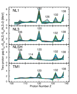
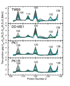
Figure 45: The two-proton shell gaps, $\delta_{2p}$, as a function of proton number obtained by RCHB calculation with effective interactions NL1, NL3, NLSH, TM1, TW-99, DD-ME1, PK1, and PK1R, respectively. Taken from Ref. [48].

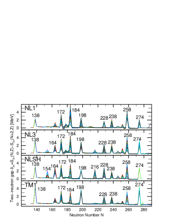
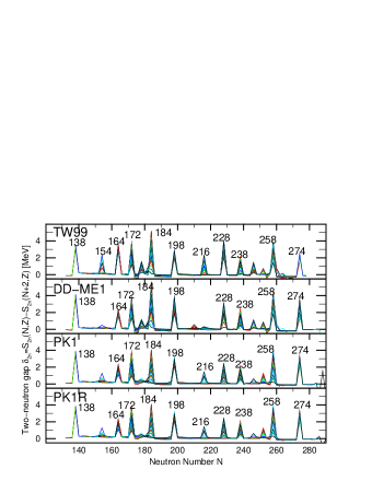
Figure 46: The two-neutron shell gaps, $\delta_{2n}$, as a function of neutron number obtained by RCHB calculation with effective interactions NL1, NL3, NLSH, TM1, TW-99, DD-ME1, PK1, and PK1R, respectively. Taken from Ref. [48].

The two-proton gaps $\delta_{2p}$ from the RCHB calculations for even-even nuclei with $Z$=102 - 138 as a function of $Z$ are shown in Fig. 45. The two-proton gaps $\delta_{2p}$ with the same $N$ are connected as a curve. A peak at certain $Z$ in the curve suggests the existence of magic proton number. The sharpness of the peaks represent the goodness of the magic numbers while the quenching effects are associated with the bundle of the curves at the certain $Z$. The size of the gaps of two-proton separation energies $S_{2p}$ in Fig. 45 correspond to the magnitude of the peaks of two-proton gaps $\delta_{2p}$ in Fig. 45. It is observed that common magic proton numbers $Z$=120, 132, and 138 exist for all the effective interactions while $Z$=106 is observed only for NL3, NLSH, TW99, DD-ME1, PK1, and PK1R. Furthermore, the peak at $Z$=114 for NLSH and TW99 and the peak at $Z$=126 for NL1 are also observed, though they are not so obvious as that at $Z$=120.

Similar figure for two-neutron gaps $\delta_{2n}$ are shown in Fig. 46. There are interaction-independent peaks of two-neutron gaps $\delta_{2n}$ at $N$=138, 172, 184, 198, 228, 238, 258, and 274 which are consistent with the conclusion from the two-neutron separation energies $S_{2n}$ . Moreover, small peaks are also observed for $N$=154 (NLSH and TW99), $N$=164 (NL3, NLSH, TW99, DD-ME1, PK1, and PK1R), and $N$=216 (NLSH, TW99, PK1, and PK1R).

5.3 Shell correction energies

The shell correction energy, representing the overall behavior of the single-particle spectra, is another suitable observable to identify the shell closure. This quantity, which is derived from the single-particle spectra by the Strutinsky procedure [229], is defined as the difference between the total single-particle energy $E$ and the smooth single-particle energy $\bar{E}$:

$$E_{shell}=E-\bar{E}=\sum\limits_{i=1}^{N(Z)}{e_{i}}-2\int\limits_{-\infty}^{\bar{\lambda}}{e\bar{g}(e)de},$$ (127)

where $N(Z)$ is the particle number, $e_{i}$ is the single-particle energy, $\bar{\lambda}$ is the smoothed Fermi level determined by the particle number equation $N(Z)=2\int\limits_{-\infty}^{\bar{\lambda}}{\bar{g}(e)de}$, and $\bar{g}(e)$ is the smoothed level density

$$\bar{g}(e)=\dfrac{1}{\gamma}\int\limits_{-\infty}^{\infty}{\left(\sum\limits_{i=1}^{\infty}{\delta(e^{\prime}-e_{i})}\right)f(\frac{e^{\prime}-e}{\gamma})de^{\prime}}=\dfrac{1}{\gamma}\sum\limits_{i=1}^{\infty}{f(\dfrac{e_{i}-e}{\gamma})},$$ (128)

with the smoothing range $\gamma$ , the folding function $f(x)=\dfrac{1}{\sqrt{\pi}}e^{-x^{2}}P(x)$, and $P(x)$ the associated Laguerre polynomial $L_{s}^{1/2}(x^{2})$. The shell correction energy provides an indicator about the deviation in the level structure of nuclei away from uniformly distributed ones. A large negative shell correction energy corresponds to shell closure at certain nucleon number.

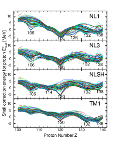
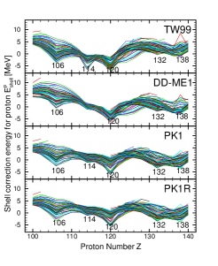
Figure 47: The shell correction energies for proton, $E_{shell}^{p}$, as a function of proton number obtained by RCHB calculation with effective interactions NL1, NL3, NLSH, TM1, TW-99, DD-ME1, PK1 and PK1R, respectively. Taken from Ref. [48].

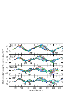
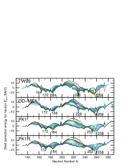
Figure 48: The shell correction energies for neutron, $E_{shell}^{n}$, as a function of neutron number obtained by RCHB calculation with effective interactions NL1, NL3, NLSH, TM1, TW-99, DD-ME1, PK1 and PK1R, respectively. Taken from Ref. [48].

With the proton single-particle spectra in canonical basis from the RCHB calculations, the shell correction energies $E_{shell}^{p}$ for even-even nuclei with $Z$ ranging from 100 to 140 are shown as a function of $Z$ in Fig. 47. The nuclei with the same $N$ are connected as a curve. A deep valley at certain $Z$ on a curve hints the shell closure. The valleys at $Z$=120, 132, and 138 are conspicuous for all the effective interactions. Possible shell closure at $Z$=106 for NL1, NL3, NLSH, TW99, DD-ME1, PK1, and PK1R, at $Z$=114 for NLSH, TW99, PK1, and PK1R, and at $Z$=126 for NL1 are also observed. The shell closure from the shell correction energies for proton $E_{shell}^{p}$ are consistent with the peaks of the two-proton gaps $\delta_{2p}$, though the magnitude of magicity slightly differs. Similar to the two-proton gaps $\delta_{2p}$, the spread of the valleys of the shell correction energies for proton $E_{shell}^{p}$ indicates the quenching of the magic number. In view of the shell correction energies for proton $E_{shell}^{p}$, the quenching phenomena of magic proton numbers in RCHB calculation are universal. These facts suggest that the magic proton numbers depend also on neutron number $N$.

The corresponding shell correction energies for neutron $E_{shell}^{n}$ for even-even nuclei with $N$=130 - 312 are demonstrated as a function of $N$ in Fig. 48. As the neutron numbers extend from $N$=130 to $N$=290, the valleys for shell correction energies for neutron $E_{shell}^{n}$ in Fig. 48 are not so obvious as those for shell correction energies for proton $E_{shell}^{p}$ in Fig. 47. However, similar conclusions as the two-neutron separation energies $S_{2n}$ and the two-neutron gaps $\delta_{2n}$ for magic neutron numbers can also be drawn. Similar calculation has also been done in Ref. [230] with SHF and RMF.

The first valley locates in $N$=184 for all the effective interactions and involves $N$=172 (NL3, NLSH, TM1, TW99, DD-ME1, PK1, and PK1R), even $N$=164 (NLSH and TW99). And the other valley is the mixture of the valleys at $N$=228 (TW99 and DD-ME1), $N$=252 (NLSH, TM1, PK1, and PK1R) and $N$=258. These fine structures suggest the smearing of magic neutron numbers. Based on the shell correction energies, the shell closures are smeared compared with those from the two-nucleon separation energies $S_{2p}$ and $S_{2n}$ and the two-nucleon gaps $\delta_{2p}$ and $\delta_{2n}$. However, it is found in Ref. [48] that the magic numbers at $Z$=120, 132, and 138 are common but strongly quenched, the shell closures near $N$=172 and $N$=184, and $N$=228, $N$=252, and $N$=258 are blurred. The other magic numbers from the shell correction energies, such as $Z$=106, 114, and 126, appear only for some effective interactions.

In the usual Hartree or HF mean field level, as the nonphysical particle continuum are involved, much efforts have been made to avoid the divergence of single particle energy density around the threshold [231, 232, 233, 234]. Based on the Green’s-function approach to the level density, a method of calculating shell corrections has been adopted within the SHF and RMF theories to a large-scale survey of spherical shell energies throughout the whole landscape of conceivable superheavy nuclei [230]. From SHF with SkP, SLy6, SkI3 and SkI4 and RMF with NL3 and NL-Z2, the total shell correction energies $E_{shell}$ for spherical superheavy nuclei around the expected island of stability around $Z$ = 120 and $N$ = 180 are given in Fig. 49. Instead of narrow stripes of large $E_{shell}$ localized around magic numbers for normal nuclei, a wide area of shell stabilization is found to spreads over all shell closures predicted. In other words, the predicted magic shells for superheavy nuclei are much mellowed, which are consistent with the results from RCHB theory. The disappearance of a familiar pattern of magic numbers and the appearance of broad valleys of shell stability are due to the rather large single-particle level density and the appearance of many low $j$ shells around the Fermi level [230].

Figure 49: Total shell correction energies, calculated from SHF with SkP, SLy6, SkI3 and SkI4 and RMF with NL3 and NL-Z2, for spherical even-even superheavy nuclei around the expected island of stability around $Z$ = 120 and $N$ = 180. The thick solid lines denote two-particle drip lines. Black squares mark nuclei calculated to be stable with respect to $\beta$ decay. White color indicates nuclei with positive shell corrections, black color denotes nuclei with $E_{shell}$ beyond -12 MeV. Taken from Ref. [235].

5.4 Magic numbers and deformations

5.4.1 Magic numbers for spherical superheavy nuclei

After the detailed analysis of the two-nucleon separation energies, $S_{2p}$ and $S_{2n}$, the two-nucleon shell gaps, $\delta_{2p}$ and $\delta_{2n}$, the shell correction energies, $E_{shell}^{p}$ and $E_{shell}^{n}$, as well as the pairing effects, the magic numbers for superheavy nuclei in the RCHB theory are found to be [48]: $Z=120,132,138$ for proton and $N=172,184,198,228,238,258$ for neutron. As many theoretical methods have been adopted to probe the superheavy magic numbers and there is no consensus among them with regard to the center of the island of superheavy nuclei. It is interesting to briefly review the up-to-date studies of the superheavy magic numbers including the present one:

• $Z$=106: As we have seen, this shell closure is strongly supported by the effective forces NL3, NLSH, TW-99, PK1, and PK1R, partially by NL1 and DD-ME1, but not at all by TM1. We also noted that the shell closure at $Z$=106 depends sensitively on the neutron number and is visible only around $N$ $\sim$ 154 and $\sim$ 218, while the later can only be clearly seen in the results calculated with TW-99 and NLSH. The RHB calculations with the effective force NLSH and the Gogny interaction D1 for the pairing correlation predicts a doubly magic character at $Z$=106 and $N$=160 [217]. In addition, the shell closures at $Z$=104, 106, 108, and 110 and $N$=162, and 164 which correspond to prolate deformations are predicted by the FRDM [213] and the deformed shell closure occurs at $Z$=108 in Nilsson-Strutinsky scheme [214, 215].

• $Z$=114: The shell closures are predicted at $Z$=114 and $N$=184 in the phenomenological shell models [197, 198, 214, 213]. However, as we have noted, in the RCHB theory the magicity of $Z$=114 is not at all obvious, in agreement with other RMF investigations [219, 217, 236, 22, 237]. By adopting a new effective interaction NL-RA1, the nucleus ${}^{298}_{184}114$ is predicted to be the next spherical doubly magic nucleus in a RMF plus BCS calculation [238]. Within the SHF approach, only SkI4 prefers the doubly magic nucleus at $Z$=114 and $N$=184, which is not supported by other Skryme forces such as SkM*, SkP, SkI1, SkI3, SLy6, and SLy7 [219, 221].

• $Z$=120: The shell closure at $Z$=120 is strongly supported in the RCHB calculations. The doubly magic characteristic of ${}^{292}_{172}120$ has been addressed within the RMF theory [219, 221, 238, 234] as well as the effective field theory [237]. Most Skyrme HF investigations also suggest that this nucleus is doubly magic except for SkP [219, 221]. Due to the strong shell quenching effect in the $Z$=120 isotopic chain, other doubly magic candidates with $N$=184, 198, 228, 238, 252, 258, and 274 are interaction-dependent and need to be investigated in more detail.

• $Z$=126: Several Skyrme HF investigations with the effective interactions such as SkP, SkM*, SLy6 and SLy7 predict doubly magic system at $Z$=126 and $N$=184 [218, 219, 221]. However, this conclusion is not supported by the RMF calculations although $N$=184 might be a neutron magic number.

• $Z$=132 and 138: Little attention has been paid to the possible proton shell closures at $Z>130$ due to their large Coulomb repulsive potentials. However, the shell closures at $Z$=132 with $N\sim$ 210-240, and at $Z$=138 with $N\sim$ 180-200 and $N\sim$ 258 appear in most relativistic and non relativistic mean field models [219, 48], .

Normally the magic numbers correspond to the large energy gaps between the single particle levels and the doubly magic nuclei are those with protons and neutrons filled up to the gap. It is therefore interesting to study the single-particle level structure in these doubly magic nuclei, or vice versa.

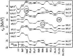
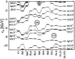
Figure 50: Spherical single particle spectra in ${}^{292}_{172}$120 for protons (left) and neutrons in various mean-field calculations as indicated. Taken from Ref. [221].

As examples, the spherical single particle spectra in ²⁹²120 for protons (left) and neutrons in various mean-field calculations are given in Fig. 50 [221]. The occurrence of the shell closure at $Z=120$ depends on the amplitude of the spin-orbit splitting of the 3p states above the Fermi level and the 2f levels below the Fermi energy. It has also been pointed out that the shell closures may be coupled to the density profiles (and vice versa) based on the systematic analysis of density distribution of superheavy nuclei. For ²⁹²120, a significant central depression or central semibubble is obtained in the spherical case [221, 239]. Recently, the influence of the central depression in the density distribution of spherical superheavy nuclei on the shell structure is studied in some detail within the RMF theory [240]. It is found that a large depression leads to the shell gaps at the proton $Z$ = 120 and neutron $N$ = 172 numbers, whereas a flatter density distribution favors $N$ = 184 and leads to the appearance of a $Z$ = 126 shell gap and to the decrease of the size of the $Z$ = 120 shell gap. On the other side, the deformation effect has been found to be significant in the calculation of the density distribution in this nucleus, namely only a weak central depression in the deformed case for ²⁹²120 compared to the predicted semibubble at the spherical shape [241, 240].

5.4.2 Stability of the doubly magic superheavy nuclei against deformation

The magic numbers discussed above are mainly based on the assumption of spherical geometrical configuration. However, such assumption is not always true for superheavy nuclei [213, 214, 215, 242]. It is worthwhile to investigate the potential energy surfaces to see the validity of spherical configuration.

In Fig. 51, the potential energy surfaces for ²⁹²120, ³⁰⁴120, ³¹⁸120, ³⁴⁸120, ³⁵⁸120, and ³⁷⁸120 (solid lines) obtained from constrained RMF calculations with the pairing correlations treated by BCS approximations are displayed. Although these nuclei have the same proton number, their potential energy surfaces are quite different from each other as shown in Fig. 51. For nuclei ²⁹²120, ³⁰⁴120 and ³⁷⁸120, there is an obvious local minimum with the spherical configuration $\beta_{2}\sim 0$, while another local minimum with large deformation $\beta_{2}\sim 0.6$ can be also clearly seen. For ³¹⁸120, the spherical local minimum is very shallow, and for ³⁴⁸120 and ³⁵⁸120, the spherical minimum is hardly seen and a local minimum with $\beta_{2}\sim 0.25$ appears instead. There are also local minimum around $\beta_{2}\sim-0.4$ with oblate deformation. In addition to the local minima discussed above, we would like to make a few remarks on the absolute minima for these nuclei. For ²⁹²120 and ³⁷⁸120, the two minima with different deformations have almost the same energies, i.e. the so-called “shape coexistence” may exist. In particular, the spherical minimum is indeed the absolute minimum for ²⁹²120 ($E_{B}=$ -2064.3 MeV with $\beta_{2}\sim 0$ vs. $E_{B}=$ -2063.6 MeV with $\beta_{2}\sim 0.6$), while the ground state of ³⁷⁸120 is quite delicate with $E_{B}=$ -2398.7 MeV for $\beta_{2}\sim 0$ and $E_{B}=$ -2398.7 MeV for $\beta_{2}\sim 0.6$. For ³⁰⁴120, the absolute minimum at $\beta_{2}\sim 0.6$ is much deeper ($\sim$ 5.5 MeV) than the spherical configuration. In addition for ³⁴⁸120, the absolute minimum lies at $\beta_{2}\sim 0.2$, and it is a well-deformed nucleus according to the present calculation. From the RCHB and the constrained RMF+BCS calculations, it is shown that spherical doubly magic nuclei may exist, e.g., ²⁹²120 and ³⁷⁸120 [48].

The role of shell effects in superheavy nuclei can be also seen in Fig. 51, in which the corresponding macroscopic energy, defined as the difference between the binding energy and the total shell correction energy, $E_{B}-E_{\mathrm{shell}}$, is plotted with dashed lines. It can be seen that without the shell effects, the superheavy nuclei hardly exist. As noted long time ago, the shell effects play an essential role to stabilize the superheavy nuclei against the fission.

Figure 51: The total energy, $E_{B}$, and the equivalent macroscopic energy, $E_{B}-E_{\mathrm{shell}}$, of ^{292,304,318,348,358,378}120 calculated in the constrained RMF theory with effective interaction NL3. Taken from Ref. [48].

Apart from axial symmetric case, the influence of other deformation such as triaxiality and reflection asymmetry deformations has been investigated as well, e.g., see Ref.[23, 226]. Figure 52 presents an example of potential energy surface of the typical actinide nucleus ²⁴⁰Pu, which has often served as a benchmark for mean-field models, obtained with the Skyrme force SLy6. A typical doubled-humped fission barrier is well shown. The inner barrier explores triaxial degrees of freedom, which reduce the axial barrier by about 3 MeV, while the outer barrier explores reflection asymmetric shape [226]. The similar behavior is held for heavier nuclear system [220]. It is also noted that though the further deformation degrees of freedom reduce the fission barriers obviously, they hardly change the energies of mimina. Therefore, the constraint RMF model with axial symmetry remains valid to confirm the spherical configuration of a superheavy nucleus.

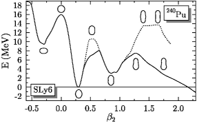
Figure 52: Double-humped fission barrier of the typical actinide nucleus ²⁴⁰Pu. The dotted line denotes an axial and reflection-symmetric calculation, the full line denotes a triaxial (inner barrier) and axial and reflection-asymmetric calculation (outer barrier). The various shapes along the axial paths are indicated by the contours of the total density at $r_{0}=0.07$ fm^-3. Taken from Ref.[226]

5.5 Alpha decay and the half-lives

The preferred decay mode of shell stabilized superheavy nuclei is $\alpha$ decay. A key quantity for $\alpha$ decay, the $Q_{\alpha}$ value is defined as

$$Q_{\alpha}(N,Z)=E(N,Z)-E(N-2,Z-2)-E(2,2),$$ (129)

which is the energy of the $\alpha$-particles emitted by radioactive heavy and superheavy nuclei. It is interesting to compare the $Q_{\alpha}$ data of the discovered superheavy nuclei with predictions from mean-field models. Such works have been done in various of mean field framework, e.g. Refs. [222, 223, 224, 225, 23, 243]. In the recent experiments designed to synthesize the element 115 in the ²⁴³Am+⁴⁸Ca reaction at Dubna in Russia, three similar decay chains consisting of five consecutive $\alpha$-decays, and another different decay chain of four consecutive $\alpha$-decays are observed, and the decay properties of these synthesized nuclei are claimed to be consistent with consecutive $\alpha$-decays originating from the parent isotopes of the new element 115, ${}^{288}115$ and ${}^{287}115$, respectively [212]. The deformed RMF+BCS calculation with a density-independent delta-function interaction in the pairing channel and the effective interaction TMA is made to study these newly synthesized superheavy nuclei ${}^{288}115$, ${}^{287}115$, and their $\alpha$-decay daughter nuclei [225]. The calculated $\alpha$-decay energies and half-lives agree well with the experimental values and with those of the macroscopic-microscopic FRDM+FY and YPE+WS models.

For an area of enhanced stability, the $\alpha$-decay half-lives are expected to be longer than its neighbors. The half-lives of $\alpha$-decay can be obtained with $Q_{\alpha}$ value by phenomenological Viola and Seaborg systematics [244]:

$$log_{10}T_{\alpha}=(1.66175Z-8.5166)Q_{\alpha}^{-1/2}-(0.20228Z+33.9069)$$ (130)

where $Z$ is the proton number of the parent nucleus, $T_{\alpha}$ in second and the parameters taken from Ref. [245]. It should be noted that Eq. (130) is based on the WKB approximation, and provides only a rather crude estimation of $T_{\alpha}$ since it disregards many structure effects such as deformation, and configuration changes, etc.

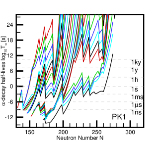
Figure 53: The $\alpha$-decay half-lives $T_{\alpha}$ as a function of neutron number obtained by RCHB calculation with PK1 effective interaction. Taken from Ref. [48].

In Fig. 53, the half-lives $T_{\alpha}$ from the RCHB calculation in logarithm scale are plotted as a function of neutron number $N$ with the effective interaction PK1. The half-lives corresponding to 1 ns, 1 $\mu$s, 1 ms, 1 s, 1 h, 1 y, and 1 ky are marked by the dashed lines. Each curve in this figure corresponds to an isotopic chain in the region with $Z$ ranging from 102 to 140. In Fig. 53, the half-lives $log_{10}T_{\alpha}$ increase with $N$. The jumps of the curves correspond to magic proton numbers $Z$=106, 120, 132, and 138, which depend on the effective interactions. The peaks of each curve correspond to magic neutron numbers, i.e., $N$=172, 184, 228, 238 and 258. It can be seen that the magic numbers suggested by two-neutron separation energies $S_{2n}$(two-neutron gaps $\delta_{2n}$) or two-proton separation energies $S_{2p}$ (two-proton gaps $\delta_{2p}$) can also be found here. It should be noted that the half-lives $T_{\alpha}$ shown here are obtained from the spherical RCHB calcualtions. In fact, both the pairing correlation and deformation are essential to reproduce the experiment $Q_{\alpha}$ values [222, 224, 246]. Calculations along this line are necessary.

6 Summary and perspectives

This article has been concerned with the relativistic description of the exotic nuclei particularly with the Relativistic Continuum Hartree-Bogoliubov (RCHB) theory and its applications. The last two decades have witnessed the development of the relativistic mean field (RMF) theory and its successful application in nuclear physics. At the very beginning, the question on the clear signal of relativistic effects in atomic nuclei has puzzled us for quite a long time. Now after lots of efforts, it become evident that there are at least the following points which do favor the relativistic description of nuclei:

• One may say that the kinetic energy of a nucleon moving in an nucleus is much smaller than its mass. However, as far as the mass is concerned, we have to remember that the mass of a nucleus is smaller than the sum of the mass of its consistent nucleons, which is naturally obtained in a relativistic model. Furthermore there are always a large scalar and a large vector potentials which are both comparable to the mass of the nucleons in nucleus.

• Relativistically the spin-orbit potential comes out naturally. Furthermore the long existing problems on the origin of pseudo-spin symmetry were solved. A very well developed spin symmetry in single anti-neutron and single anti-proton spectra is found. This spin symmetry in anti-particle spectra and the pseudo-spin symmetry in particle spectra have the same origin.

• In the framework of the relativistic approach, the nucleons interact via the exchanges of mesons and photons. From this point of view, the relativistic approach is more microscopic and fundamental in the sense of describing the nuclear system at the meson level.

• In practice, it turns out that the RMF theory can reproduce better the nuclear saturation properties (the Coester line) in nuclear matter and the isotopic shifts in the Pb-region, and is more reliable for nuclei far away from the line of $\beta$-stability.

Altogether the relativistic mean field theory is a reliable and effective model for nuclear structure. Therefore, with the fast progress in producing the exotic nuclei, it is natural to describe the exotic nuclei based on the RMF theory.

The formalism, the numerical solutions and the effective interactions for the RMF theory as well as its application for nuclear matter and neutron stars are presented in Section 2. The numerical solutions of the Dirac equation for spherical nuclei, particularly on the Woods-Saxon basis, are discussed in detail. The new effective interactions with nonlinear self-coupling meson fields and density dependent meson-nucleon couplings, and their influences on properties of nuclear matter and neutron stars are also discussed.

Pairing correlation plays important roles in open shell nuclei. The conventional BCS method can be combined easily with the RMF theory, but it is not justified for exotic nuclei because it could not include properly the contribution of continuum states. The formalism and related discussions of the RCHB theory, in which the coupling between the bound states and continuum could be included self-consistently, are given in Section 3. Discussion on the continuum states, the resonant BCS method and several methods for obtaining single particle resonant states are briefly reviewed.

The study of exotic nuclei has attracted world wide attention due to their large $N/Z$ ratios (isospin) and interesting properties such as halo and skin. In Section 4 we reviewed the application of the RCHB theory to exotic nuclei, the binding energies, particle separation energies, the radii and cross sections, the single particle levels, shell structure, the restoration of the pseudo-spin symmetry, the halo and giant halo, and halos in hyper nuclei, etc. For examples, (1) the Li isotopes were investigated and the halo phenomenon in ¹¹Li was found to be the result of the scattering of particle pairs into continua; (2) the giant halos were predicted in Zr, Ca and even lighter nuclei when neutron drip line is approached based on the analysis of two neutron separation energies, single particle energy levels, the orbital occupation, the contribution of continuum and nucleon density distribution. These predictions are supported to some extent by the recent experimental information; (3) exotic phenomena in hyper-nuclei were also studied; etc.

The RCHB theory has been applied to study superheavy nuclei which is reviewed in Section 5. The possible doubly magic superheavy nuclei have been searched within the RCHB theory using a variant of the effective interactions. Base on the detailed analysis on the two-nucleon separation energies $S_{2p}$ and $S_{2n}$, two-nucleon shell gaps $\delta_{2p}$ and $\delta_{2n}$, the shell correction energies $E_{shell}^{p}$ and $E_{shell}^{n}$, as well as the pairing energies $E_{pair}^{p}$ and $E_{pair}^{n}$, the effective pairing gaps $\Delta_{p}$ and $\Delta_{n}$, the proton and neutron shell closures have been predicted by using the RCHB theory with the effective interactions NL1, NL3, NLSH, TM1, TW-99, DD-ME1, PK1 and PK1R. Proton numbers $Z$=120, 132, and 138 and neutron numbers $N$=172, 184, 198, 228, 238, and 258 are supported by all effective interactions to be magic. The deformation-constrained RMF calculations have been done for these doubly magic nuclei candidates and discussions on the deformation of these nuclei are also presented.

Among many perspectives of the application of the RMF and the RCHB theories, we mention briefly the following:

1. Attempts have been made by extending the present RCHB theory for the axially deformed nuclei. Although the coupled Dirac equations and Hartree-Bogoliubov equations with fixed pairing potentials have been solved in coordinate space, the simultaneous self-consistent solution of axially deformed RCHB equations is proved to be very difficult [247]. Therefore the Woods-Saxon basis has been suggested to solving the RMF theory in order to generalize it to study exotic nuclei by solving either the Schrödinger equation or the Dirac equation [73]. It combines the advantages of the efficiencies in harmonic oscillator basis and the appropriateness for exotic nuclei in coordinate space. For spherical case, the Woods-Saxon basis has been proved to be very successful [73]. The development of deformed RCHB in the Woods-Saxon basis is in progress.

2. The Shell-model-Like APproach (SLAP) method has been suggested to treat pairing correlation in RMF theory [248]. With the single particle bound states from the RMF calculation and resonant states obtained from RMF theory combined with the Analytic Continuation of Coupling Constant (ACCC) method [110, 111] or the phase shift scattering method [41, 117], the SLAP for the pairing can also be used to describe exotic nuclei as well.

3. Since the pion does not contribute in the Hartree level, we did not mention its contribution throughout the paper. However, if the Fock term is considered, one must include pion in the Lagrangian. This would bring out some complication in solving the equations as well as new and interesting physics.

4. Many symmetries have been broken in the mean field theory. Restoration of some symmetries could be achieved by making projections or corrections. The microscopic center of mass correction for the broken translation invariance in the RMF model has been discussed [51]. The single particle states of a deformed mean field do not have good total angular momentum, so is the total intrinsic wave function of the deformed nucleus. Thus one must project out a state with good total angular momentum from the intrinsic wave function. This can be done by the full angular momentum projection method [35] or approximately in a simple way [249]. Recent works on the restoration of rotation symmetry [250, 251] are very interesting. Possible extensions and applications for chiral doublet bands and nuclear isomeric states are expected [252, 253, 254, 255, 256, 257, 258] .

5. In most of the RMF calculations, the no-sea approximation is applied. Therefore the anti-nucleon degrees of freedom are not considered. It would be quite interesting to investigate these degrees of freedom and the polarization of the vacuum as well as abnormal nuclei containing anti-baryons [259, 193, 33, 47, 260].

Acknowledgments

The authors would like to thank their colleagues, collaborators and students, in particular, A. Arima, S. F. Ban, T. S. Chen, J. Dobaczewski, H. Geissel, J. Ginocchio, J. Y. Guo, G. C. Hillhouse, Soojae Im, H. Y. Jia, T. T. S. Kuo, A. Leviatan, J. Li, G. L. Long, H. F. Lü, H. Madokoro, M. Matsuzaki, G. Münzenberg, A. Ozawa, J. Peng, P. Ring, N. Sandulescu, J. P. Sang, G. Shen, W. Q. Shen, K. Sugawara-Tanabe, S. Sugimoto, B. H. Sun, B. X. Sun, Y. Sun, N. Takigawa, I. Tanihata, N. Van Giai, S. J. Wang, R. Wyss, S. Yamaji, S. C. Yang, J. Y. Zeng, H. Q. Zhang, J. Y. Zhang, W. Zhang, S. S. Zhang, E. G. Zhao, who contribute directly or indirectly to the investigations presented here. This work was partly supported by the Major State Basic Research Development Program Under Contract Number G2000077407 and the National Natural Science Foundation of China under Grant No. 10025522, 10435010, 10475003 and 10221003, the Doctoral Program Foundation from the Ministry of Education in China and the Knowledge Innovation Project of Chinese Academy of Sciences under contract No. KJCX2-SW-N02.

References

- [1] C. A. Bertulani, M. S. Hussein, G. Münzengerg, Physics of Radioactive Beams, Nova Science Publishers, Inc., 2001.
- [2] W. L. Zhan, in: Invited lectures at INTERNATIONAL SUMMER SCHOOL ON SUBATOMIC PHYSICS, Beijing, 2004.
- [3] Y. Yano, in: The Fifth Japan-China Joint Nuclear Physics Symposium, Fukuoka, Japan, 2004.
- [4] W. Henning, in: Scientific Opportunities and Challenges — China and the International FAIR Project, Beijing, 2004.
- [5] http://www.phy.anl.gov/ria/ or http://www.nscl.msu.edu/ria/index.php.
- [6] A. C. Mueller, B. M. Sherrill, Ann. Rev. Nucl. Part. Sci. 43 (1993) 529.
- [7] I. Tanihata, Prog. Part. Nucl. Phys. 35 (1995) 505.
- [8] P. G. Hansen, A. S. Jensen, B. Jonson, Ann. Rev. Nucl. Part. Sci. 45 (1995) 591.
- [9] R. F. Casten, B. M. Sherrill, Prog. Part. Nucl. Phys. 45 (2000) S171.
- [10] A. C. Mueller, Prog. Part. Nucl. Phys. 46 (2001) 359.
- [11] B. Jonson, Phys. Rep. 389 (2004) 1.
- [12] A. S. Jensen, K. Riisager, D. V. Fedorov, E. Garrido, Rev. Mod. Phys. 76 (2004) 215.
- [13] I. Tanihata, H. Hamagaki, O. Hashimoto, et al., Phys. Rev. Lett. 55 (1985) 2676.
- [14] A. Ozawa, T. Kobayashi, T. Suzuki, K. Yoshida, I. Tanihata, Phys. Rev. Lett. 84 (2000) 5493.
- [15] M. G. Mayer, J. H. D. Jensen, Elementary Theory of Nuclear Shell Struture, Wiley, New York, 1955.
- [16] A. Bohr, B. R. Mottelson, Nuclear Structure, Vol.I, Benjamin, New York, 1969.
- [17] A. Bohr, B. R. Mottelson, Nuclear Structure, Vol.II, Benjamin, New York, 1975.
- [18] J. D. Walecka, Ann. Phys. (NY) 83 (1974) 491.
- [19] B. D. Serot, J. D. Walecka, The Relativistic Nuclear Many-Body Problem in Advances in Nuclear Physics, edited by J. W. Negele and E. Vogt 16 (1986) 1.
- [20] P.-G. Reinhard, Rep. Prog. Phys. 52 (1989) 439.
- [21] P. Ring, Prog. Part. Nucl. Phys. 37 (1996) 193.
- [22] B. D. Serot, J. D. Walecka, Int. J. Mod. Phys. E6 (1997) 515.
- [23] M. Bender, P.-H. Heenen, P.-G. Reinhard, Rev. Mod. Phys. 75 (2003) 121.
- [24] R. J. Furnstahl, Lect. Notes Phys. 641 (2004) 1, and references therein, arXiv: nucl-th/0307111.
- [25] R. Brockmann, R. Machleidt, Phys. Rev. C42 (1990) 1965.
- [26] R. Brockmann, H. Toki, Phys. Rev. Lett. 68 (1992) 3408.
- [27] M. M. Sharma, G. A. Lalazissis, P. Ring, Phys. Lett. B317 (1993) 9.
- [28] A. Arima, M. Harvery, K. Shimizu, Phys. Lett. B30 (1969) 517.
- [29] K. T. Hecht, A. Adler, Nucl. Phys. A137 (1969) 129.
- [30] J. N. Ginocchio, Phys. Rev. Lett. 78 (1997) 436.
- [31] J. Meng, K. Sugawara-Tanabe, S. Yamaji, P. Ring, A. Arima, Phys. Rev. C58 (1998) R628.
- [32] J. Meng, K. Sugawara-Tanabe, S. Yamaji, A. Arima, Phys. Rev. C59 (1999) 154.
- [33] S. G. Zhou, J. Meng, P. Ring, Phys. Rev. Lett. 91 (2003) 262501.
- [34] A. Bulgac, Report No. FT-194-1980 arXiv: nucl-th/9907088.
- [35] P. Ring, P. Schuck, The nuclear many-body problem, Springer-Verlag, New York, 1980.
- [36] J. Meng, P. Ring, Phys. Rev. Lett. 77 (1996) 3963.
- [37] J. Dobaczewski, H. Flocard, J. Treiner, Nucl. Phys. A422 (1984) 103.
- [38] J. Dobaczewski, W. Nazarewicz, T. R. Werner, et al., Phys. Rev. C53 (1996) 2809.
- [39] M. Grasso, N. Sandulescu, N. Van Giai, R. J. Liotta, Phys. Rev. C 64 (2001) 064321.
- [40] M. Grasso, N. Van Giai, N. Sandulescu, Phys. Lett. B 535 (2002) 103.
- [41] N. Sandulescu, L. S. Geng, H. Toki, G. C. Hillhouse, Phys. Rev. 68 (2003) 054323.
- [42] J. Meng, Nucl. Phys. A635 (1998) 3.
- [43] J. Meng, P. Ring, Phys. Rev. Lett. 80 (1998) 460.
- [44] J. Meng, H. Toki, J. Y. Zeng, S. Q. Zhang, S. G. Zhou, Phys. Rev. C65 (2002) R041302.
- [45] J. Meng, I. Tanihata, S. Yamaji, Phys. Lett. B419 (1998) 1.
- [46] J. Meng, S. G. Zhou, I. Tanihata, Phys. Lett. B532 (2002) 209.
- [47] H. F. Lv, J. Meng, S. Q. Zhang, S. G. Zhou, Euro. Phys. J. 17 (2003) 19.
- [48] W. Zhang, J. Meng, S. Q. Zhang, L. S. Geng, H. Toki, Nucl. Phys. A 753 (2005) 106.
- [49] J. Boguta, A. R. Bodmer, Nucl. Phys. A292 (1977) 413.
- [50] Y. Sugahara, H. Toki, Nucl. Phys. A579 (1994) 557.
- [51] W. H. Long, J. Meng, N. Van Giai, S. G. Zhou, Phys. Rev. C69 (2004) 034319.
- [52] S. Kubis, M. Kutschera, Phys. Lett. B399 (1997) 191.
- [53] H. Shen, Y. Sugahara, H. Toki, Phys. Rev. C55 (1997) 1211.
- [54] F. de Jong, H. Lenske, Phys. Rev. C 57 (1998) 3099.
- [55] F. Hofmann, C. M. Keil, H. Lenske, Phys. Rev. C 64 (2001) 034314.
- [56] Z. Y. Ma, L. Liu, Phys. Rev. C66 (2002) 024321.
- [57] B. Liu, V. Greco, V. Baran, M. Colonna, M. Di Toro, Phys. Rev. C65 (2002) 045201.
- [58] D. P. Menezes, C. Providncia, Phys. Rev. C70 (2004) 058801.
- [59] H. Lenske, C. Fuchs, Phys. Lett. B345 (1995) 355.
- [60] C. Fuchs, H. Lenske, H. H. Wolter, Phys. Rev. C52 (1995) 3043.
- [61] S. Typel, H. H. Wolter, Nucl. Phys. A656 (1999) 331.
- [62] T. Niksic, D. Vretenar, P. Finelli, P. Ring, Phys. Rev. C66 (2002) 024306.
- [63] S. G. Nilsson, Dan. Mat. Pys. Medd. 30 (1955) 1.
- [64] M. Stoitsov, P. Ring, D. Vretenar, G. A. Lalazissis, Phys. Rev. C58 (1998) 2086.
- [65] M. V. Stoitsov, W. Nazarewicz, S. Pittel, Phys. Rev. C58 (1998) 2092.
- [66] S. G. Zhou, J. Meng, S. Yamaji, S. C. Yang, Chin. Phys. Lett. 17 (2000) 717.
- [67] D. A. Varshalovich, A. N. Moskalev, V. K. Khersonskii, Quantum theory of angular momentum, World Scientific, Singapore, 1988.
- [68] C. J. Horowitz, B. D. Serot, Nucl. Phys. A368 (1981) 503.
- [69] W. Pöschl, D. Vretenar, A. Rummel, P. Ring, Computer Phys. Commun. 101 (1997) 75.
- [70] J. Meng, W. Poschl, P. Ring, Z. Phys. A358 (1997) 123.
- [71] W. Pöschl, D. Vretenar, P. Ring, Computer Phys. Commun. 103 (1997) 217.
- [72] Y. K. Gambhir, P. Ring, A. Thimet, Ann. Phys. (NY) 198 (1990) 132.
- [73] S. G. Zhou, J. Meng, P. Ring, Phys. Rev. C68 (2003) 034323.
- [74] I. Zh. Petkov, M. V. Stoitsov, C. R. Acad, Acad. Bulg. Sci. 34 (1981) 1651.
- [75] I. Zh. Petkov, M. V. Stoitsov, C. R. Acad, Theo. Math. Phys. 55 (1983) 584.
- [76] I. Zh. Petkov, M. V. Stoitsov, C. R. Acad, Sov. J. Nucl. Phys. 37 (1983) 692.
- [77] W. Koepf, P. Ring, Z. Phys. A339 (1991) 81.
- [78] P.-G. Reinhard, M. Rufa, J. Maruhn, W. Greiner, J. Friedrich, Z. Phys. A323 (1986) 13.
- [79] M. M. Sharma, M. A. Nagarajan, P. Ring, Phys. Lett. B312 (1993) 377.
- [80] G. A. Lalazissis, J. König, P. Ring, Phys. Rev. C55 (1997) 540.
- [81] A. V. Afanasjev, J. König, P. Ring, Nucl. Phys. A 608 (1996) 107.
- [82] A. V. Afanasjev, J. König, P. Ring, Phys. Lett. B 367 (1996) 11.
- [83] K. W. Schmid, P.-G. Reinhard, Nucl. Phys. A 350 (1992) 283.
- [84] Z. Y. Ma, L. G. Cao, N. Van Giai, P. Ring, Nucl. Phys. A722 (2003) 491c, and reference therein.
- [85] Z. Y. Ma, N. Van Giai, A. Wandelt, D. Vretenar, P. Ring, Nucl. Phys. A 686 (2001) 173.
- [86] Z. Y. Ma, A. Wandelt, N. Van Giai, et al., Nucl. Phys. A703 (2002) 222.
- [87] M. Bender, K. Rutz, P.-G. Reinhard, J. A. Maruhn, Euro. Phys. J. A 7 (2000) 467.
- [88] W. H. Press, S. A. Teukolsky, W. T. Vetterling, B. P. Flannery, Numerical Recipes in Fortran 77, Press Syndicate of the University of Cambridge, London, 1992.
- [89] G. Audi, A. H. Wapstra, Nucl. Phys. A595 (1995) 409.
- [90] Z. Patyk, A. Baran, J. F. Berger, et al., Phys. Rev. C 59 (1999) 704.
- [91] S.-J. Lee, J. Fink, A. B. Balantekin, et al., Phys. Rev. Lett. 57 (1986) 2916.
- [92] N. K. Glendenning, Campact stars, Springer-Verlag, New York, 1997.
- [93] S. F. Ban, J. Li, S. Q. Zhang, et al., Phys. Rev. C69 (2004) 045805.
- [94] A. Akmal, V. R. Pandharipande, D. G. Ravenhall, Phys. Rev. C 58 (1998) 1804.
- [95] H. Kucharek, P. Ring, Z. Phys. A339 (1991) 23.
- [96] J. R. Bennett, J. Engel, S. Pittel, Phys. Lett. B368 (1996) 7.
- [97] N. Sandulescu, N. Van Giai, R. J. Liotta, Phys. Rev. C61 (2000) R061301.
- [98] E. Wigner, L. Eisenbud, Phys. Rev. 72 (1947) 29.
- [99] G. M. Hale, R. E. Brown, N. Jarmie, Phys. Rev. Lett. 59 (1987) 763.
- [100] J. Humblet, B. W. Filippone, S. E. Koonin, Phys. Rev. C44 (1991) 2530.
- [101] J. R. Taylor, Scattering Theory: The Quantum Theory on Nonrelativistic Collisions, John Wiley & Sons, New York, 1972.
- [102] A. U. Hazi, H. S. Taylor, Phys. Rev. A1 (1970) 1109.
- [103] Y. K. Ho, Phys. Rep. 99 (1983) 1.
- [104] V. I. Kukulin, V. M. Krasnopl’sky, J. Horácek, Theory of Resonances: Principles and Applications, Kluwer Academic, Dordrecht, 1989.
- [105] N. Tanaka, Y. Suzuki, K. Varga, Phys. Rev. C59 (1999) 1391.
- [106] S. Aoyama, Phys. Rev. Lett. 89 (2002) 052501.
- [107] G. Cattapan, E. Maglione, Phys. Rev. C61 (2000) 067301.
- [108] S. S. Zhang, J. Meng, J. Y. Guo, High Ener. Phys. and Nucl. Phys. 27 (2003) 1095 (in Chinese).
- [109] S. S. Zhang, J. Y. Guo, S. Q. Zhang, J. Meng, Chin. Phys. Lett. 21 (2004) 632.
- [110] S. C. Yang, J. Meng, S. G. Zhou, Chin. Phys. Lett. 18 (2001) 196.
- [111] S. S. Zhang, , J. Meng, S. G. Zhou, G. C. Hillhouse, Phys. Rev. C70 (2004) 034308.
- [112] L. G. Cao, Z. Y. Ma, Phys. Rev. C66 (2002) 024311.
- [113] A. B. Migdal, A. M. Perelomov, V. S. Popov, Yad. Fiz 14 (1972) 874, [Sov. J. Nucl. Phys. 14,488(1972)].
- [114] H.-J. Unger, Nucl. Phys. A 104 (1967) 564.
- [115] H. L. Yadav, M. Kaushik, H. Toki, Int.J.Mod.Phys. E 13 (2004) 647.
- [116] K. Hagino, H. Sagawa, Phys. Rev. C 71 (2005) 044302.
- [117] L. S. Geng, H. Toki, S. Sugimoto, J. Meng, Prog. Theor. Phys. 110 (2003) 921.
- [118] L. P. Gorkov, Sov. Phys. JETP 7 (1958) 505.
- [119] J. F. Berger, M. Girod, D. Gogny, Nucl. Phys. A428 (1984) 32c.
- [120] T. Gonzalez-Llarena, J. L. Egido, G. A. Lalazissis, P. Ring, Phys. Lett. B379 (1996) 13.
- [121] W. Pöschl, D. Vretenar, G. A. Lalazissis, P. Ring, Phys. Rev. Lett. 79 (1997) 3841.
- [122] J. Meng, Phys. Rev. C57 (1998) 1229.
- [123] J. Terasaki, P. H. Heenen, H. Flocard, P. Bonche, Nucl. Phys. A600 (1996) 371.
- [124] J. Meng, I. Tanihata, Nucl. Phys. A650 (1999) 176.
- [125] S. Q. Zhang, J. Meng, S. G. Zhou, J. Y. Zeng, Chin. Phys. Lett. 19 (2002) 312.
- [126] S. Q. Zhang, J. Meng, S. G. Zhou, Science in China G46 (2003) 632.
- [127] S. A. Fayans, S. V. Tolokonnikov, D. Zawischa, Phys. Lett. B491 (2000) 245.
- [128] S. Im, J. Meng, Phys. Rev. C61 (C2000) 047302.
- [129] S. Q. Zhang, J. Meng, S. G. Zhou, J. Y. Zeng, Euro. Phys. J. A13 (2002) 285.
- [130] A. Krasznahorkay, M. Fujiwara, P. van Aarle, et al., Phys. Rev. Lett. 82 (1999) 3216.
- [131] C. J. Horowitz, J. Piekarewicz, Phys. Rev. C64 (2001) 062802.
- [132] C. J. Horowitz, J. Piekarewicz, Phys. Rev. Lett. 86 (2001) 5647.
- [133] G. Shen, J. Li, G. C. Hillhouse, J. Meng, Phys. Rev. C71 (2005) 015802.
- [134] M. M. Sharma, P. Ring, Phys. Rev. C46 (1992) 1715.
- [135] M. M. Sharma, P. Ring, Phys. Rev. C45 (1992) 2514.
- [136] D. Vretenar, N. Paar, T. Niksic, P. Ring, Phys. Rev. Lett. 91 (2003) 262502.
- [137] D. Vretenar, T. Niksic, P. Ring, Phys. Rev. C68 (2003) 024310.
- [138] J. Y. Zeng, Acta Phys. Sin. 13 (1957) 357.
- [139] J. Y. Zeng, Acta Phys. Sin. 24 (1975) 151.
- [140] B. Nerlo-Pomorski, K. Pomorski, Z. Phys. A 344 (1993) 359.
- [141] Y. K. Gambhir, S. H. Patil, Z. Phys. A 321 (1986) 161.
- [142] Y. K. Gambhir, S. H. Patil, Z. Phys. A 324 (1986) 9.
- [143] C. Y. Tseng (J.Y. Zeng), T. S. Cheng, F. C. Yang (F.J. Yang), Nucl. Phys. A334 (1980) 470.
- [144] J. Y. Zeng, F. C. Yang, Scientia Sinica (series A) 25 (1982) 263.
- [145] B. Nerlo-Pomorski, K. Pomorski, Z. Phys. A 348 (1994) 169.
- [146] M. Warda, B. Nerlo-Pomorski, K. Pomorski, Nucl. Phys. A635 (1998) 484.
- [147] E. P. Wigner, Proceeding of the Robert A. Welch Foundation Conference on Chemical Research 1957, Edited by W. D. Millikan. (1957).
- [148] L. Ray, Phys. Rev. C20 (1979) 1857.
- [149] J. Y. Liu, W. J. Guo, S. J. Wang, et al., Phys. Rev. Lett. 86 (2001) 975.
- [150] T. Suzuki, H. Geissel, O. Bochkarev, et al., Phys. Rev. Lett. 75 (1995) 3241.
- [151] L. V. Chulkov, O. V. Bochkarev, D. Cortina-Gil, et al., Nucl. Phys. A674 (2000) 330.
- [152] R. D. Ratna Raju, J. P. Draayer, K. T. Hecht, Nucl. Phys. A202 (1973) 433.
- [153] J. P. Draayer, K. J. Weeks, Ann. Phys. (N.Y.) 156 (1984) 41.
- [154] J. Y. Zeng, J. Meng, C. S. Wu, et al., Phys. Rev. C44 (1991) 1745.
- [155] A. L. Blokhin, T. Beuschel, J. P. Draayer, C. Bahri, Nucl. Phys. A612 (1997) 119.
- [156] A. Bohr, I. Hamamoto, B. R. Mottelson, Phys. Scripta 26 (1982) 267.
- [157] O. Castaños, M. Moshinsky, C. Quesne, Phys. Lett. B277 (1992) 238.
- [158] A. B. Balantekin, O. Castaños, M. Moshinsky, Phys. Lett. B284 (1992) 1.
- [159] C. Bahri, J. P. Draayer, S. A. Moszkowski, Phys. Rev. Lett. 68 (1992) 2133.
- [160] A. L. Blokhin, C. Bahri, J. P. Draayer, Phys. Rev. Lett. 74 (1995) 4149.
- [161] J. N. Ginocchio, Phys. Rep. 315 (1999) 231.
- [162] J. N. Ginocchio, A. Leviatan, Phys. Rev. Lett. 87 (2001) 071502.
- [163] A. Leviatan, J. N. Ginocchio, Phys. Lett. B518 (2001) 214.
- [164] J. N. Ginocchio, Phys. Rev. C66 (2002) 064312.
- [165] G. A. Lalazissis, Y. K. Gambhir, J. P. Maharana, C. S. Warke, P. Ring, Phys. Rev. C58 (1998) 45R.
- [166] K. Sugawara-Tanabe, A. Arima, Phys. Rev. C58 (1998) 3065R.
- [167] K. Sugawara-Tanabe, S. Yamaji, A. Arima, Phys. Rev. C62 (2000) 054307.
- [168] K. Sugawara-Tanabe, S. Yamaji, A. Arima, Phys. Rev. C65 (2002) 054313.
- [169] J. N. Ginocchio, A. Leviaten, J. Meng, S. G. Zhou, Phys. Rev. C69 (2004) 034303.
- [170] S. Marcos, L. N. Savushkin, M. Lopez-Quelle, P. Ring, Phys. Rev. C62 (2000) 054309.
- [171] S. Marcos, M. López-Quelle, R. Niembro, L. Savushkin, P. Bernardos, Phys. Lett. B513 (2001) 30.
- [172] M. López-Quelle, L. N. Savushkin, S. Marcos, P. Bernardos, R. Niembro, Nucl. Phys. A727 (2003) 269.
- [173] S. Marcos, M. López-Quelle, R. Niembro, L. Savushkin, P. Bernardos, Eur. Phys. J. A17 (2003) 173.
- [174] S. Marcos, M. López-Quelle, R. Niembro, L. Savushkin, P. Bernardos, Eur. Phys. J. A20 (2004) 443.
- [175] P. Alberto, M. Fiolhais, M. Malheiro, A. Delfino, M. Chiapparini, Phys. Rev. Lett. 86 (2001) 5015.
- [176] J. S. Chen, P. F. Zhuang, J. R. Li, Phys. Rev. C68 (2003) 045209.
- [177] R. Lisboa, M. Malheiro, A. S. de Castro, P. Alberto, M. Fiolhais, Phys. Rev. C69 (2004) 024319.
- [178] Z. H. Liu, C. J. Lin, H. Q. Zhang, et al., Phys. Rev. C64 (2001) 034312.
- [179] X. Z. Cai, H. Y. Zhang, W. Q. Shen, et al., Phys. Rev. C65 (2002) 024610.
- [180] H. Y. Zhang, W. Q. Shen, Z. Z. Ren, et al., Nucl. Phys. A707 (2002) 303.
- [181] Z. H. Liu, M. Ruan, Y. L. Zhao, et al., Phys. Rev. C69 (2004) 034326.
- [182] G. F. Bertsch, B. A. Brown, H. Sagawa, Phys. Rev. C39 (1989) 1154.
- [183] W. Koepf, Y. Gambhir, P. Ring, M. M. Sharma, Z. Phys. A340 (1991) 119.
- [184] H. Sagawa, Phys. Lett. B286 (1992) 7.
- [185] Z. Y. Zhu, W. Q. Shen, Y. H. Cai, Y. G. Ma, Phys. Lett. B328 (1994) 1.
- [186] G. A. Lalazissis, D. Vretenar, W. Poschl, P. Ring, Nucl. Phys. A632 (1998) 363.
- [187] G. A. Lalazissis, D. Vretenar, P. Ring, Phys. Rev. C57 (1998) 2294.
- [188] G. A. Lalazissis, D. Vretenar, P. Ring, Phys. Rev. C63 (2001) 034305.
- [189] M. M. Sharma, G. A. Lalazissis, W. Hillebrandt, P. Ring, Phys. Rev. Lett. 72 (1994) 1431.
- [190] M. Notani, H. Sakurai, N. Aoi, et.al, Phys. Lett. B542 (2002) 49.
- [191] S. M. Lukyanov, Yu E. Penionzhkevich, R. Astabatyan, et. al, J. Phys. G: Nucl. Part Phys. 28 (2002) L41.
- [192] D. Vretenar, W. Pöschl, G. A. Lalazissis, P. Ring, Phys. Rev. C57 (1998) R1060.
- [193] H. F. Lv, J. Meng, Chin. Phys. Lett. 12 (2002) 1775.
- [194] M. Rufa, J. Schaffner, J. Maruhn, et al., Phys. Rev. C 42 (1990) 2469.
- [195] W. D. Myers, W. J. Swiatecki, Nucl. Phys. A81 (1966) 1.
- [196] H. Meldner, Ark. Fys. 36 (1967) 93.
- [197] S. G. Nilsson, C. F. Tsang, A. Sobiczewski, et al., Nucl. Phys. A131 (1969) 1.
- [198] U. Mosel, W. Greiner, Z. Phys. 222 (1969) 261.
- [199] S. Hofmann, V. Ninov, F. P. Hessberger, et al., Z. Phys. A350 (1995) 277.
- [200] S. Hofmann, V. Ninov, F. P. Hessberger, et al., Z. Phys. A350 (1995) 281.
- [201] S. Hofmann, V. Ninov, F. Hessberger, et al., Z. Phys. A354 (1996) 229.
- [202] A. Ghiorso, D. Lee, L. P. Somerville, et al., Phys. Rev. C51 (1995) R2293.
- [203] Yu. A. Lazarev, Yu. V. Lobanov, Yu. Ts. Oganessian, et al., Phys. Rev. Lett. 73 (1994) 624.
- [204] Yu. A. Lazarev, Yu. V. Lobanov, Yu. Ts. Oganessian, et al., Phys. Rev. Lett. 75 (1995) 1903.
- [205] Yu. A. Lazarev, Yu. V. Lobanov, Yu. Ts. Oganessian, et al., Phys. Rev. C54 (1996) 620.
- [206] S. Hofmann, Rep. Prog. Phys. 61 (1998) 639.
- [207] Yu. Ts. Oganessian, V. K. Utyonkoy, Yu. V. Lobanov, et al., Phys. Rev. Lett. 83 (1999) 3154.
- [208] S. Hofmann, G. Münzenberg, Rev. Mod. Phys. 72 (2000) 733.
- [209] Yu. Ts. Oganessian, V. K. Utyonkoy, Yu. V. Lobanov, et al., Phys. Rev. C62 (2000) 041604.
- [210] Yu. Ts. Oganessian, V. K. Utyonkoy, Yu. V. Lobanov, et al., Phys. Rev. C63 (2001) 011301.
- [211] K. Morimoto, K. Morita, D. Kaji, et al., Nucl. Phys. A738 (2004) 129.
- [212] Yu. Ts. Oganessian, V. K. Utyonkoy, Yu. V. Lobanov, et al., Phys. Rev. C69 (2004) 021601.
- [213] P. Möller, J. R. Nix, J. Physics G20 (1994) 1681.
- [214] Z. Patyk, A. Sobiczewski, Nucl. Phys. A533 (1991) 132.
- [215] A. Sobiczewski, Sov. J. Part. Nucl. 25 (1994) 119.
- [216] C. L. Wu, M. Guidry, D. H. Feng, Phys. Lett. B387 (1996) 449.
- [217] G. A. Lalazissis, M. M. Sharma, P. Ring, Y. K. Gambhir, Nucl. Phys. A608 (1996) 202.
- [218] S. C̀wiok, J. Dobaczewski, P.-H. Heenen, P. Magierski, W. Nazarewicz, Nucl. Phys. A611 (1996) 211.
- [219] K. Rutz, M. Bender, T. Bürvenich, et al., Phys. Rev. C56 (1997) 238.
- [220] M. Bender, K. Rutz, P.-G. Reinhard, J. A. Maruhn, W. Greiner, Phys. Rev. C58 (1998) 2126.
- [221] M. Bender, K. Rutz, P.-G. Reinhard, J. A. Maruhn, W. Greiner, Phys. Rev. C60 (1999) 034304.
- [222] J. Meng, N. Takigawa, Phys. Rev. C61 (2000) 064319.
- [223] P.-G. Reinhard, M. Bender, J. A. Maruhn, Comments on Modern Physics 2 (2002) A177.
- [224] W. H. Long, J. Meng, S. G. Zhou, Phys. Rev. C65 (2002) 047306.
- [225] L. S. Geng, H. Toki, J. Meng, Phys. Rev. C68 (2003) 061303(R).
- [226] T. Bürvenich, M. Bender, J. A. Maruhn, P.-G. Reinhard, Phys. Rev. C69 (2004) 014307.
- [227] W. Nazarewicz, J. Dobaczewski, T. R. Werner, Physica Scripta T56 (1995) 9.
- [228] Y. N. Novikov, F. Attallah, F. Boscha, et al., Nucl. Phys. A697 (2002) 92.
- [229] V. M. Strutinsky, Nucl. Phys. A122 (1968) 1.
- [230] M. Bender, W. Nazarewicz, P.-G. Reinhard, Phys. Lett. B515 (2001) 42.
- [231] W. Nazarewicz, T. Werner, J. Dobaczewski, Phys. Rev. C50 (1994) 2860.
- [232] N. Sandulescu, O. Civitarese, R. J. Liotta, T. Vertse, Phys. Rev. C55 (1997) 1250.
- [233] T. Vertse, A. T. Kruppa, R. J. Liotta, et al., Phys. Rev. C57 (1998) 3089.
- [234] A. T. Kruppa, M. Bender, W. Nazarewicz, et al., Phys. Rev. C61 (2000) 034313.
- [235] M. Bender, J. Dobaczewski, J. Engel, W. Nazarewicz, Phys. Rev. C65 (2002) 054322.
- [236] R. J. Furnstahl, B. D. Serot, H.-B. Tang, Nucl. Phys. A598 (1996) 539.
- [237] T. Sil, S. Patra, B. Sharma, M. Centelles, X.Viñas, Phys. Rev. C69 (2004) 044315.
- [238] M. Rashdan, Phys. Rev. C63 (2001) 044303.
- [239] J. Dechargé, J.-F. Berger, K. Dietrich, M. S. Weiss, Phys. Lett. B451 (1999) 275.
- [240] A. V. Afanasjev, S. Frauendorf, Phys. Rev. C71 (2005) 024308.
- [241] J. C. Pei, F. R. Xu, P. D. Stevenson, Phys. Rev. C71 (2005) 034302.
- [242] Z. Z. Ren, F. Tai, D. H. Chen, Phys. Rev. C66 (2002) 064306.
- [243] S. Ćwiok, P.-H. Heenen, W. Nazarewicz, Nature 433 (2005) 705.
- [244] V. E. Viola Jr., G. T. Seaborg, Nucl. Chem. 28 (1966) 741.
- [245] A. Sobiczewski, Z. Patyk, S. C̀wiok, Phys. Lett. B224 (1989) 1.
- [246] F. R. Xu, E. G. Zhao, R. Wyss, P. M. Walker, Phys. Rev. Lett. 92 (2004) 252501.
- [247] J. Meng, H. F. Lv, S. Q. Zhang, S. G. Zhou, Nucl. Phys. A722 (2003) 366c.
- [248] J. Y. Guo, J. Meng, S. Q. Zhang (2004), arXiv: nucl-th/0407059.
- [249] C. E. Price and G. E. Walker, Phys. Rev. C36 (1987) 354.
- [250] Y. S. Li, G. L. Long, Commun. Theor. Phys. 41 (2004) 429.
- [251] Y. S. Li, G. L. Long, Commun. Theor. Phys. 41 (2004) 579.
- [252] H. Madokoro, J. Meng, M. Matsuzaki, S. Yamaji, Phys. Rev. C62 (2000) R061301.
- [253] S. Frauendorf, J. Meng, Nucl. Phys. A617 (1997) 131.
- [254] J. Peng, J. Meng, S. Q. Zhang, Phys. Rev. C68 (2003) 044324.
- [255] J. Peng, J. Meng, S. Q. Zhang, Chin. Phys. Lett. 20 (2003) 1223.
- [256] Y. Sun, X. R. Zhou, G. L. Long, E. G. Zhao, P. A. Walker, Phys. Lett. B589 (2004) 83.
- [257] S. Frauendorf, Rev. Mod. Phys. 73 (2001) 463.
- [258] D. Ward, P. Fallon, Adv. Nucl. Phys. 26 (2001) 167.
- [259] G. Mao, H. Stöcker, W. Greiner, Int. J. Mod. Phys. E8 (1999) 389.
- [260] I. N. Mishustin, L. M. Satarov, T. J. Buervenich, H. Stoecker, W. Greiner (2004), arXiv: nucl-th/0404026.