Robustness of regularities for energy centroids in the presence of random interactions

Abstract

In this paper we study energy centroids such as those with fixed spin and isospin, those with fixed irreducible representations for both bosons and fermions, in the presence of random two-body and/or three-body interactions. Our results show that regularities of energy centroids of fixed spin states reported in earlier works are very robust in these more complicated cases. We suggest that these behaviors might be intrinsic features of quantum many-body systems interacting by random forces.

I INTRODUCTION

In 1998 Johnson, Bertsch and Dean obtained a preponderance of ${\rm spin}^{\rm parity}=0^{+}$ ground states for even-even nuclei in the presence of random two-body interactions Johnson . Since then, there have been a lot of efforts towards understanding this observation. Studies along this line were reviewed in Refs. Zhao-review ; Zelevinsky .

Although recently there were progresses Papenbrock ; Yoshinaga ; Otsuka in evaluation of ground state energies, finding the ground state by a simple approach is usually difficult in the presence of random interactions. Thus one may study other quantities which are relatively simple. Along this line, much attention [7-13] has been paid to spin $I$ energy centroids (defined by the average energy of spin $I$ states and denoted by $\overline{E_{I}}$). Main results are reviewed briefly as below.

(1) From numerical experiments by using the TBRE, it was found in Ref. Zhaox that $\overline{E_{I}}$’s with $I\simeq I_{\rm min}$ or $I\simeq I_{\rm max}$ have large probabilities to be the lowest while those with other $I$ have very small probabilities to be the lowest. Roughly speaking, there are $\sim 50\%$ of the cases for which $\overline{E_{I}}$ with $I\simeq I_{\rm min}$ ($I\simeq I_{\rm max}$) is the lowest. We define $\langle\overline{E_{I}}\rangle_{\rm min}$ ($\langle\overline{E_{I}}\rangle_{\rm max}$) as the value obtained by averaging $\overline{E_{I}}$ over the subset where $\overline{E_{I\simeq I_{\rm min}}}$ ($\overline{E_{I\simeq I_{\rm max}}}$) is the lowest energy. Ref. Zhaox also demonstrated that $\langle\overline{E_{I}}\rangle_{\rm min}\simeq CI(I+1)$ and $\langle\overline{E_{I}}\rangle_{\rm max}\simeq C\left[I_{\rm max}(I_{\rm max}+1)-I(I+1)\right]$, where the value of coefficient $C$ depends on the active single-particle orbits and the choice of the ensemble. We have studied cases of single-$j$ shell configurations as well as many-$j$ shell configurations in which shells are denoted by $j_{1},j_{2},\cdots$, etc. For the TBRE, $C\simeq 1/(4\sum_{i}j_{i}^{2}$). The regularities of $\overline{E_{I}}$ were argued in Ref. Zhaox by assuming that two-body coefficients of fractional parentage (cfp’s) behave like randomly, and the behavior of $\langle\overline{E_{I}}\rangle_{\rm min}\simeq CI(I+1)$ was reproduced for four fermions in a $j=17/2$ shell under this simple assumption.

The above regularities of $\overline{E_{I}}$ which are stable for single-closed shell (both single-$j$ and many-$j$ shells) were found in Ref. Zhao-2005 to be robust even for many-$j$ shells where each orbit can have positive or negative parity and for systems with isospins. For cases of nucleons in many-$j$ shells (different $j$ can have different parity), the value of coefficient $C^{\pm}$ in the relation $\langle\overline{E_{I^{\pm}}}\rangle_{\rm min}\simeq C^{\pm}I^{\pm}(I^{\pm}+1)$ are sensitive to the $j$ values but not to parity or isospin. Very recently, one of the authors of the present paper, Kota, studied in Ref. Kota2 energy centroids with fixed irreducible representations of some of the group symmetries of the interacting boson models Arima0 ; Iachello such as the $sd$ interacting boson model (IBM), the $sd$ IBM with isospin, etc. It was found that the lowest and highest irreducible representations carry most of the probability for the corresponding centroids to be the lowest in energy. This is a generalization of results found numerically in Refs. Zhaox ; Zhao-2005 .

(2) Mulhall, Volya, and Zelevinsky assumed in Ref. Mulhall1 the geometric chaos (quasi-randomness in the process of angular momentum couplings) and derived a linear relation between $\overline{E_{I}}$ and $I(I+1)$; The same result was derived in Ref. Kota by resorting to the group structure of $U(2j+1)\supset O(3)$ for $n$ fermions in a single-$j$ shell. Let us define single-$j$ Hamiltonian

$$H=-\sum_{J}G_{J}\frac{\sqrt{2J+1}}{2}\left(\left(a_{j}^{\dagger}a_{j}^{\dagger}\right)^{(J)}\times\left(\tilde{a}_{j}\tilde{a}_{j}\right)^{(J)}\right)^{(0)}~{}.$$

The formula of $\overline{E_{I}}$ of Refs. Mulhall1 ; Kota was written as follows,

$$\overline{E_{I}}=\sum_{J}(2J+1)G_{J}\left(\frac{n}{2j+1}\right)^{2}$$ (2)

$$+ I(I+1)\sum_{J}(2J+1)\frac{3(J(J+1)-2j(j+1))}{2j^{2}(j+1)^{2}(2j+1)^{2}}G_{J}$$

$$+ O(I^{2}(I+1)^{2}),$$

where $O(I^{2}(I+1)^{2})$ refers to higher $I$ terms which seem negligible. The first term of this formula is a constant independent of $I$. The second term of Eq. (2) is proportional to $I(I+1)$. Thus we have the relation $\overline{E_{I}}\simeq E_{0}+CI(I+1)$. However, the value of coefficient $C$ thus obtained was found in Ref. Zhao-2005 to be systematically smaller than those obtained by the TBRE or empirical formula $C\simeq 1/(4j^{2})$; and furthermore, even for systems in which one cannot assume randomness of the geometric chaos or randomness of the cfp’s, a similar pattern was found to occur. Therefore, the arguments of Refs. Mulhall1 ; Kota ; Zhaox are just part of the full story and a sound understanding is not yet available. It is interesting to note that one can obtain the $I(I+1)$ term of Eq. (2) with an additional factor of $\frac{1}{2}$ when one transforms the single-$j$ hamiltonian of Eq. (I) into its particle-hole form via the Pandya transformation.

The purpose of this paper is as follows. First, we discuss energy centroids with fixed spin $I$ and isospin $T$, denoted by $\overline{E_{I,T}}$’s. Although Ref. Zhao-2005 discussed $\overline{E_{I}}$’s for systems with isospin, $\overline{E_{I}}$’s with different isospin $T$ were mixed. Second, we study a Hamiltonian with random three-body interactions for $sd$ bosons, while earlier works studied the property of $\overline{E_{I}}$’s by using random two-body interactions. Third, we study $\overline{E_{\{f\}}}$ with a fixed irreducible representation $\{f\}$, as an extension of the work in Ref. Kota2 . These results are discussed by using propagation equations.

This paper is organized as follows. In Sec. II, we discuss results of $\overline{E_{I,T}}$’s (energy centroids of states with given spin $I$ and isospin $T$) and $\overline{E_{T}}$’s (energy centroids of states with given isospin $T$) for proton and neutron systems, where one will see that $\overline{E_{I,T}}$’s are approximately linear in terms of $I(I+1)$ and that $\overline{E_{T}}$ is precisely linear in terms of $T(T+1)$. In Sec. III, we present results of $\overline{E_{I}}$ with random three-body interactions for $sd$ bosons, where one sees that regularities of energy centroids of spin $I$ states under random three-body interactions are very similar to those under two-body interactions. In Sec. IV, we discuss our results of energy centroids with fixed irreducible representations, where one will see that energy centroids with lowest and highest irreducible representations carry most of the probability to be the lowest. In Sec. V we discuss and summarize the results obtained in the present work. In Appendix A we present a few formulas which are useful in deriving propagation equations of this paper.

In this paper we take the Two-body Random Ensemble (TBRE) for two-body matrix elements, with the same definition given in Ref. Zhao-review . For three-body random interactions for $sd$ boson Hamiltonian, we take the same definition given in Ref. Bijker ; in Appendix B we present the definition of three-body Hamiltonian for $sd$ bosons, for the sake of convenience.

II energy centroids of spin $I$ and isospin $T$ states

In this Section we investigate regularities of $\overline{E_{I,T}}$. Our $\overline{E_{I,T}}$ values are obtained by using $\overline{E_{I}}$ of all systems with $N_{p}$ valence protons and $N_{n}$ valence neutrons under the requirement $N_{p}+N_{n}=N$. We first obtain number of states with fixed $I$ and $T$, denoted by $D_{IT}$, which is given by $D_{I}(Np=\frac{n+2T}{2},N_{n}=\frac{n-2T}{2})-D_{I}(Np=\frac{n+2T+2}{2},N_{n}=\frac{n-2T-2}{2})$ where $D_{I}$ is the number of spin $I$ states with $T_{Z}=(N_{p}-N_{n})/2$. We denote $\overline{E_{I}}(Np=\frac{n+2T}{2},N_{n}=\frac{n-2T}{2})$ by $\overline{E_{I}^{T_{Z}=T}}$, and $D_{I}(Np=\frac{n+2T}{2},N_{n}=\frac{n-2T}{2})$ by $D_{I}^{T_{Z}=T}$. Using these $\overline{E_{I}^{T_{Z}=T}}$ and $D_{I}^{T_{Z}=T}$, we can write $\overline{E_{I,T}}$ explicitly as follows.

$$\overline{E_{I,T}}=\left(\overline{E_{I}^{T_{Z}=T}}\times D_{I}^{T_{Z}=T}-\overline{E_{I}^{T_{Z}=T+1}}\times D_{I}^{T_{Z}=T+1}\right)/D_{IT}.$$

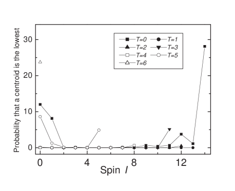
Figure 1: Probability that an energy centroid $\overline{E_{I,T}}$ is the lowest. One sees that this probability is large only when $I$ $and$ $T$ are close to minimum or maximum. Note that the $I_{\rm max}$ value for large $T$ becomes smaller as $T$ increases, and that for 12 nucleons in the $sd$ shell only $I=0$ is possible when $T=6$.

We have obtained $\overline{E_{I,T}}$ based on $\overline{E_{I}}$’s of systems with $N=12$ ($N_{p}=6,7,\cdots 12,N_{p}+N_{n}=12$) and those with $N=8$ ($N_{p}=4,5,\cdots 8,N_{p}+N_{n}=8$) in the $sd$ shell. In Fig. 1 we present out results of ${\cal P}(I,T)$ which is the probability that the lowest energy centroid has spin $I$ and isospin $T$. One easily notices that ${\cal P}(I,T)$ is sizable only when both $I$ and $T$ are close to their minimum or maximum values. To see this more clearly, we list in Table I the values of $\sum_{I}{\cal P}(I,T)$, where we see that $\sum_{I}{\cal P}(I,T)$ is very small when the value of $T$ is not close to its minimum or maximum value. We note here that $\sum_{I}{\cal P}(I,T)$ does not equal ${\cal P}(T)$, the probability that $\overline{E_{T}}$ (the energy centroid of all states with isospin $T$) is the lowest.

The feature that $\sum_{I}{\cal P}(I,T)$ is large only when $T$ and $I$ are close to their minimum or maximum values is very similar to that of ${\cal P}(I)$ discussed in Refs. Zhaox ; Zhao-2005 , and more generally, to that of ${\cal P}(\lambda)$ discussed in Ref. Kota2 where $\lambda$ denotes irreducible representation of states in interacting boson models suggested in Refs. Arima0 ; Iachello .

Table 1: $\sum_{I}{\cal P}(I,T)$ for eight and twelve particles in the $sd$ shell. One sees that $\sum_{I}{\cal P}(I,T)$ is very small when the value of $T$ is not close to $T_{\rm min}$ or $T_{\rm max}$. We define $\overline{E_{T}}=\sum_{I}(2I+1)\overline{E_{I,T}}D_{IT}/\left(\sum_{I}(2I+1)D_{IT}\right)$ and ${\cal P}(T)$ be the probability for $\overline{E_{T}}$ to be the lowest in energy, and note here that ${\cal P}(T)$ does not equal $\sum_{I}{\cal P}(I,T)$.

$T$	0	1	2	3	4	5	6
$N=8$
	47.1	11.0	5.5	2.2	34.2
$N=12$
	57.9	0.8	0.5	4.9	0.5	13.6	21.8

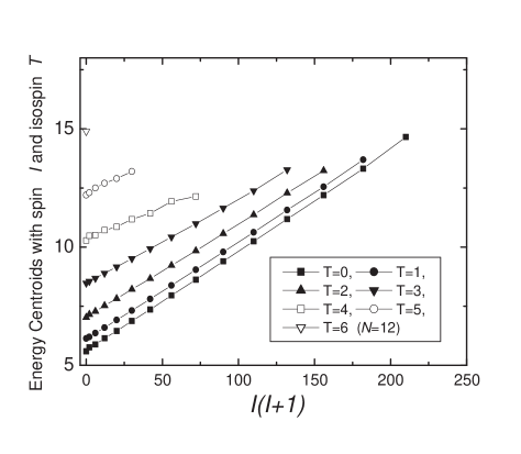
Figure 2: $\langle\overline{E_{IT}}\rangle_{\rm min}$ versus $I(I+1)$ values. Here $\langle\overline{E_{IT}}\rangle_{\rm min}$ are obtained by averaging the $\overline{E_{IT}}$ over the cases in which the lowest $\overline{E_{IT}}$ has $I=0,1$ and $T=0$. One sees that $\langle\overline{E_{IT}}\rangle_{\rm min}$ is proportional to $I(I+1)$ approximately, and that $\langle\overline{E_{IT}}\rangle_{\rm min}$ with different $T$ values are different: those with larger $T$ being systematically higher.

As in earlier works, we investigate here the relation $\langle\overline{E_{I}}\rangle_{\rm min}\propto I(I+1)$, where $\langle\overline{E_{I}}\rangle_{\rm min}$ is obtained by averaging $\overline{E_{I}}$ over the cases of the ensemble in which $\overline{E_{I}}~{}(I\sim I_{\rm min})$ is the lowest in energy. From Fig. 2, one sees that this relation is very robust with inclusion of the isospin degree of freedom $T$, i.e., $\langle\overline{E_{I,T}}\rangle_{\rm min}\propto I(I+1)$. A new and interesting observation here is that the $\langle\overline{E_{I,T}}\rangle_{\rm min}$ results, which are obtained by averaging over the case in which $\overline{E_{IT}}~{}(I\sim I_{\rm min},T\sim T_{\rm min})$ is the lowest energy, can be classified according to their $T$ values: the values of $\langle\overline{E_{I,T}}\rangle_{\rm min}$ with larger $T$ are systematically higher.

As we will show later, closer inspection of our calculated results confirms that $\overline{E_{T}}=\sum_{I}(2I+1)\overline{E_{I,T}}D_{IT}/\left(\sum_{I}(2I+1)D_{IT}\right)=E_{0}+CT(T+1)$ for each individual run, which was shown by French many years ago French1 ; French2 . $D_{T}=\sum_{I}(2I+1)D_{IT}$. Note that the $(2I+1)$ factor is essential for proper definition of fixed-$T$ centroids.

Below we discuss fixed-$T$ centroids by propagation equations. With nucleons occupying say $(j_{1},j_{2},\ldots)$ orbits, the spectrum generating algebra is $U({\cal N})$, ${\cal N}=\sum_{i}\,2(2j_{i}+1)$ with the factor 2 appearing due to isospin. For $n$ nucleons with isospin $T$, the $T$ quantum number labels the irreducible representations (irreps) of $SU(2)$ algebra that appears in the direct product (space-isospin) subalgebra $U({\cal N}/2)\otimes SU(2)$ of $U({\cal N})$. Then the irreps of $U({\cal N}/2)$ are completely specified by $(n,T)$. A one plus two-body hamiltonian $H=h(1)+V(2)$, which preserves angular momentum and isospin is defined by the single particle energies (spe) $\epsilon_{i}$ and by the two-body matrix elements $V^{Jt}_{ijkl}=\langle(kl)Jt\mid V(2)\mid(ij)Jt\rangle$, where $|(ij)Jt\rangle$ are anti-symmetrized two particle states. With $H=h(1)+V(2)$, $\overline{E_{T}}$ are polynomials in the scalars particle number $n$ and $T(T+1)$: $\overline{E_{T}}=a_{0}+a_{1}\,n+a_{2}n^{2}+a_{3}T(T+1)$; see Refs. French1 ; French2 . Solving for the $a_{i}$’s using $\overline{E_{(n,T)}}$ for $n\leq 2$, one obtains the following propagation formula

$$\overline{E_{T}}=n\langle h(1)\rangle^{1,\frac{1}{2}}$$

$$+\left\{\frac{n(n+2)}{8}-\frac{T(T+1)}{2}\right\}\langle V(2)\rangle^{2,0}$$

$$+\left\{\frac{3n(n-2)}{8}+\frac{T(T+1)}{2}\right\}\langle V(2)\rangle^{2,1}~{}$$ (3)

with

$$\langle h(1)\rangle^{1,\frac{1}{2}}=\frac{1}{\cal N}\sum_{i}2(2j_{i}+1)\epsilon_{i}~{},$$

$$\langle V(2)\rangle^{2,t}=\frac{1}{D_{t}}\sum_{i\geq j;J}V^{Jt}_{ijij}(2J+1)~{}.$$

From Eq. (3), $\overline{E_{T_{\rm max}}}-\overline{E_{T}}=\frac{1}{2}\{\langle V(2)\rangle^{2,1}-\langle V(2)\rangle^{2,0}\}\;\{T_{\rm max}(T_{\rm max}+1)-T(T+1)\}$. With the interaction matrix elements $V_{ijij}^{J,t}$ chosen to be zero centered independent Gaussian random variables, ground states will have $T=0$ or $T_{\rm max}$, with $50$% probability for each of them.

III energy centroids of spin $I$ states under random three-body interactions

The outcome of random three-body interactions for $sd$ bosons was first studied by Bijker and Frank in Ref. Bijker , where it was found that the inclusion of random three-body interactions does not drastically change the pattern of spin $I$ distribution in the ground states, in comparison with the results calculated by using random two-body interactions, if boson number $n$ is much larger than three. In this section we study whether or not the pattern of $\overline{E_{I}}$ becomes different if one includes random three-body interactions. To highlight the feature of $\overline{E_{I}}$ with three-body part, we use a Hamiltonian with only three-body interactions defined in Appendix B. The three-body interaction parameters are chosen to be random and follow the Gaussian distribution.

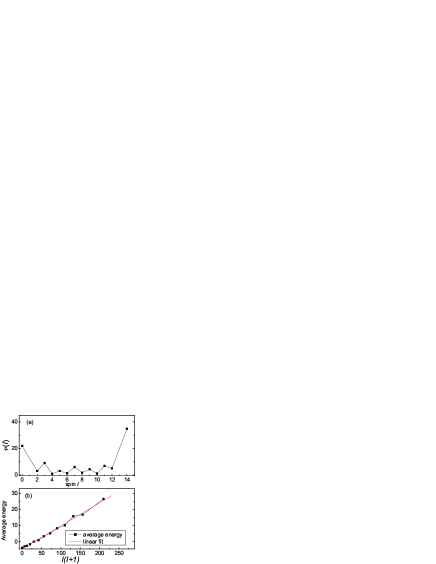
Figure 3: (a) ${\cal P}(I)$ with pure random three-body interactions for $sd$ boson systems. One sees that ${\cal P}(I)$ is large when $I$ equals $I_{\rm max}$ and $I_{\rm min}$. ${\cal P}(I)$ also exhibits an odd-even staggering: ${\cal P}(I)$ is relatively large for odd $I$ values and small for even $I$ values. (b) $\overline{E_{I}}$ versus $I(I+1)$. One sees that $\overline{E_{I}}\simeq E_{0}+CI(I+1)$ for $sd$ bosons with three body random interactions. In this figure the total boson number $n$ is 7. Similar results are obtained for $n=6-20$.

Figure 3(a) is a typical example of probability (denoted by ${\cal P}(I)$) for $\overline{E_{I}}$ to be the lowest with pure random three-body interactions of seven $sd$ boson systems. Interestingly but as expected, one sees that ${\cal P}(I)$ is large when $I\sim 0$ or $I\sim I_{\rm max}$. One also sees a very apparent odd-even staggering of ${\cal P}(I)$ values, i.e., ${\cal P}(I)$ is large when $I$ is odd and relatively smaller when $I$ is even. This behavior was also noticed and discussed in Ref. Zhaox when only the TBRE was used.

Figure 3(b) presents $\langle\overline{E_{I}}\rangle_{\rm min}$ versus $I(I+1)$ for seven $sd$ bosons. A linear correlation between $\langle\overline{E_{I}}\rangle_{\rm min}$ and $I(I+1)$ can be easily seen.

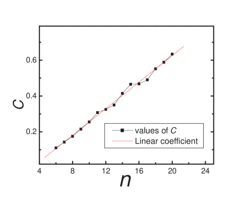
Figure 4: The value of $C$ in the relation $\langle\overline{E_{I}}\rangle_{\rm min}\simeq CI(I+1)$ for $sd$-boson systems versus boson number $n$. We see that the value of $C$ is approximately proportional to particle number $n$.

A difference between $\langle\overline{E_{I}}\rangle_{\rm min}$ under the TBRE and that obtained by using random three-body interactions is found when one studies the correlation $\langle\overline{E_{I}}\rangle_{\rm min}=CI(I+1)$ for $sd$-boson systems with different particle number $n$. For the case by using the TBRE, the value of coefficient $C$ is not sensitive to particle number $n$ but sensitive to the single-particle levels in which the valence particles are active; for systems in which one takes random three-body interactions, the situation becomes different. In Fig. 4 we see that the value of $C$ increases with boson number $n$ linearly with small fluctuations.

Now let us investigate the energy centroids of spin $I$ states by using propagation equations for random three-body interactions. In order to understand the particle number dependence seen in Fig. 4, we consider spin $I$ centroids $\overline{E_{I}}$ generated by random three-body hamiltonians for identical nucleons in a single-$j$ shell. Firstly $\overline{E_{I}}$’s correspond to averages over the space defined by the irreps $n$ and $I$ of $U(2j+1)$ and $SO(3)$ respectively in $U(2j+1)\supset SO(3)$. We start with the approximate formula (see Eq. (7) in Ref. Kota ),

$$\overline{E_{I}}=\left[\langle H(3)\rangle^{n}-\frac{3}{2}\frac{\langle I_{z}^{2}\widetilde{H(3)}\rangle^{n}}{\langle I_{z}^{2}\rangle^{n}}\right]$$

$$+\frac{1}{2}\frac{\langle I_{z}^{2}\widetilde{H(3)}\rangle^{n}}{\left[\langle I_{z}^{2}\rangle^{n}\right]^{2}}I(I+1)$$ (4)

which should be valid for $j>>n>>3$. In Eq. (4), $\langle H(3)\rangle^{n}$ is the average of $H$ over $n$ particle space and $\widetilde{H}$ is $H$ with the average part removed (this is made more clear ahead). Denoting three particle antisymmetric states by $|(j)^{3};\alpha I\rangle$ with $\alpha$ being the extra label required to completely specify the states, diagonal $3$-particle matrix elements of $H(3)$ are $G_{\alpha J}=\langle(j)^{3};\alpha J\mid H(3)\mid(j)^{3};\alpha J\rangle$.

To proceed further it is necessary to consider the tensorial decomposition of $I^{2}$ and $H$ operators with respect to $U(2j+1)$ and the tensors are denoted by $\nu$ French1 ; French2 . A general $k$-body operator will have $\nu=0$, $1$, $\ldots$, $k$ parts. However for a single $j$ shell the $\nu=1$ part will be zero. Thus $I^{2}=(I^{2})^{\nu=0}+(I^{2})^{\nu=2}$ and $H(3)=H^{\nu=0}(3)+H^{\nu=2}(3)+H^{\nu=3}(3)$. The $\langle H\rangle^{n}$ and $\langle I_{z}^{2}\rangle^{n}=\frac{1}{3}\langle I^{2}\rangle^{n}$ are generated by the $\nu=0$ parts, and

$$\langle I_{z}^{2}\rangle^{n}=\frac{1}{3}\langle I^{2}\rangle^{n}$$

$$=\frac{1}{6}\,n(2j+1-n)(j+1)\simeq\frac{n}{3}j(j+1)~{}.$$ (5)

Note that $\widetilde{H}=H-H^{\nu=0}$, and $\langle I^{2}\widetilde{H(3)}\rangle^{n}=\langle(I^{2})^{\nu=2}H^{\nu=2}(3)\rangle^{n}=\langle(I^{2})^{\nu=2}H(3)\rangle^{n}$. It should be recognized French1 that $H^{\nu=2}(3)=(\hat{n}-2)F^{\nu=2}(2)$, where $F$ is a two-body operator with rank $\nu=2$ and $\hat{n}$ is number operator. For our purpose, it is not necessary to know the exact form of the $F$ operator. The propagation equation for the $n$ particle average $\langle(I^{2})^{\nu=2}F^{\nu=2}(2)\rangle^{n}$ is well known (see for example Eq. (A2) of Ref. Kota ). Using this we obtain

$$\langle(I^{2})^{\nu=2}H(3)\rangle^{n}=\frac{n(n-1)(n-2)(2j+1-n)(2j-n)}{2(2j-1)(2j-2)}$$

$$~{}~{}~{}~{}~{}~{}~{}~{}~{}~{}~{}~{}~{}~{}\times\langle(I^{2})^{\nu=2}F^{\nu=2}(2)\rangle^{2}~{}.$$ (6)

Putting $n=3$ on both sides of Eq. (6), the average involving $F$ can be eliminated and this gives

$$\langle(I^{2})^{\nu=2}H(3)\rangle^{n}=\frac{n(n-1)(n-2)}{6(2j-2)(2j-3)}$$

$$~{}~{}~{}~{}~{}~{}~{}~{}~{}(2j+1-n)(2j-n)\langle(I^{2})^{\nu=2}H(3)\rangle^{3}~{}.$$ (7)

As given in Ref. Kota , $(I^{2})^{\nu=2}=I^{2}-\frac{\hat{n}}{2}(2j+1-\hat{n})(j+1)$. Combining Eq. (7) with Eqs. (4) and (5) give the final formula for $\overline{E_{(n,I)}}$ with the $I(I+1)$ term carrying linear $n$ dependence

$$\overline{E_{(n,I)}}\simeq E_{0}$$

$$+\frac{3n}{2}\left[\frac{\sum_{\alpha,J}\{J(J+1)-3j(j+1)\}G_{\alpha J}(2J+1)}{[j(j+1(2j+1)]^{2}(2j+1)}\right]$$

$$~{}~{}~{}~{}~{}~{}~{}~{}~{}~{}~{}~{}~{}~{}~{}\times I(I+1)~{},$$ (8)

where $E_{0}$ is a constant determined by $G_{\alpha J}$, $n$ and $j$. The form of $E_{0}$ is given in Appendix A. The second term in Eq. (8) clearly gives a linear $n$-dependence for $C$. This dependence, as seen from the unitary decomposition, comes from the $\nu=2$ part of $H(3)$ which in turn is responsible for the $I(I+1)$ term.

Similarly, one investigates $\overline{E_{(n,I)}}$ versus $I(I+1)$ for bosons with spin $l$. Eq. (4) remains the same but

$$\langle I_{z}^{2}\rangle^{n}=\frac{1}{6}n(2l+1+n)l$$

$$\langle I_{z}^{2}\widetilde{H(3)}\rangle^{n}=$$

$$\frac{1}{3}\left[\frac{n(n-1)(n-2)(2l+1+n)(2l+2+n)}{(2l+1)(2l+2)(2l+3)(2l+4)(2l+5)}\right]\times$$

$$\sum_{\alpha,L}\{L(L+1)-3l(l+2)\}G_{\alpha L}(2L+1)~{}.$$ (9)

Then one obtains

$$\overline{E_{(n,I)}}\simeq E^{\prime}_{0}+n\frac{6}{l^{2}(2l+1)(2l+2)\cdots(2l+5)}$$

$$~{}~{}\sum_{\alpha,L}\left[L(L+1)-3l(l+2)\right]G_{\alpha L}\times I(I+1)~{},$$ (10)

where $G_{\alpha L}$ are three-body matrix elements for bosons with spin $l$. For $d$ bosons there are five three-body matrices with $L=0,2,3,4$ and 6, respectively. By using Eq.(10), one obtains the value of coefficient $C$ in the relation $\langle\overline{E_{I}}\rangle_{\rm min}\simeq CI(I+1)$ for $d$ boson systems:

$$C=\sqrt{\frac{2}{\pi}}\frac{6n}{l^{2}(2l+1)(2l+2)\cdots(2l+5)}$$

$$\sqrt{\sum_{L}\left((L(L+1)-3l(l+2))(2L+1)\right)^{2}}$$

$$=\frac{\sqrt{997\pi}}{1680}n\simeq 0.03331n~{},$$ (11)

where the constant $\sqrt{\frac{2}{\pi}}$ comes from the integral

$$\frac{2}{\sqrt{2\pi}}\int^{\infty}_{0}x{\rm exp}(-\frac{x^{2}}{2})~{}{\rm d}x~{}.$$

The value of $C$ obtained by our numerical experiments (1000 runs of the ensemble with random three-body interactions for $d$ boson systems of $n=6$-20) is $0.03499n$. The value of $C$ is therefore reasonably reproduced by the propagation equation (which predicts $C=0.03331n$ as discussed above).

IV Energy centroids with fixed irreducible representation

In this section we consider two interesting examples: (i) energy centroids with fixed irreps of the $SU_{sd}(3)\oplus SU_{pf}(3)$ limit of $sdpf$IBM which was mentioned in Ref. Kota2 ; (ii) energy centroids with fixed Wigner’s spin-isospin supermultiplet $SU(4)$ irreps for $(2s1d)$ shell nuclei.

Let us first consider energy centroids with fixed irreps $[n_{sd}(\lambda_{sd}\mu_{sd}):n_{pf}(\lambda_{pf}\mu_{pf})]$ of $[U_{sd}(6)\supset SU_{sd}(3)]\oplus[U_{pf}(10)\supset SU_{pf}(3)]$ subalgebra of the spectrum generating algebra (SGA) $U_{sdpf}(16)$ of $sdpf$IBM; see Refs. Long for details of the $SU(3)$ limit of $sdpf$IBM. Given a one plus two-body $sdpf$ hamiltonian, with boson number $n=n_{sd}+n_{pf}$ where $n_{sd}$ and $n_{pf}$ are number of bosons in $sd$ and $pf$ orbits, the propagation equation for energy centroids can be written as

$$\overline{E_{n_{sd}(\lambda_{sd}\mu_{sd})\,:\,n_{pf}(\lambda_{pf}\mu_{pf})}}$$ (17)

$$= a_{0}+a_{1}n_{sd}+a_{2}n_{pf}+a_{3}\left(\begin{array}[]{c}n_{sd}\\ 2\end{array}\right)+a_{4}\left(\begin{array}[]{c}n_{pf}\\ 2\end{array}\right)$$

$$+a_{5}n_{sd}n_{pf}+a_{6}C_{2}(\lambda_{sd}\mu_{sd})+a_{7}C_{2}(\lambda_{pf}\mu_{pf})\;,$$

where $C_{2}(\{f\})$ in this section denotes the eigenvalue of the quadratic Casimir invariant of a given irrep $\{f\}$. For irreps $(\lambda\mu)$ of SU(3) it is given by $C_{2}(\lambda\mu)=\lambda^{2}+\mu^{2}+\lambda\mu+3(\lambda+\mu)$. The final propagation equation can be obtained by solving for the $a_{i}$’s in terms of the centroids with $n\leq 2$. We give this equation in the Appendix A.

In order to calculate energy centroids using Eq. (41), the reductions $n_{sd}\rightarrow(\lambda_{sd}\mu_{sd})$ and $n_{pf}\rightarrow(\lambda_{pf}\mu_{pf})$ are needed. For $sd$ bosons the reductions are well known Arima0 ; Iachello and for the $pf$ system the reductions are obtained using the method given in Ref. Kota-5 . Following the results for $sd$IBM-$T$ and $sd$IBM-$ST$ energy centroids given in Ref. Kota2 , we consider the basic energy centroids $\langle H\rangle^{n_{sd}(\lambda_{sd}\mu_{sd}):n_{pf}(\lambda_{pf}\mu_{pf})}$ with $n\leq 2$ as independent zero centered (with unit variance) Gaussian random variables, instead of considering the single-particle energies and two-body matrix elements in $sdpf$ space as random variables.

With 1000 samples, the probabilities for the energy centroid with a given $[n_{sd}(\lambda_{sd}\mu_{sd}):n_{pf}(\lambda_{pf}\mu_{pf})]$ irrep to be lowest are calculated for boson numbers $n=8$, $9$ and $10$ and the results are shown in Fig. 5. Firstly it is seen that the irreps with the lowest and highest $n_{sd}$ carry most of the probability, about $84$%. For each of the other $n_{sd}$ the probability is $1-3$%. Moreover for the lowest and highest $n_{sd}$, the probability splits into the lowest and highest $SU(3)$ irreps. For $n_{sd}=0$ obviously $(\lambda_{sd}\mu_{sd})=(00)$ and the probability for highest (according to the eigenvalue of the $SU_{pf}(3)$ quadratic Casimir invariant) $SU_{pf}(3)$ irreps $(3n,0)$ is $\sim 24$% and for the lowest irreps it is $\sim 19$%. The lowest irreps for $n_{pf}=n=8$, $9$ and $10$ are $(\lambda_{pf}\mu_{pf})=(00)$, $(30)+(03)$ and $(00)$, respectively. Similarly, for $n_{sd}=n$, the highest $SU_{sd}(3)$ irreps are $(2n,0)$ with probability $24$% and the lowest irreps are $(02)$, $(00)$ and $(20)$ respectively for $n_{sd}=n=8$, $9$ and $10$ with probability $\sim 17$%. Thus the results in Fig. 5 show that the energy centroids with the lowest and highest $[n_{sd}(\lambda_{sd}\mu_{sd}):n_{pf}(\lambda_{pf}\mu_{pf})]$ irreps carry most of the probability just as with $I$ and $IT$ energy centroids considered in this paper and in many other examples considered in Refs. [7-12].

Now let us come to the second example, energy centroids with fixed $SU(4)-(ST)$ irreps for the $(2s1d)$ shell model. For $(2s1d)$ shell nuclei, spin-ispopin supermultiplet $SU(4)$ algebra appears in the direct product subalgebra $U(6)\otimes SU(4)$ of $U(24)$ SGA.

We first note that $U(6)$ generates the orbital part and $SU(4)$ generates spin-isospin $(ST)$ quantum numbers via $SU_{ST}(4)\supset SU_{S}(2)\otimes SU_{T}(2)$. For a given number of nucleons $n$, the allowed $U(4)$ irreps are $\{f\}=\{f_{1},f_{2},f_{3},f_{4}\}$ with $f_{1}\geq f_{2}\geq f_{3}\geq f_{4}\geq 0$, $f_{1}\leq 6$ and $f_{1}+f_{2}+f_{3}+f_{4}=n$ and the $U(6)$ irreps, by direct product nature, are $\{\tilde{f}\}$, the transpose of $\{f\}$. It is important to note that the equivalent $SU(4)$ irreps are $\{f_{1}-f_{4},f_{2}-f_{4},f_{3}-f_{4}\}$. With these, from now on we will use $U(4)$ and the irreps $\{f\}$. It is well known that a totally symmetric $U(4)$ irrep $\{\lambda\}\rightarrow(ST)=(\frac{\lambda}{2},\frac{\lambda}{2})$, $(\frac{\lambda}{2}-1,\frac{\lambda}{2}-1)$, $\ldots$, $(00)$ or $(\frac{1}{2},\frac{1}{2})$. Using this result and expanding a given $U(4)$ irrep into totally symmetric $U(4)$ irreps will give easily $\{f\}\rightarrow(ST)$ reductions. Just as the fixed-$T$ energy centroids propagate, the fixed $\{f\}(ST)$ energy centroids $\overline{E_{\{f\}(ST)}}$ for a one plus two-body hamiltonian propagate as the available scalars of maximum body rank 2 are $1$, $\hat{n}$, $\hat{n}^{2}$, $C_{2}(U(4))$, $S^{2}$ and $T^{2}$ and the centroids for $n\leq 2$ are also six in number. The propagation equation, with $C_{2}(\{f\})=\sum_{i}\,f_{i}^{2}+3f_{1}+f_{2}-f_{3}-3f_{4}$ for $U(4)$ irrep $\{f\}$, was first discussed in Ref. Haq and we present it in Appendix A, for the sake of convenience.

Figure 5: Probabilities for $sdpf$IBM centroid energies with fixed-$[n_{sd}(\lambda_{sd}\mu_{sd}):n_{pf}(\lambda_{pf}\mu_{pf})]$ irreps to be lowest in energy vs $n_{sd}$ for systems of $n=8$, $9$ and $10$ bosons. For $n_{sd}=0$ ($n_{pf}=n$) and $n_{sd}=n$ ($n_{pf}=0$) the probabilities for $(\lambda_{pf}\mu_{pf})$ [$(\lambda_{sd}\mu_{sd})=(00)$] and $(\lambda_{sd}\mu_{sd})$ [$(\lambda_{pf}\mu_{pf})=(00)$] are shown in the figure. However for $0<n_{sd}<n$, the probabilities shown are the sum of the probabilities for the $[n_{sd}(\lambda_{sd}\mu_{sd}):n_{pf}(\lambda_{pf}\mu_{pf})]$ irreps; for each $n_{sd}$ and $n_{pf}=n-n_{sd}$ there are $3-4$ $SU(3)$ irreps but they are not shown in the figure to avoid clustering of too many points. Filled circles, squares and stars are joined by lines to guide the eyes. See text for further details.

Just as in the $sdpf$ example, we consider the basic energy centroids $\langle H\rangle^{\{f\}(ST)}$ with $n\leq 2$ as independent zero centered (with unit variance) Gaussian random variables, instead of using $\epsilon_{i}$ and $V^{Jt}_{ijkl}$ as random variables, and study the $\{f\}(ST)$ structure of the ground states.

Using 1000 samples, the probability for a given fixed-$\{f\}(ST)$ energy centroid to be lowest in energy is calculated and the results are shown in Fig. 6 for $n=8$, $9$, $10$ and $12$. The probabilities split into three $U(4)$ irreps (other irreps carry $<1$% probability) for $n=8$, $9$ and $10$, and the corresponding $(ST)$ values are as shown in Fig. 6. Energy centroids with the lowest and highest $U(4)$ irreps carry $\sim 25$% and $\sim 40$%, respectively. The lowest irreps are $\{2^{4}\}$, $\{32^{3}\}$ and $\{3^{2}2^{2}\}$ respectively for $n=8$, $9$ and $10$ and the highest irreps are $\{6,n-6\}$. The third irreps $\{4^{2}\}$, $\{54\}$ and $\{5^{2}\}$, with probability $\sim 32$% for $n=8$, $9$ and $10$, are those that carry $S=n/2$ or $T=n/2$. Besides these, for $n=10$ the irrep $[3^{3}1](00)$ carries $3.7$% probability. For the mid-shell example with $n=12$ the probabilities split into the lowest $\{3^{4}\}$ and highest $\{6^{2}\}$ irreps with $\sim 25$% and $\sim 75$%, respectively. The lowest irrep supports only $(ST)=(00)$ and the probability for the highest irrep splits into $\sim 13$% and $\sim 62$% for $(ST)=(00)$ and $(12,0)+(0,12)$. A very important observation from Fig. 6 is that the probability for the energy centroid with lowest $U(4)$ irrep to be lowest is only $\sim 25$% and it should be noted that the corresponding $SU(4)$ irreps are $\{0\}(00)$, $\{1\}(\frac{1}{2}\frac{1}{2})$ and $\{1^{2}\}(10)+(01)$ for $n=4k$, $4k+1$ and $4k+2$, respectively, with $k$ being a positive integer. In fact as discussed in Ref. Zhao-Scholten , realistic interactions give ground state wavefunctions having overlap of $\sim 90$% with these irreps, i.e. very high probability for $\alpha$-cluster structure. However detailed calculations in Ref. Zhao-Scholten showed that random interactions give a very small probability for $\alpha$ clustering. The same result has been brought out in a simple and easy manner by the $\{f\}(ST)$ energy centroids.

Finally we point out that the present study extends easily to $(2p1f)$-shell nuclei by changing the restriction $f_{1}\leq 6$ to $f_{1}\leq 10$ in enumerating the $U(4)$ irreps.

Figure 6: Probabilities for $(2s1d)$ shell centroid energies with fixed $\{f\}(ST)$ irreps to be lowest in energy vs $C_{2}(\{f\})$. Results are shown for nucleon numbers $n=8$, $9$, $10$ and $12$. The irreps carrying probability less than $1$% are not shown in the figure. The $U(4)$ irreps $\{f\}$ for the results in the figure are given in the text. The corresponding $(ST)$ values are shown in the figure as $(2S\,2T)$. Filled circles, filled squares, open circles and open squares are joined by lines to guide the eyes.

V Discussion and summary

In this paper we studied the behavior of energy centroids in the presence of random interactions. First we show that results of energy centroids are robust regardless of inclusion of isospin, based on numerical calculations. We find that $\langle\overline{E_{IT}}\rangle_{\rm min}$ (and $\langle\overline{E_{IT}}\rangle_{\rm max}$) values can be classified according to their $T$ values. The simple relation, $\overline{E_{T}}=E_{0}+CT(T+1)$ for each individual run, is confirmed and discussed. We see $\overline{E_{IT}}$ with both neutrons and protons shows a similar pattern to that of $\overline{E_{I}}$ with only identical particles discussed in earlier works.

Second, we find in this paper that for $sd$ boson systems the feature of $\overline{E_{I}}$’s is robust with inclusion of random three-body interactions. Results of ${\cal P}(I)$, the probability for $\overline{E_{I}}$ to be the lowest in energy, and $\langle\overline{E_{I}}\rangle_{\rm min}$ (and $\langle\overline{E_{I}}\rangle_{\rm max}$), obtained by using the TBRE, are also applicable to those by using random three-body interactions, except that the value of coefficient $C$ in the relation $\langle\overline{E_{I}}\rangle_{\rm min}\simeq CI(I+1)$ increases linearly with boson number $n$.

Third, such regular patterns can be generalized to energy centroids with given irreducible representations of groups for boson systems as well as fermion systems. We consider energy centroids with fixed irreps of the $SU_{sd}(3)\oplus SU_{pf}(3)$ limit of $sdpf$IBM, and energy centroids with fixed Wigner’s spin-isospin supermultiplet $SU(4)$ irreps for $(2s1d)$ shell nuclei. We see that the lowest and highest irreps $\{f\}$ carry most of the cases that $\overline{E_{I}}$ is the lowest in energy, and the energy centroids propagate via quadratic Casimir invariants.

The above results, such as energy centroids with fixed $T$ value, energy centroids of spin $I$ states under random three-body interactions, energy centroids of fixed irreps of the IBM models and shell models, are discussed by using propagation equations.

Our results suggest that behavior of energy centroids discussed in Refs. [7-12] is a very robust feature for quantum many-body systems interacting by random forces.

Acknowledgement: One of the authors (YMZ) would like to thank the National Natural Science Foundation of China under Grant Nos. 10545001 and 10575070 for supporting this work. Another author (N. Yoshida) is thankful to the financial support by “Academic Frontier” Project and Organization for Research and Development of Innovative Science and Technology (ORDIST) of Kansai University.

Appendix A    Useful formulas in deriving propagation equations

First we present the detailed result of $E_{0}$ in Eq. (9) of Sec. III.

$$E_{0}=\left[\frac{n^{3}}{(2j+1)^{3}}\sum_{\alpha,J}G_{\alpha J}(2J+1)\right.$$

$$~{}~{}~{}~{}~{}~{}~{}~{}-\frac{3n^{2}}{2j(j+1)(2j+1)^{3}}$$

$$~{}~{}~{}~{}~{}~{}~{}~{}\left.\times\sum_{\alpha,J}\{J(J+1)-3j(j+1)\}G_{\alpha J}(2J+1)\right]~{}.$$

Second, we present the propagation equation of energy centroids with fixed irreps $[n_{sd}(\lambda_{sd}\mu_{sd}):n_{pf}(\lambda_{pf}\mu_{pf})]$ of $[U_{sd}(6)\supset SU_{sd}(3)]\oplus[U_{pf}(10)\supset SU_{pf}(3)]$ subalgebra of the spectrum generating algebra (SGA) $U_{sdpf}(16)$ of $sdpf$ IBM. This is obtained by solving $a_{i}$’s in Eq.(17) by centroids with $n\leq 2$.

$$\overline{E_{n_{sd}(\lambda_{sd}\mu_{sd})\,:\,n_{pf}(\lambda_{pf}\mu_{pf})}}$$

$$=\left[1-n_{sd}-n_{pf}\right.$$

$$~{}~{}~{}\left.+\left(\begin{array}[]{c}n_{sd}\\ 2\end{array}\right)+\left(\begin{array}[]{c}n_{pf}\\ 2\end{array}\right)+n_{sd}n_{pf}\right]\overline{E_{0(00):0(00)}}$$ (22)

$$+\left[n_{sd}-2\left(\begin{array}[]{c}n_{sd}\\ 2\end{array}\right)-n_{sd}n_{pf}\right]\overline{E_{1(20):0(00)}}$$ (25)

$$+\left[n_{pf}-2\left(\begin{array}[]{c}n_{pf}\\ 2\end{array}\right)-n_{sd}n_{pf}\right]\overline{E_{0(00):1(30)}}$$ (28)

$$+n_{sd}n_{pf}\overline{E_{1(20):1(30)}}$$

$$+\left[-\frac{5}{9}n_{sd}+\frac{5}{9}\left(\begin{array}[]{c}n_{sd}\\ 2\end{array}\right)+\frac{1}{18}C_{2}(\lambda_{sd}\mu_{sd})\right]\overline{E_{2(40):0(00)}}$$ (31)

$$+\left[\frac{5}{9}n_{sd}+\frac{4}{9}\left(\begin{array}[]{c}n_{sd}\\ 2\end{array}\right)-\frac{1}{18}C_{2}(\lambda_{sd}\mu_{sd})\right]\overline{E_{2(02):0(00)}}$$ (34)

$$+\left[-\frac{3}{5}n_{pf}+\frac{2}{5}\left(\begin{array}[]{c}n_{pf}\\ 2\end{array}\right)+\frac{1}{30}C_{2}(\lambda_{pf}\mu_{pf})\right]\overline{E_{0(00):2(60)}}$$ (37)

$$+\left[\frac{3}{5}n_{pf}+\frac{3}{5}\left(\begin{array}[]{c}n_{pf}\\ 2\end{array}\right)-\frac{1}{30}C_{2}(\lambda_{pf}\mu_{pf})\right]\overline{E_{0(00):2(22)}}~{}.$$ (40)

(41)

Last, we give the propagation equation for energy centroids with fixed spin-isospin SU(4) irreps for the $sd$ shell nuclei. This was first discussed in Ref. Haq .

$$\overline{E_{\{f\}(ST)}}$$ (42)

$$= \left(1-\frac{3}{2}n+\frac{1}{2}n^{2}\right)\,\overline{E_{\{0\}(00)}}+\left(2n-n^{2}\right)\overline{E_{\{1\}(\frac{1}{2}\frac{1}{2})}}$$

$$+\left[-\frac{9}{8}n+\frac{1}{4}n^{2}+\frac{1}{8}C_{2}(\{f\})+\frac{1}{4}S(S+1)\right.$$

$$~{}~{}~{}\left.+\frac{1}{4}T(T+1)\right]\overline{E_{\{2\}(11)}}$$

$$+\left[-\frac{1}{8}n+\frac{1}{8}C_{2}(\{f\})-\frac{1}{4}S(S+1)\right.$$

$$~{}~{}~{}\left.-\frac{1}{4}T(T+1)\right]\overline{E_{\{2\}(00)}}$$

$$+\left[\frac{3}{8}n+\frac{1}{8}n^{2}-\frac{1}{8}C_{2}(\{f\})+\frac{1}{4}S(S+1)\right.$$

$$\left.~{}~{}~{}-\frac{1}{4}T(T+1)\right]\overline{E_{\{1^{2}\}(10)}}$$

$$+\left[\frac{3}{8}n+\frac{1}{8}n^{2}-\frac{1}{8}C_{2}(\{f\})-\frac{1}{4}S(S+1)\right.$$

$$\left.~{}~{}~{}+\frac{1}{4}T(T+1)\right]\overline{E_{\{1^{2}\}(01)}}~{}.$$

Appendix B    Definition of three-body interactions of $sd$ bosons

In this Appendix we present the definition of the three-body Hamiltonian of $sd$ boson systems discussed in Sec. III. We note that the same definition was taken in Ref. Bijker by Bijker and Frank. Discussions of three-body interactions in the interacting boson model can be found in Ref.Iachello .

Our three-body Hamiltonian of $sd$ bosons are given by

$$H_{3}=\sum_{L=0,2,3,4,6}\sum_{i\leq j}\xi_{L_{ij}}\frac{P^{\dagger}_{L_{i}}\cdot P_{L_{j}}+P^{\dagger}_{L_{j}}\cdot P_{L_{i}}}{1+\delta_{ij}}~{},$$ (43)

where

$$P_{0_{1}}^{\dagger}=\frac{1}{6}\left(s^{\dagger}s^{\dagger}s^{\dagger}\right)^{(0)}~{},P_{0_{2}}^{\dagger}=\frac{1}{2}\left(s^{\dagger}d^{\dagger}d^{\dagger}\right)^{(0)}~{},$$

$$P_{0_{3}}^{\dagger}=\frac{1}{6}\left(d^{\dagger}d^{\dagger}d^{\dagger}\right)^{(0)}~{},P_{2_{1}}^{\dagger}=\frac{1}{6}\left(s^{\dagger}s^{\dagger}d^{\dagger}\right)^{(2)}~{},$$

$$P_{2_{2}}^{\dagger}=\frac{1}{2}\left(s^{\dagger}d^{\dagger}d^{\dagger}\right)^{(2)}~{},P_{2_{3}}^{\dagger}=\frac{1}{6}\left(d^{\dagger}d^{\dagger}d^{\dagger}\right)^{(2)}~{},$$

$$P_{3_{1}}^{\dagger}=\frac{1}{6}\left(d^{\dagger}d^{\dagger}d^{\dagger}\right)^{(3)}~{},P_{4_{1}}^{\dagger}=\frac{1}{2}\left(s^{\dagger}d^{\dagger}d^{\dagger}\right)^{(4)}~{},$$

$$P_{4_{2}}^{\dagger}=\frac{1}{6}\left(d^{\dagger}d^{\dagger}d^{\dagger}\right)^{(4)}~{},P_{6_{1}}^{\dagger}=\frac{1}{6}\left(d^{\dagger}d^{\dagger}d^{\dagger}\right)^{(6)}~{}.$$ (44)

The coefficients $\xi_{L_{ij}}$ are random and follow the Gaussian distribution with their widths given by

$$\langle\xi_{L_{ij}}\xi_{L^{\prime}_{i^{\prime}j^{\prime}}}\rangle=(1+\delta_{LL^{\prime}}\delta_{ii^{\prime}}\delta_{jj^{\prime}})/2~{}.$$ (45)

References

- (1) C. W. Johnson, G. F. Bertsch, and D. J. Dean, Phys. Rev. Lett. 80, 2749(1998).
- (2) Y. M. Zhao, A. Arima, and N. Yoshinaga, Phys. Rep. 400, 1 (2004).
- (3) V. Zelevinsky and A. Volya, Phys. Rep. 391, 311 (2004).
- (4) T. Papenbrock and H. A. Weidenmueller, Phys. Rev. Lett. 93, 132503 (2004); AIP Conf. Proc. 777, 140 (2005).
- (5) N. Yoshinaga, A. Arima, and Y. M. Zhao, “Lowest bound energies for random interactions and the origin of spin zero ground state dominance”, preprint (to be published).
- (6) T. Otsuka and N. Shimizu, AIP Conf. Proc. 726, 43 (2004).
- (7) A. Arima, N. Yoshinaga, and Y. M. Zhao, Eur. Phys. J. A 13, 105 (2002); N. Yoshinaga, A. Arima, and Y. M. Zhao, J. Phys. A 35, 8575 (2002).
- (8) Y. M. Zhao, A. Arima, and N. Yoshinaga, Phys. Rev. C 66, 064323(2002).
- (9) Y. M. Zhao, A. Arima, and K. Ogawa, Phys. Rev. C 71, 017304 (2005).
- (10) V. K. B. Kota, Phys. Rev. C 71, 041304 (2005).
- (11) D. Mulhall, A. Volya, and V. Zelevinsky, Phys. Rev. Lett. 85, 4016(2000).
- (12) V. K. B. Kota and K. Kar, Phys. Rev. E 65, 026130 (2002).
- (13) V. Velazquez and A. P. Zuker, Phys. Rev. Lett. 88, 072502 (2002).
- (14) A. Arima and F. Iachello, Ann. Phys. 99, 253 (1976); ibid. 111, 209(1978); ibid. 123, 468 (1979).
- (15) F. Iachello and A. Arima, The Interacting Boson Model (Cambridge University Press, England, 1987).
- (16) R. Bijker and A. Frank, Phys. Rev. C 62, 014303 (2000).
- (17) H. Banerjee and J.B. French, Phys. Lett. 23, 245 (1966); J.B. French, in Isospin in Nuclear Physics, edited by D.H.Wilkinson (North Holland, Amsterdam, 1969), p.259; F.S. Chang, J.B. French, and T.H. Thio, Ann. Phys. (N.Y.) 66, 137 (1971).
- (18) J.C. Parikh, Group Symmetries in Nuclear Structure (Plenum, New York, 1978); S.S.M. Wong, Nuclear Statistical Spectroscopy (Oxford University Press, New York, 1986).
- (19) J. Engel and F. Iachello, Phys. Rev. Lett. 54, 1126 (1985); H.Y. Ji, G.L. Long, E.G. Zhao and S.W. Xu, Nucl. Phys. A 658, 197 (1999).
- (20) V.K.B. Kota, J. of Phys. A 10, L39 (1977); V.K.B. Kota, Physical Research Laboratory Technical Report PRL-TN-97-78 (1978); Mathematics of Computation 39, 302 (1982).
- (21) R. U. Haq and J. C. Parikh, Nucl. Phys. A220, 349 (1974).
- (22) Y.M. Zhao, A. Arima, N. Shimizu, K. Ogawa, N. Yoshinaga, and O. Scholten, Phys. Rev. C 70, 054322 (2004).