Proton polarizations in polarized ³He studied with the $\vec{{}^{3}{\rm He}}({\vec{e}},e^{\prime}p)d$ and $\vec{{}^{3}{\rm He}}({\vec{e}},e^{\prime}p)pn$ processes

Abstract

We study within the Faddeev framework the $\vec{{}^{3}{\rm He}}({\vec{e}},e^{\prime}p)d$ as well as the $\vec{{}^{3}{\rm He}}({\vec{e}},e^{\prime}p)pn$ and $\vec{{}^{3}{\rm He}}({\vec{e}},e^{\prime}n)pp$ reactions in order to extract information on the proton and neutron polarization in polarized ³He. We achieve clear analytical insight for simplified dynamical assumptions and define conditions for experimental access to important ³He properties. In addition we point to the possibility to measure the electromagnetic proton form factors in the process ${}^{3}{\rm He}(e,e^{\prime}p)d$ which would test the dynamical picture and put limits on medium corrections of the form factors.

I Introduction

With the possibility of solving precisely few-nucleon equations and the availability of high precision nucleon-nucleon potentials it is tempting to ask very detailed questions about the properties of light nuclei. Spin dependent momentum distributions of nuclear clusters inside light nuclei have been studied at many places, see for instance Fentometer . Especially the ³He nucleus is interesting. The availability of highly polarized ³He allows one to perform very detailed electron scattering experiments, which, due to the recent progress in the calculations of three-nucleon (3N) bound and scattering states, can be analyzed very precisely. This makes it tempting to extract information on its properties.

In a recent paper spindep we addressed the question whether momentum distributions of polarized proton-deuteron (pd) clusters in polarized ³He could be accessed through the $\vec{{}^{3}{\rm He}}(e,e^{\prime}{\vec{p}})d$ or $\vec{{}^{3}{\rm He}}(e,e^{\prime}{\vec{d}})p$ processes. Final state interactions (FSI) and meson exchange currents (MEC) turned out to destroy the clear picture offered by the plane wave impulse approximation (PWIA) and the assumption of the single nucleon current operator. This we found for most of the cases studied in the kinematical regime below the pion production threshold. Only for small relative pd momenta direct access to the sought ³He properties appeared possible. The $\vec{{}^{3}{\rm He}}(e,e^{\prime}{\vec{p}})d$ or $\vec{{}^{3}{\rm He}}(e,e^{\prime}{\vec{d}})p$ experiments would require, however, measuring the polarizations of the outgoing particles, which is very demanding.

In this paper we would like to investigate theoretically two processes, $\vec{{}^{3}{\rm He}}({\vec{e}},e^{\prime}p)d$ and $\vec{{}^{3}{\rm He}}({\vec{e}},e^{\prime}p)pn$, measured recently at MAMI Achenbach05 and show that under the same PWIA assumption they provide equivalent information about ³He properties. We remind the reader of our formalism in Sec. II. Section III shows our results for the exclusive proton-deuteron breakup of ³He and Sec. IV deals with different aspects of the semi-exclusive $\vec{{}^{3}{\rm He}}({\vec{e}},e^{\prime}p)pn$ reaction. We end with a brief summary in Sec. V.

II Theory

The spin dependent momentum distributions of proton-deuteron clusters inside the ³He nucleus are defined as:

$${\cal Y}(m_{3},m_{d},m_{p};{\vec{q}}\,)\ \equiv\ \left\langle\Psi m_{3}\left||\phi_{d}m_{d}\rangle|{\vec{q}}\,\frac{1}{2}m_{p}\rangle\langle{\vec{q}}\,\frac{1}{2}m_{p}|\langle\phi_{d}m_{d}|\right|\Psi m_{3}\right\rangle,$$ (1)

where ${\vec{q}}$ is the proton momentum (the deuteron momentum is $-{\vec{q}}$); $m_{p}$, $m_{d}$ and $m_{3}$ are spin magnetic quantum numbers for the proton, deuteron and ³He, respectively. These quantities can be written as

$${\cal Y}(m_{3},m_{d},m_{p};{\vec{q}}\,)\,=\,\left|\sum_{\lambda=0,2}\,Y_{\lambda,m_{3}-m_{d}-m_{p}}({\hat{q}})\,C(1I_{\lambda}\frac{1}{2};m_{d},m_{3}-m_{d},m_{3})\right.$$ (2)

$$\left.C(\lambda\frac{1}{2}I_{\lambda};m_{3}-m_{d}-m_{p},m_{p},m_{3}-m_{d})\ H_{\lambda}(q)\right|^{2},$$ (3)

where $H_{\lambda}(q)$ is the overlap of the deuteron state and the ³He state calculated in momentum space Gloecklebook

$$H_{\lambda}(q)\,\equiv\,\sum_{l=0,2}\,\int_{0}^{\infty}dp\,p^{2}\,\phi_{l}(p)\,\langle pq\alpha_{l\lambda}|\Psi\rangle\ \ ,\ \lambda=0,2.$$ (4)

Here $\langle pq\alpha|\Psi\rangle$ are the partial wave projected wave function components of ³He and $\phi_{l}(p)$ are the s- and d-wave components of the deuteron. The set $\alpha_{l\lambda}$ contributes only for the deuteron quantum numbers $s=1$, $j=1$ and $t=0$. Further $I_{\lambda}=\frac{1}{2}$ for $\lambda=0$ and $\frac{3}{2}$ for $\lambda=2$. It is clear that using this quantity $H_{\lambda}(q)$ the spin dependent momentum distribution ${\cal Y}(m_{3},m_{d},m_{p};{\vec{q}}\,)$ can be constructed for any combination of magnetic quantum numbers and any direction ${\hat{q}}$.

In spindep we also showed that under the PWIA treatment and in the non-relativistic limit there are simple relations between different ${\cal Y}$’s and the response functions $W_{i}$, which enter the laboratory cross section for the process ${\vec{e}}+\vec{{}^{3}{\rm He}}\rightarrow e^{\prime}+p+d$. This cross section has the form Donnelly

$$\sigma({\vec{S}},h)\ = \ \sigma_{\rm Mott}\,\left\{\,\left(v_{L}W_{L}+v_{T}W_{T}+v_{TT}W_{TT}+v_{TL}W_{TL}\right)\,\right.$$ (5)

$$+ \left.h\,\left(v_{T^{\prime}}W_{T^{\prime}}+v_{TL^{\prime}}W_{TL^{\prime}}\right)\,\right\}\,\rho,$$

where $\sigma_{\rm Mott}$, $v_{i}$ and $\rho$ are analytically given kinematical factors, $h$ is the helicity of the incoming electron and ${\vec{S}}$ represents the initial ³He spin direction.

This means that both the cross section and the helicity asymmetry $A({\vec{S}})$

$$A({\vec{S}})\equiv\frac{\sigma({\vec{S}},h=+1)-\sigma({\vec{S}},h=-1)}{\sigma({\vec{S}},h=+1)+\sigma({\vec{S}},h=-1)}$$ (6)

for the $\vec{{}^{3}{\rm He}}({\vec{e}},e^{\prime}p)d$ process can be obtained, assuming PWIA, in terms of $H_{\lambda}$, the electromagnetic proton form factors $G_{E}^{p}$ and $G_{M}^{p}$, and simple kinematical quantities. The response functions read

$$W_{L}=\frac{{\,{G_{E}^{p}}}^{2}\,\left({\,{H_{0}(q)}}^{2}+{\,{H_{2}(q)}}^{2}\right)}{4\,\pi}$$ (7)

$$W_{T}=\frac{\left({\,{H_{0}(q)}}^{2}+{\,{H_{2}(q)}}^{2}\right)\,\left({\,{G_{M}^{p}}}^{2}\,{\,{Q}}^{2}+{\,{G_{E}^{p}}}^{2}\,{\,{q_{f}}}^{2}-{\,{G_{E}^{p}}}^{2}\,{\,{q_{f}}}^{2}\,\cos(2\,\,{\theta_{1}})\right)}{8\,{\,{M}}^{2}\,\pi}$$ (8)

$$W_{TT}=\frac{-{\,{G_{E}^{p}}}^{2}\,\left({\,{H_{0}(q)}}^{2}+{\,{H_{2}(q)}}^{2}\right)\,{\,{q_{f}}}^{2}\,\cos(2\,\phi)\,{\sin^{2}(\,{\theta_{1}})}\ }{4\,{\,{M}}^{2}\,\pi}$$ (9)

$$W_{TL}=\frac{{\,{G_{E}^{p}}}^{2}\,\left({\,{H_{0}(q)}}^{2}+{\,{H_{2}(q)}}^{2}\right)\,\,{q_{f}}\,\cos(\phi)\,\sin(\,{\theta_{1}})}{{\sqrt{2}}\,\,{M}\,\pi}$$ (10)

$$W_{T^{\prime}}=\frac{B_{1}\,\cos\theta^{\star}\ +\ B_{2}\,\sin\theta^{\star}\cos(\phi-\phi^{\star})}{48\,\pi\,M^{2}}$$ (11)

$$W_{{TL}^{\prime}}=\frac{{C}_{1}\,\cos(2\phi-\phi^{\star})\,\sin(\theta^{\star})\,+\,{C}_{2}\,\cos(\phi^{\star})\,\sin(\theta^{\star})}{48\,\pi\,M}$$

$$+\ \frac{{C}_{3}\,\cos(\theta^{\star})\,+\,{C}_{4}\,\cos(\phi-\phi^{\star})\,\sin(\theta^{\star})}{48\,\pi\,M}.$$ (12)

The auxiliary quantities $B_{1}$, $B_{2}$, $C_{1}$–$C_{4}$, which appear in the helicity-dependent response functions $W_{{T}^{\prime}}$ and $W_{{TL}^{\prime}}$ in Eqs. (11) and (12) are

$$B_{1}=\,\left({G_{M}^{p}}\,Q\right)^{2}\,\left(2\,{\,{H_{0}(q)}}^{2}+2\,{\sqrt{2}}\,\,{H_{0}(q)}\,\,{H_{2}(q)}+{\,{H_{2}(q)}}^{2}\ \right)\,$$

$$+\ 3\,\left(2\,{\sqrt{2}}\,\,{H_{0}(q)}-\,{H_{2}(q)}\right)\,\,{H_{2}(q)}\,\left({G_{M}^{p}}\,{Q}\right)^{2}\,\cos(2\,\theta)$$

$$-\ 6\,\left(2\,{\sqrt{2}}\,\,{H_{0}(q)}-\,{H_{2}(q)}\right)\,\,{H_{2}(q)}\,{G_{E}^{p}}\,\,{q}\,{G_{M}^{p}}\,{Q}\,\sin(2\,\theta)\,\sin(\,{\theta_{1}})$$ (13)

$$B_{2}=\ -3\,\,\left({G_{M}^{p}}\,Q\right)^{2}\,{H_{2}(q)}\,\left(-2\,{\sqrt{2}}\,\,{H_{0}(q)}+\,{H_{2}(q)}\right)\,\,\sin(2\,\theta)$$

$$-\ 2\,\,{G_{E}^{p}}\,\,{q_{f}}\,{G_{M}^{p}}\,Q\,\left(2\,{\,{H_{0}(q_{f})}}^{2}+2\,{\sqrt{2}}\,\,{H_{0}(q_{f})}\,\,{H_{2}(q_{f})}+{\,{H_{2}(q_{f})}}^{2}\right)\,\sin(\,{\theta_{1}})$$

$$-\ 6\,\,{G_{E}^{p}}\,\,{q_{f}}\,{G_{M}^{p}}\,Q\,\,{H_{2}(q)}\,\left(-2\,{\sqrt{2}}\,\,{H_{0}(q)}+\,{H_{2}(q)}\right)\,\cos(2\,\theta)\sin(\,{\theta_{1}})$$ (14)

$${C}_{1}=3\,\,{G_{E}^{p}}\,\,{G_{M}^{p}}\,\,{H_{2}(q)}\,\left(-4\,\,{H_{0}(q)}+{\sqrt{2}}\,\,{H_{2}(q)}\right)\,\,{Q}$$ (15)

$${C}_{2}=\,{G_{E}^{p}}\,\,{G_{M}^{p}}\,\left(4\,\,{H_{0}(q)}\,\,{H_{2}(q)}-{\sqrt{2}}\,\left(4\,{\,{H_{0}(q)}}^{2}+5\,{\,{H_{2}(q)}}^{2}\ \right)\right)\,\,{Q}$$ (16)

$${C}_{3}=6\,\,{G_{E}^{p}}\,\,{G_{M}^{p}}\,\,{H_{2}(q)}\,\left(-4\,\,{H_{0}(q)}+{\sqrt{2}}\,\,{H_{2}(q)}\right)\,\,{Q}\,\cos(\phi)\,\sin(2\,\theta)$$ (17)

$${C}_{4}=-6\,\,{G_{E}^{p}}\,\,{G_{M}^{p}}\,\,{H_{2}(q)}\,\left(-4\,\,{H_{0}(q)}+{\sqrt{2}}\,\,{H_{2}(q)}\right)\,\,{Q}\,\cos(\phi)\,\cos(2\,\theta).$$ (18)

We assume the reference frame, for which the three-momentum transfer $\vec{Q}\equiv{\vec{k}}-{\vec{k}}^{\,\prime}$ is parallel to $\hat{z}$ and $\hat{y}\equiv\frac{{\vec{k}}^{\,\prime}\times{\vec{k}}}{\mid{\vec{k}}^{\,\prime}\times{\vec{k}}\mid}$, as well as $\hat{x}=\hat{y}\times\hat{z}$. Here ${\vec{k}}$ and ${\vec{k}}^{\,\prime}$ are the initial and final electron momenta. In this system $\theta_{1}$ and $\phi_{1}$ are the polar and azimuthal angles corresponding to the direction of the final proton-deuteron relative momentum $\vec{q}_{f}\equiv\vec{p}_{p}-\frac{1}{3}\vec{Q}$, $\theta$ and $\phi$ are the polar and azimuthal angles corresponding to the direction of $\vec{q}\equiv\vec{q}_{f}-\frac{2}{3}\vec{Q}=\vec{p}_{p}-\vec{Q}=-\vec{p}_{d}$. The initial ³He spin orientation is defined in terms of the $\theta^{\star}$ and $\phi^{\star}$ angles. Further, $Q\equiv\mid\vec{Q}\mid$, $q_{f}\equiv\mid{\vec{q}}_{f}\mid$ and $q\equiv\mid\vec{q}_{f}-\frac{2}{3}\vec{Q}\mid=\mid\vec{p}_{d}\mid$, where $\vec{p}_{p}$ and $\vec{p}_{d}$ are the final proton and deuteron momenta. Finally $M$ is the nucleon mass.

These expressions simplify significantly if the so-called parallel kinematics is assumed, for which the final proton is ejected parallel to $\vec{Q}$. Then $\theta=\theta_{1}=\phi=\phi_{1}=0$ and the response functions given in Eqs. (8)–(12) and (13)–(18) reduce to

$$W_{T}=\frac{\left(\,G_{M}^{p}\,Q\right)^{2}\,\left({\,{H_{0}(q)}}^{2}+{\,{H_{2}(q)}}^{2}\right)\,}{8\,{\,{M}}^{2}\,\pi}$$ (19)

$$W_{TT}=0$$ (20)

$$W_{TL}=0$$ (21)

$$W_{T^{\prime}}=\frac{\left({G_{M}^{p}}\,Q\right)^{2}\,\left(2\,{\,{H_{0}(q)}}^{2}+2\,{\sqrt{2}}\,\,{H_{0}(q)}\,\,{H_{2}(q)}+{\,{H_{2}(q)}}^{2}\ \right)\,\,\cos(\theta^{\star})}{48\,\pi\,M^{2}}$$

$$+\ \frac{3\,\left({G_{M}^{p}}\,{Q}\right)^{2}\,\left(2\,{\sqrt{2}}\,\,{H_{0}(q)}-\,{H_{2}(q)}\right)\,\,{H_{2}(q)}\,\,\cos(\theta^{\star})}{48\,\pi\,M^{2}}$$ (22)

$$W_{{TL}^{\prime}}=\frac{3\,\,{G_{E}^{p}}\,\,{G_{M}^{p}}\,Q\,{H_{2}(q)}\,\left(-4\,\,{H_{0}(q)}+{\sqrt{2}}\,\,{H_{2}(q)}\right)\,\cos(\phi^{\star})\,\sin(\theta^{\star})}{48\,\pi\,M}$$

$$+\ \frac{\,{G_{E}^{p}}\,\,{G_{M}^{p}}\,Q\,\left(4\,\,{H_{0}(q)}\,\,{H_{2}(q)}-{\sqrt{2}}\,\left(4\,{\,{H_{0}(q)}}^{2}+5\,{\,{H_{2}(q)}}^{2}\ \right)\right)\,\cos(\phi^{\star})\,\sin(\theta^{\star})}{48\,\pi\,M}$$

$$-\ \frac{6\,\,{G_{E}^{p}}\,\,{G_{M}^{p}}\,Q\,{H_{2}(q)}\,\left(-4\,\,{H_{0}(q)}+{\sqrt{2}}\,\,{H_{2}(q)}\right)\,\,\cos(\phi^{\star})\,\sin(\theta^{\star})}{48\,\pi\,M}.$$ (23)

This allows us to express the parallel and perpendicular helicity asymmetries in terms of $H_{\lambda}(q)$. For the parallel kinematics they are

$$A_{\parallel}\equiv A(\theta^{\star}=0,\phi^{\star}=0)=$$

$$\frac{\left({G_{M}^{p}}\,Q\,\right)^{2}\,\left({H_{0}(q)}^{2}+4\,{\sqrt{2}}\,{H_{0}(q)}\,{H_{2}(q)}-{H_{2}(q)}^{2}\,\right)\,v_{T^{\prime}}}{3\,\left({H_{0}(q)}^{2}+{H_{2}(q)}^{2}\right)\,\left(2\left({G_{E}^{p}}\,\right)^{2}\,M^{2}\,v_{L}+\left({G_{M}^{p}}\,Q\,\right)^{2}\,v_{T}\right)}$$ (24)

$$A_{\perp}\equiv A(\theta^{\star}=\frac{\pi}{2},\phi^{\star}=0)=$$

$$\frac{-2\,{G_{E}^{p}}\,{G_{M}^{p}}\,M\,Q\,\left({\sqrt{2}}\,{H_{0}(q)}^{2}-4\,{H_{0}(q)}\,{H_{2}(q)}+2\,{\sqrt{2}}\,{H_{2}(q)}^{2}\,\right)\,v_{{TL}^{\prime}}}{3\,\left({H_{0}(q)}^{2}+{H_{2}(q)}^{2}\right)\,\left(2\left({G_{E}^{p}}\,\right)^{2}\,M^{2}\,v_{L}+\left({G_{M}^{p}}\,Q\,\right)^{2}\,v_{T}\right)}$$ (25)

Here, the ³He wave function enters through the combinations

$$P_{1}\equiv\frac{{H_{0}(q)}^{2}+4\,{\sqrt{2}}\,{H_{0}(q)}\,{H_{2}(q)}-{H_{2}(q)}^{2}}{3\,\left({H_{0}(q)}^{2}+{H_{2}(q)}^{2}\right)}$$ (26)

and

$$P_{2}\equiv\frac{{H_{0}(q)}^{2}-2\,{\sqrt{2}}\,{H_{0}(q)}\,{H_{2}(q)}+2\,{H_{2}(q)}^{2}}{3\,\left({H_{0}(q)}^{2}+{H_{2}(q)}^{2}\right)}.$$ (27)

in terms of which

$$A_{\parallel}=\frac{\left({G_{M}^{p}}\,Q\,\right)^{2}\,v_{T^{\prime}}}{2\left({G_{E}^{p}}\,\right)^{2}\,M^{2}\,v_{L}+\left({G_{M}^{p}}\,Q\,\right)^{2}\,v_{T}}\ P_{1}$$ (28)

and

$$A_{\perp}=\frac{-2\,\sqrt{2}\,{G_{E}^{p}}\,{G_{M}^{p}}\,M\,Q\,v_{{TL}^{\prime}}}{2\left({G_{E}^{p}}\,\right)^{2}\,M^{2}\,v_{L}+\left({G_{M}^{p}}\,Q\,\right)^{2}\,v_{T}}\ P_{2}.$$ (29)

The crucial observation is now that $P_{1}$ and $P_{2}$ are related to the spin-dependent momentum distributions ${\cal Y}(m_{3},m_{d},m_{p};{\vec{q}}\,)$ in the following manner

$$P_{1}=\frac{{\cal Y}_{1}-{\cal Y}_{2}}{{\cal Y}_{1}+{\cal Y}_{2}},$$ (30)

where

$${\cal Y}_{1}\equiv{\cal Y}(m_{3}=\frac{1}{2},m_{d}=1,m_{p}=-\frac{1}{2};{\vec{q}}\parallel{\hat{w}})$$

$$=\frac{1}{12\,\pi}\,\left(2H_{0}^{2}+2\sqrt{2}H_{0}H_{2}+H_{2}^{2}\right)=\frac{1}{12\,\pi}\,\left(\sqrt{2}H_{0}+H_{2}\right)^{2}$$ (31)

and

$${\cal Y}_{2}\equiv{\cal Y}(m_{3}=\frac{1}{2},m_{d}=0,m_{p}=\frac{1}{2};{\vec{q}}\parallel{\hat{w}})$$

$$=\frac{1}{12\,\pi}\,\left(H_{0}^{2}-2\sqrt{2}H_{0}H_{2}+2H_{2}^{2}\right)=\frac{1}{12\,\pi}\,\left(H_{0}-\sqrt{2}H_{2}\right)^{2},$$ (32)

where ${\hat{w}}$ denotes the spin quantization axis. Similarly $P_{2}$ can be written as

$$P_{2}=\frac{{\cal Y}_{3}+{\cal Y}_{4}-{\cal Y}_{5}}{{\cal Y}_{3}+{\cal Y}_{4}+{\cal Y}_{5}},$$ (33)

where

$${\cal Y}_{3}\equiv{\cal Y}(m_{3}=\frac{1}{2},m_{d}=-1,m_{p}=-\frac{1}{2};{\vec{q}}\perp{\hat{w}})\ =\ \frac{3}{16\,\pi}\,H_{2}^{2},$$ (34)

$${\cal Y}_{4}\equiv{\cal Y}(m_{3}=\frac{1}{2},m_{d}=1,m_{p}=-\frac{1}{2};{\vec{q}}\perp{\hat{w}})$$

$$=\frac{1}{48\,\pi}\,\left(8H_{0}^{2}-4\sqrt{2}H_{0}H_{2}+H_{2}^{2}\right),$$ (35)

and

$${\cal Y}_{5}\equiv{\cal Y}(m_{3}=\frac{1}{2},m_{d}=0,m_{p}=\frac{1}{2};{\vec{q}}\perp{\hat{w}})$$

$$=\frac{1}{24\,\pi}\,\left(2H_{0}^{2}+2\sqrt{2}H_{0}H_{2}+H_{2}^{2}\right).$$ (36)

The values of spin projections appearing in Eqs. (30) and (33) suggest that $P_{1}$ and $P_{2}$ are just the (negative) proton polarizations for two different proton momenta ${\vec{q}}$ inside polarized ³He. To see that this is true we formally define the proton polarization $P(\vec{q}\,)$

$$P(\vec{q}\,)\equiv\frac{\sum\limits_{m_{p},m_{d}}\left|\left\langle\Psi m_{3}=\frac{1}{2}\right||\phi_{d}m_{d}\rangle|\,{\vec{q}}\,\frac{1}{2}\,m_{p}\,\rangle\right|^{2}\,m_{p}}{\frac{1}{2}\,\sum\limits_{m_{p},m_{d}}\left|\left\langle\Psi m_{3}=\frac{1}{2}\right||\phi_{d}m_{d}\rangle|\,{\vec{q}}\,\frac{1}{2}\,m_{p}\,\rangle\right|^{2}\,}.$$ (37)

Then it is easy to verify that

$$P(\vec{q}\,\parallel{\hat{z}}\,)=-P_{1}$$ (38)

and

$$P(\vec{q}\,\perp{\hat{z}}\,)=-P_{2}.$$ (39)

We also define the total (integrated) proton polarization as

$$P_{\rm int} \equiv \frac{\int d{\vec{q}}\,\sum\limits_{m_{p},m_{d}}\left|\left\langle\Psi m_{3}=\frac{1}{2}\right||\phi_{d}m_{d}\rangle|\,{\vec{q}}\,\frac{1}{2}\,m_{p}\,\rangle\right|^{2}\,m_{p}}{\frac{1}{2}\,\int d{\vec{q}}\,\sum\limits_{m_{p},m_{d}}\left|\left\langle\Psi m_{3}=\frac{1}{2}\right||\phi_{d}m_{d}\rangle|\,{\vec{q}}\,\frac{1}{2}\,m_{p}\,\rangle\right|^{2}\,}$$ (40)

$$= \frac{-\frac{\pi}{24}\,\int\limits_{0}^{\infty}dq\,q^{2}\,\left(\sqrt{2}H_{0}+H_{2}\,\right)^{2}}{\frac{\pi}{4}\,\int\limits_{0}^{\infty}dq\,q^{2}\,\left(H_{0}^{2}+H_{2}^{2}\,\right)}\equiv\frac{-\int\limits_{0}^{\infty}dq\,f_{1}(q)}{\int\limits_{0}^{\infty}dq\,f_{2}(q)}.$$

It is clear that $P_{\rm int}$ is negative. Its numerical value obtained with the nuclear forces used in this paper will be given below.

Thus we can conclude that $P_{1}$ and $P_{2}$, which can be extracted from the parallel and perpendicular helicity asymmetries for the $\vec{{}^{3}{\rm He}}({\vec{e}},e^{\prime}p)d$ process, if the PWIA approximation is valid, are directly the proton polarizations inside the polarized ³He nucleus. In the following we will check this simple dynamical assumption and compare the results based on the PWIA approximation to the results of our full Faddeev calculations. We refer the reader to  report for a detailed description of our numerical techniques, which we do not want to repeat here.

Note that $P_{1}$ and $P_{2}$ are not independent: they are simply related since according to Eqs. (26) and (27)

$$2P_{2}=1-P_{1}.$$ (41)

If Eqs. (28) and (29) are used to obtain the $P_{1}$ and $P_{2}$ values from an experiment, then Eq. (41) gives some measure of the validity of the PWIA assumption, since the relation (41) will in general not hold for the extracted $P_{1}$ and $P_{2}$.

When the argument of $H_{0}$ and $H_{2}$ is small ($q\lesssim 50$ MeV/c), then $H_{2}$ is much smaller than $H_{0}$. Thus one can expect, quite independent of the details of the electron kinematics, that

$$P_{1}\approx P_{2}\approx\frac{1}{3}.$$ (42)

III Results for the $\vec{{}^{3}{\rm He}}({\vec{e}},e^{\prime}p)d$ process

We studied the spin dependent momentum distributions in spindep and had to conclude that (at least in the nonrelativistic regime) one can access these quantities only for rather small pd relative momenta. The results of spindep applied to the $\vec{{}^{3}{\rm He}}(e,e^{\prime}{\vec{p}})d$ and $\vec{{}^{3}{\rm He}}(e,e^{\prime}{\vec{d}})p$ processes but are also valid for the $\vec{{}^{3}{\rm He}}({\vec{e}},e^{\prime}p)d$ reaction, since the same current matrix elements enter in both calculations. The important difference is, however, that a measurement of the latter reaction, which requires only a polarized electron beam and a polarized ³He target, can be easier realized. In fact, this paper is motivated by a very recent experiment  Achenbach05 , where for the first time the electron-target asymmetries $A_{\parallel}$ and $A_{\perp}$ were measured for both the two- and three-body breakup of ³He. Here we restrict ourselves to one electron kinematics from Achenbach05 and show its parameters in Table 1.

Table 1: Electron kinematics from Achenbach05 . E: beam energy, $\theta_{e}$: electron scattering angle, $\omega$: energy transfer, $Q$: magnitude of the three-momentum transfer $\vec{Q}$, $\theta_{Q}$: angle of the three-momentum transfer with respect to the electron beam, $q^{2}$: four-momentum transfer squared, $p_{d}$: magnitude of the deuteron momentum for proton ejected parallel to $\vec{Q}$

E	$\theta_{e}$	$\omega$	$Q$	$\theta_{Q}$	$q^{2}$	$p_{d}$
MeV	deg	MeV	MeV/c	deg	(GeV/c)2	MeV/c
735	50	179	569	48.5	0.29	5

The dynamical input for our calculations is the nucleon-nucleon force AV18 AV18 alone or together with the 3N force UrbanaIX UrbanaIX . We include in addition to the single nucleon current the $\pi$- and $\rho$-like two-body currents linked to the AV18 force, following Riska85

Two-body electron induced breakup of ³He is a very rich process. For example, the description of the deuteron-knockout is not possible within the simplest PWIA approximation and complicated rescattering effects as well as the details of the nuclear current operator play there an important role. A much simpler dynamical picture is expected in the vicinity of the proton knock-out peak. We focus on this angular region and show in Fig. 1 the proton angular distribution for the selected electron configuration.

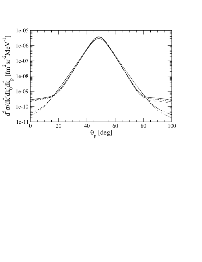
Figure 1: Proton angular distribution for the configuration from Table 1. The proton scattering angle $\theta_{p}$ is defined with respect to the electron beam so the maximum corresponds to the virtual photon direction $\vec{Q}$. The double-dot-dashed curve represents the prediction based on PWIA. The dot-dashed curve is obtained under the assumption of PWIAS (which practically overlaps with PWIA), the dotted curve takes the full FSI into account but neglects MEC and 3NF effects. The $\pi$- and $\rho$-like two-body densities are accounted for additionally in the dashed curve (which overlaps with FSI), and finally, the full dynamics including MEC and the 3N force is given by the solid curve.

The FSI effects for strictly parallel kinematics amount to 5-7 %. Note that the PWIA results shown in Fig. 1 are obtained without inclusion of a 3N force but the full results including the 3N force required both the initial and the final state to be calculated with this dynamical component. The 3N force effects come mainly from the initial bound state and altogether reach almost 20 % at $\theta_{p}=\theta_{Q}$. Note that in this case MEC do not play a big role.

Let us now turn to the helicity asymmetries shown in Figs. 2 and 3.

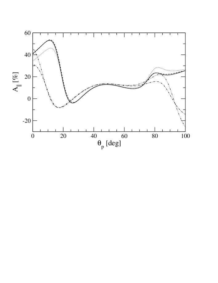
Figure 2: The parallel helicity asymmetry $A_{\parallel}$ for the configuration from Table 1. Curves as in Fig. 1.

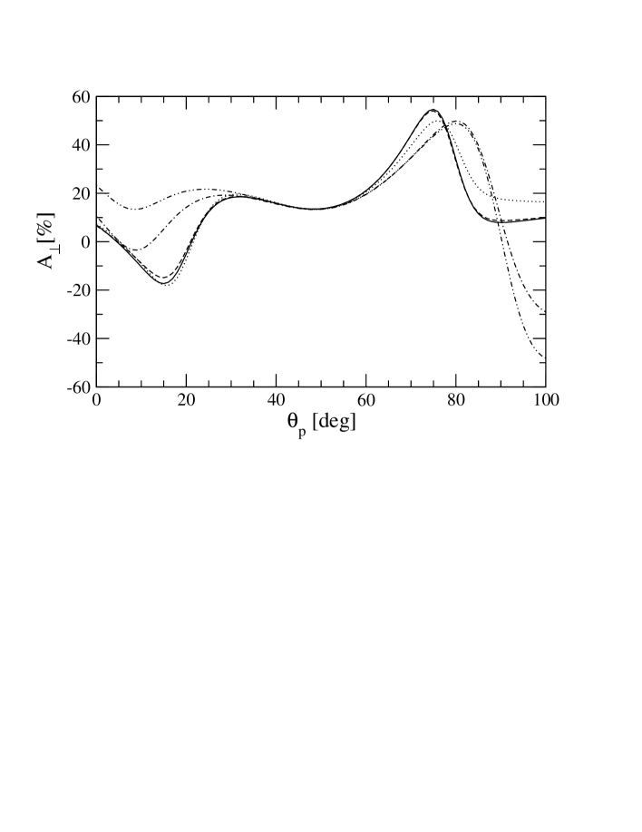
Figure 3: The perpendicular helicity asymmetry $A_{\perp}$ for the configuration from Table 1. Curves as in Fig. 1.

For $A_{\parallel}$ the 3N force effects are much smaller (below 1 % for strictly parallel kinematics). FSI are still visible and slightly reduce the value of $A_{\parallel}$ in relation to the PWIA result for parallel kinematics (by nearly 6 %).

The least sensitivity to the different dynamical ingredients is observed for $A_{\perp}$. In Fig. 3 we see that in a certain angular interval around $\theta_{Q}$ all curves overlap. That means that in this case one has direct access to important properties of ³He.

Let us now address the question how (in the given dynamical framework) different ³He wave function components contribute to $H_{0}$, $H_{2}$, $P_{1}$ and $P_{2}$. We compare in Figs. 4–6 results, for the full ³He wave function to results obtained with truncated wave functions. Besides the full results, we show curves including the dominant principal $S$-state, dropping the $D$- or the $S^{\prime}$-state contribution. The results, where only the principal $S$-state is included, and the ones with the $D$-state dropped agree rather well but differ visibly from the full prediction. The neglection of the $S^{\prime}$-state is hardly noticeable. The same is true for the $P$-state (not shown).

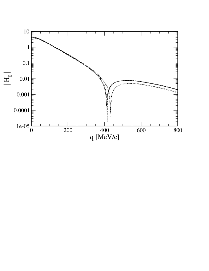
Figure 4: The quantity $H_{0}$ for different ³He states. The solid curve corresponds to the full ³He state, the dashed line shows the results for the case where the S^′ state is projected out from the full ³He state, the dotted line represents calculations where only the principal $S$-state of ³He is taken into account and finally the dash-dotted line demonstrates the effect of removing the $D$-state from the full ³He wave functions. Note that the solid and dashed lines almost completely overlap. Similarly, the dashed and dash-dotted lines are very close to each other and are slightly shifted in the zero crossing area. The lack of the $D$-waves lowers the magnitudes of $H_{0}$ at the higher $q$ values. The underlying full ³He wave function was calculated including the 3N force.

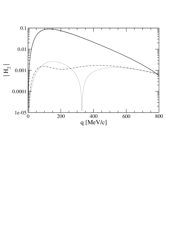
Figure 5: Curves as in Fig. 4 for the quantity $H_{2}$, which is clearly dominated by the $D$-state contributions.

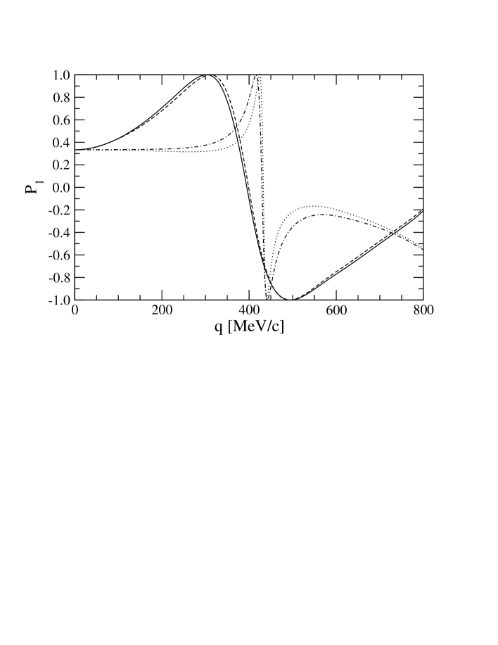
Figure 6: Curves as in Fig. 4 for the quantity $P_{1}$. The lack of $D$-wave contributions is clearly visible except for very small $q$-values.

Further we show in Fig. 7 that the 3N force effects for the quantity $P_{1}$ are rather small. The same holds for $P_{2}$ (not shown).

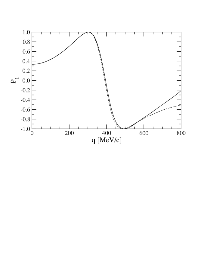
Figure 7: The quantity $P_{1}$ calculated with the inclusion of the 3N force (solid line) and without the 3N force (dashed line).

We end this section with Fig. 8, which shows the integrands $f_{1}(q)$ and $f_{2}(q)$ appearing in the second line of Eq. (40). We see that relatively small $q$ values ($q\lesssim 350$ (MeV/c) contribute to $P_{\rm int}$. The $P_{\rm int}$ value calculated with (without) the inclusion of the 3N force is -0.364 (-0.362). For completeness we give also the values of the two integrals appearing in Eq. (40): $\int\limits_{0}^{\infty}dq\,f_{1}(q)$ = 0.127 (0.128), $\int\limits_{0}^{\infty}dq\,f_{2}(q)$ = 0.348 (0.354) when calculated with (without) the 3N force. The latter integral gives up to the factor $\pi/4$ the probability to find a proton-deuteron cluster inside ³He.

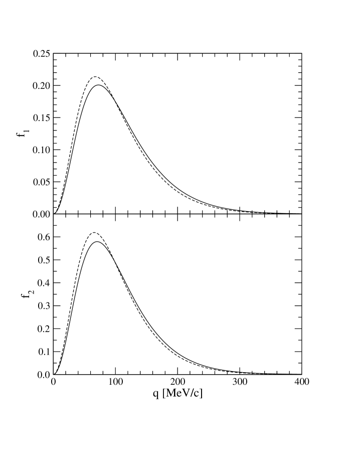
Figure 8: The integrands $f_{1}(q)$ (left) and $f_{2}(q)$ (right) appearing in Eq. (40). Curves as in Fig. 7.

IV Results for the $\vec{{}^{3}{\rm He}}({\vec{e}},e^{\prime}p)pn$ and $\vec{{}^{3}{\rm He}}({\vec{e}},e^{\prime}n)pp$ processes

In this section the results for the three-body breakup will be discussed. A general discussion would require that all the elements of our dynamical framework are involved, i.e. that the initial ³He and final scattering states are calculated consistently and many-body currents are taken into account. We refer the reader to report for a discussion of the numerical techniques necessary to perform calculations for such an approach. It, however, precludes any analytical insight. Thus, as for the $\vec{{}^{3}{\rm He}}({\vec{e}},e^{\prime}p)d$ process, we start with the PWIA approximation. Additionally, we restrict the full ³He state to its main, principal $S$-state component. In this case the six nonrelativistic response functions $W_{i}$ for the exclusive $\vec{{}^{3}{\rm He}}({\vec{e}},e^{\prime}p)pn$ reaction take especially simple forms

$$W_{L}=\frac{4\,{\,{G_{E}^{p}}}^{2}\,H^{2}}{6}$$ (43)

$$W_{T}=\frac{2\,H^{2}\,\left({\,{G_{M}^{p}}}^{2}\,{\,{Q}}^{2}+{\,{G_{E}^{p}}}^{2}\,{\,{q_{f}}}^{2}-{\,{G_{E}^{p}}}^{2}\,{\,{q_{f}}}^{2}\,\cos(2\,\,{\theta_{1}})\right)}{6\,{\,{M}}^{2}}$$ (44)

$$W_{TT}=\frac{-4\,{\,{G_{E}^{p}}}^{2}\,H^{2}\,{\,{q_{f}}}^{2}\,\cos(2\,\,{\phi_{1}})\,{\sin^{2}(\,{\theta_{1}})}}{6\,{\,{M}}^{2}}$$ (45)

$$W_{TL}=\frac{8\,{\sqrt{2}}\,{\,{G_{E}^{p}}}^{2}\,H^{2}\,\,{q_{f}}\,\cos(\,{\phi_{1}})\,\sin(\,{\theta_{1}})}{6\,\,{M}}$$ (46)

$$W_{T^{\prime}}=0$$ (47)

$$W_{{TL}^{\prime}}=0$$ (48)

As before, $\theta_{1}$ and $\phi_{1}$ are the polar and azimuthal angles corresponding to the $\vec{q}_{f}\equiv\frac{2}{3}\left[\vec{p}_{1}-\frac{1}{2}\left(\vec{p}_{2}+\vec{p}_{3}\right)\right]={\vec{p}}_{p}-\frac{1}{3}{\vec{Q}}$ direction. The quantity $H$ is defined as

$$H\,=\,\Psi^{\rm PSS}\left(\vec{p}_{f},\vec{q}_{f}-\frac{2}{3}\vec{Q}\,\right),$$ (49)

where $\vec{p}_{f}$ is the Jacobi momentum describing the relative motion within the $23$ (proton-neutron) pair:

$$\vec{p}_{f}=\frac{1}{2}\left(\vec{p}_{2}-\vec{p}_{3}\right).$$ (50)

The individual final nucleon momenta are denoted by $\vec{p}_{1}$, $\vec{p}_{2}$ and $\vec{p}_{3}$ and the proton, to which the virtual photon is coupled, is the nucleon 1. The wave function $\Psi^{\rm PSS}\left(\vec{p},\vec{q}\,\right)$ is the momentum part of the principal $S$-state:

$$\mid\Psi^{\rm PSS}\rangle\equiv\int d^{3}p\,\int d^{3}q\,\mid\vec{p}\,\rangle\,\mid\vec{q}\,\rangle\,\Psi^{\rm PSS}\left(\vec{p},\vec{q}\,\right)\,\mid\zeta_{a}\,\rangle,$$ (51)

where $\mid\zeta_{a}\,\rangle$ is the completely anti-symmetric 3N spin-isospin state.

The vanishing of the $W_{{T}^{\prime}}$ and $W_{{TL}^{\prime}}$ response functions reflects the well known fact that for the principal $S$-state the proton in ³He is totally unpolarized.

The situation for the case where the photon ejects the neutron is quite different and corresponds very closely to electron scattering on a free, fully polarized neutron at rest. The six nonrelativistic response functions $W_{i}$ for the exclusive $\vec{{}^{3}{\rm He}}({\vec{e}},e^{\prime}n)pp$ reaction under the PWIA approximation and assuming only the principal S-state in the ³He wave function can be written in the laboratory frame as

$$W_{L}=\frac{2\,{\,{G_{E}^{n}}}^{2}\,H^{2}}{6}$$ (52)

$$W_{T}=\frac{H^{2}\,\left({\,{G_{M}^{n}}}^{2}\,{\,{Q}}^{2}+{\,{G_{E}^{n}}}^{2}\,{\,{q_{f}}}^{2}-{\,{G_{E}^{n}}}^{2}\,{\,{q_{f}}}^{2}\,\cos(2\,\,{\theta_{1}})\right)}{6\,{\,{M}}^{2}}$$ (53)

$$W_{TT}=\frac{-2\,{\,{G_{E}^{n}}}^{2}\,H^{2}\,{\,{q_{f}}}^{2}\,\cos(2\,\,{\phi_{1}})\,{\sin^{2}(\,{\theta_{1}})}}{6\,{\,{M}}^{2}}$$ (54)

$$W_{TL}=\frac{4\,{\sqrt{2}}\,{\,{G_{E}^{n}}}^{2}\,H^{2}\,\,{q_{f}}\,\cos(\,{\phi_{1}})\,\sin(\,{\theta_{1}})}{6\,\,{M}}$$ (55)

$$W_{T^{\prime}}=\frac{-{G_{M}^{n}}\,H^{2}\,\,{Q}\,\left(\,{G_{M}^{n}}\,\,{Q}\,\cos(\,{\theta^{\star}})-2\,\,{G_{E}^{n}}\,\,{q_{f}}\,\cos(\,{\phi_{1}}-\,{\phi^{\star}})\,\sin(\,{\theta_{1}})\,\sin(\,{\theta^{\star}})\right)}{6\,{\,{M}}^{2}}$$ (56)

$$W_{{TL}^{\prime}}=\frac{2\,{\sqrt{2}}\,\,{G_{E}^{n}}\,\,{G_{M}^{n}}\,H^{2}\,\,{Q}\,\cos(\,{\phi^{\star}})\,\sin(\,{\theta^{\star}})}{6\,\,{M}}$$ (57)

Now the $\theta_{1}$ and $\phi_{1}$ angles correspond to the $\vec{q}_{f}={\vec{p}}_{1}-\frac{1}{3}{\vec{Q}}\equiv{\vec{p}}_{n}-\frac{1}{3}{\vec{Q}}$ direction and $\vec{p}_{f}$ is the Jacobi momentum describing the relative motion within the $23$ proton-proton pair.

Let us first illustrate the influence of different ³He wave function components on the asymmetries $A_{\parallel}$ and $A_{\perp}$ performing calculations that take various components of the ³He wave function into account. This is done in Figs. 9 and 10 for the $\vec{{}^{3}{\rm He}}({\vec{e}},e^{\prime}p)np$ reaction. We note that the formulas (43)–(48) and (52)–(57) apply also to the semi-exclusive reaction. One has to make a simple replacement

$$H^{2}\longrightarrow\int d\,{\hat{p}}_{f}\,H^{2},$$ (58)

i.e., to integrate over the unobserved direction of the relative momentum within the $23$ pair.

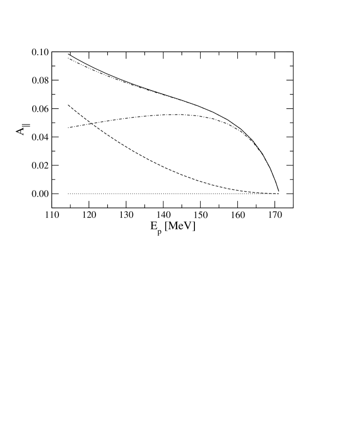
Figure 9: The parallel asymmetry $A_{\parallel}$ for the proton ejection in the virtual photon direction as a function of the emitted proton energy $E_{p}$ for the electron configuration from Table 1 for different ³He states. Curves as in Fig. 4 except that the additional double-dot-dashed line demonstrates the effect of removing the $P$-state from the full ³He wave function.

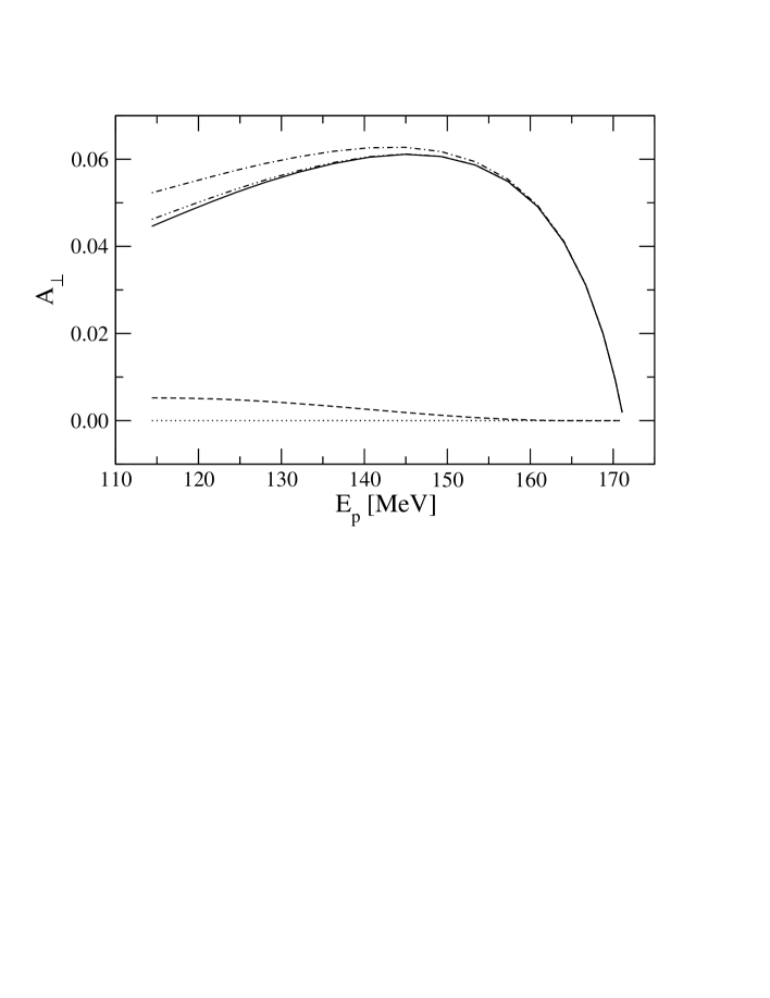
Figure 10: The same as in Fig. 9 for the perpendicular asymmetry $A_{\perp}$.

We see that both asymmetries change quite significantly in the given $E_{p}$ range and become very small for the largest $E_{p}$ values. For the principal $S$-state alone both asymmetries are zero. Therefore the smaller ³He components (except the $P$-wave) are significant in PWIA and change the asymmetry in the proton case. Thereby the $S^{\prime}$-contribution is more important than the $D$-wave piece.

The situation is quite different for the neutron knock-out asymmetries shown in Figs. 11 and 12. In this case the asymmetries are non-zero even for the principal $S$-state wave function.

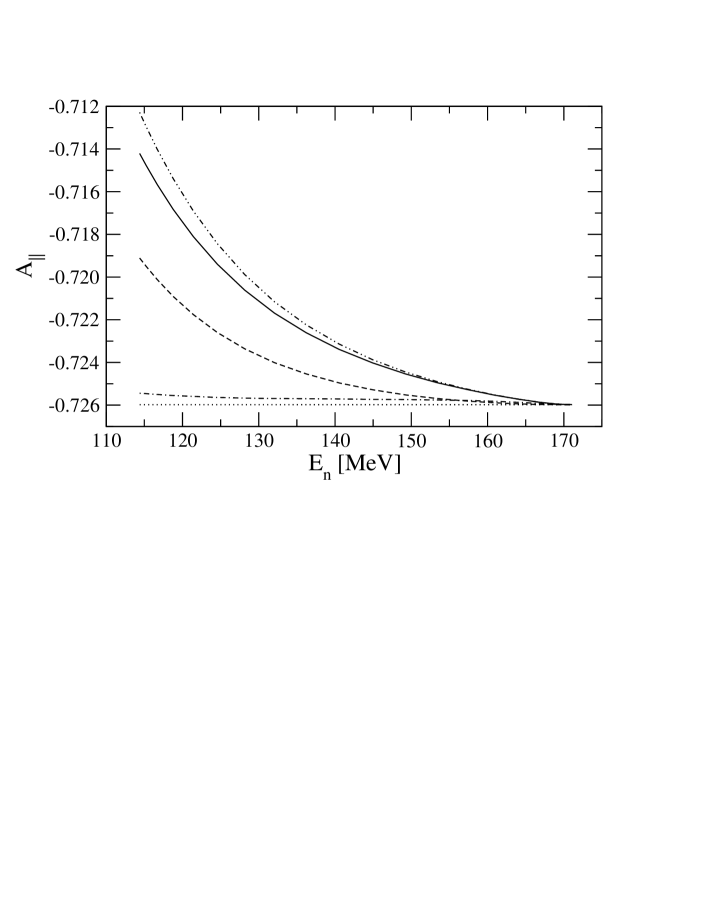
Figure 11: The same as in Fig. 9 for the neutron knock-out.

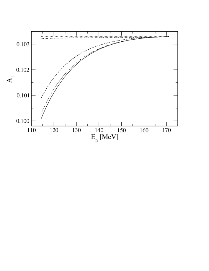
Figure 12: The same as in Fig. 10 for the neutron knock-out.

All results are quite stable in the shown $E_{n}$ range. The change due to different ³He states for $A_{\parallel}$ amounts to 2 % and $A_{\perp}$ varies by $\approx$ 3 %. The asymmetries reach the specific values which depend only on the neutron electromagnetic form factors and trivial kinematic factors $v_{i}$ appearing in Eq. (5).

The PWIA picture is very simple but quite unrealistic. That is why FSI has to be taken into account. In order to retain analytical insight but make our framework more realistic we will in the following additionally allow for the rescattering effects in the subsystem $23$ and call the resulting approximation $FSI23$. The ³He wave function will still be restricted to the principal $S$-state. Thus we need the following matrix elements $N^{\mu}$ of the single nucleon current $j_{1}^{\nu}({\vec{Q}})$ (see report for more details of our notation)

$$N^{\mu}=\langle\,{\vec{p}}_{1}\,{\vec{p}}_{23}\,{\vec{p}}_{f}\,sm_{s}\,\frac{1}{2}m_{1};tm_{t}\,\frac{1}{2}\nu_{1}\mid\left(1+t_{23}G_{0}\right)j_{1}^{\nu}({\vec{Q}})\mid\Psi^{\rm PSS}M_{S}M_{T}=\frac{1}{2}\rangle,$$ (59)

where

$${\vec{p}}_{23}\equiv{\vec{p}}_{2}+{\vec{p}}_{3},$$ (60)

the $23$ pair spin and spin projection are denoted by $s$ and $m_{s}$, the $23$ pair isospin and isospin projection are $t$ and $m_{t}$ and the spin and isospin magnetic quantum numbers of the nucleon 1 are $m_{1}$ and $\nu_{1}$. The total ³He spin and isospin projections are $M_{S}$ and $M_{T}$, respectively. Further $t_{23}$ is the NN $t$-matrix acting within the $23$ pair and $G_{0}$ is the free 3N propagator.

The six nonrelativistic response functions $W_{i}$ for the exclusive $\vec{{}^{3}{\rm He}}({\vec{e}},e^{\prime}p)pn$ reaction under the FSI23 approximation and assuming only the principal S-state in the ³He wave function can be written in the laboratory frame as

$$W_{L}=\frac{{G_{E}^{p}}^{2}\,H_{1}}{6}$$ (61)

$$W_{T}=\frac{\left({\,{G_{M}^{p}}}^{2}\,{\,{Q}}^{2}+{\,{G_{E}^{p}}}^{2}\,{\,{q_{f}}}^{2}-{\,{G_{E}^{p}}}^{2}\,{\,{q_{f}}}^{2}\,\cos(2\,\,{\theta_{1}})\ \right)\,H_{1}\,}{12\,{\,{M}}^{2}}$$ (62)

$$W_{TT}=\frac{-{\,{G_{E}^{p}}}^{2}\,{\,{q_{f}}}^{2}\,\cos(2\,\,{\phi_{1}})\,\,{\sin^{2}(\,{\theta_{1}})}\,H_{1}\,}{6\,{\,{M}}^{2}}$$ (63)

$$W_{TL}=\frac{{\sqrt{2}}\,{\,{G_{E}^{p}}}^{2}\,\,{q_{f}}\,\cos(\,{\phi_{1}})\,\,\sin(\,{\theta_{1}})\,H_{1}\,}{3\,\,{M}}$$ (64)

$$W_{T^{\prime}} = \frac{\,-\left({G_{M}^{p}}\,{Q}\,\right)^{2}\,H_{2}\,\cos(\,{\theta^{\star}})\,}{12\,{\,{M}}^{2}}$$ (65)

$$+ \frac{\,2\,{\sqrt{2}}\,\,{G_{E}^{p}}\,{G_{M}^{p}}\,{Q}\,{q_{f}}\,H_{3}\,\cos(\,{\phi_{1}})\,\sin(\,{\theta_{1}})\,\cos(\,{\theta^{\star}})\,}{12\,{\,{M}}^{2}}$$

$$+ \frac{\,2\,{\sqrt{2}}\,\,{G_{E}^{p}}\,{G_{M}^{p}}\,{Q}\,{q_{f}}\,i\,H_{4}\,\sin(\,{\phi_{1}})\,\sin(\,{\theta_{1}})\,\cos(\,{\theta^{\star}})\,}{12\,{\,{M}}^{2}}$$

$$- \frac{\,{\sqrt{2}}\,\left({G_{M}^{p}}\,\,{Q}\,\right)^{2}\,\left(\cos(\,{\phi^{\star}})\,\,H_{3}\,+i\,H_{4}\,\sin(\,{\phi^{\star}})\right)\,\sin(\,{\theta^{\star}})}{12\,{\,{M}}^{2}}$$

$$+ \frac{\,2\,{G_{E}^{p}}\,{G_{M}^{p}}\,{Q}\,{q_{f}}\,H_{5}\,\cos(\,{\phi_{1}}+\,{\phi^{\star}})\,\sin(\,{\theta_{1}})\,\sin(\,{\theta^{\star}})}{12\,{\,{M}}^{2}}$$

$$+ \frac{\,2\,{G_{E}^{p}}\,{G_{M}^{p}}\,{Q}\,{q_{f}}\,H_{6}\,\cos(\,{\phi_{1}}-\,{\phi^{\star}})\,\sin(\,{\theta_{1}})\,\sin(\,{\theta^{\star}})}{12\,{\,{M}}^{2}}$$

$$- \frac{\,2\,{G_{E}^{p}}\,{G_{M}^{p}}\,{Q}\,{q_{f}}\,i\,H_{7}\,\sin(\,{\phi_{1}}+\,{\phi^{\star}})\,\sin(\,{\theta_{1}})\,\sin(\,{\theta^{\star}})}{12\,{\,{M}}^{2}}$$

$$W_{TL^{\prime}} = \frac{\,2\,{G_{E}^{p}}\,\,{G_{M}^{p}}\,\,{Q}\,H_{3}\,\cos(\,{\theta^{\star}})\,}{6\,\,{M}}$$ (66)

$$+ \frac{\,{\sqrt{2}}\,{G_{E}^{p}}\,\,{G_{M}^{p}}\,\,{Q}\,H_{8}\,\cos(\,{\phi^{\star}})\,\sin(\,{\theta^{\star}})\,}{6\,\,{M}}$$

$$- \frac{\,4\,{\sqrt{2}}\,{G_{E}^{p}}\,\,{G_{M}^{p}}\,\,{Q}\,H_{9}\,\sin(\,{\phi^{\star}})\,\sin(\,{\theta^{\star}})\,}{6\,\,{M}}$$

The auxiliary quantities $H_{1}$–$H_{9}$ are

$$H_{1}\ \equiv\ {\mid G(1)\mid}^{2}+2\,\left({\mid G(4)\mid}^{2}+{\mid G(5)\mid}^{2}+{\mid G(6)\mid}^{2}+{\mid G(7)\mid}^{2}\right)+{G(8)}^{2}$$ (67)

$$H_{2}\ \equiv\ {\mid G(1)\mid}^{2}-2\,\left({\mid G(4)\mid}^{2}-{\mid G(5)\mid}^{2}+{\mid G(6)\mid}^{2}+{\mid G(7)\mid}^{2}\right)+{G(8)}^{2}$$ (68)

$$H_{3}\ \equiv\ \left((G(4))^{\star}-(G(6))^{\star}\right)\,G(5)+(G(5))^{\star}\,\left(G(4)-G(6)\right)+2\,G(8)\,\Re{G(7)}$$ (69)

$$H_{4}\ \equiv\ -\left(\left((G(4))^{\star}+(G(6))^{\star}\right)\,G(5)\ \right)+(G(5))^{\star}\,\left(G(4)+G(6)\right)+2\,i\,G(8)\,\Im{G(7)}$$ (70)

$$H_{5}\ \equiv\ {(G(7))^{\star}}^{2}-2\,(G(6))^{\star}\,G(4)-2\,(G(4))^{\star}\,G(6)+{G(7)}^{2}$$ (71)

$$H_{6}\ \equiv\ {\mid G(1)\mid}^{2}-2\,{\mid G(5)\mid}^{2}-{G(8)}^{2}$$ (72)

$$H_{7}\ \equiv\ {(G(7))^{\star}}^{2}+2\,(G(6))^{\star}\,G(4)-2\,(G(4))^{\star}\,G(6)-{G(7)}^{2}$$ (73)

$$H_{8}\ \equiv\ {\mid G(1)\mid}^{2}-2\,{\mid G(5)\mid}^{2}+{(G(7))^{\star}}^{2}$$

$$-2\,(G(6))^{\star}\,G(4)-2\,(G(4))^{\star}\,G(6)+{G(7)}^{2}-{G(8)}^{2}\$$ (74)

$$H_{9}\ \equiv\ \Im{G(6)}\,\Re{G(4)}-\Im{G(4)}\,\Re{G(6)}+\Im{G(7)}\,\Re{G(7)}$$ (75)

The different $G(i)$ functions that appear in the equations are the integrals

$$F(s,m_{s},m_{s^{\prime}},t,m_{t})\ \equiv\ \int d{\vec{p}}^{\,\prime}\,\langle{\vec{p}}_{f}\,sm_{s}\,tm_{t}\mid 1+t_{23}G_{0}\mid{\vec{p}}^{\,\prime}\,sm_{s^{\prime}}\,tm_{t}\rangle\,\Psi^{\rm PSS}\left({\vec{p}}^{\,\prime},\vec{q}_{f}-\frac{2}{3}\vec{Q}\,\right)$$ (76)

for different combinations of $s$, $m_{s}$, $m_{s^{\prime}}$, $t$ and $m_{t}$:

$$G(1)=F(0,0,0,1,0)$$

$$G(2)=F(0,0,0,1,1)$$

$$G(3)=F(0,0,0,1,-1)$$

$$G(4)=F(1,-1,-1,0,0)$$

$$G(5)=F(1,-1,0,0,0)$$

$$G(6)=F(1,-1,1,0,0)$$

$$G(7)=F(1,0,-1,0,0)$$

$$G(8)=F(1,0,0,0,0)$$

$$G(9)=F(1,0,1,0,0)$$

$$G(10)=F(1,1,-1,0,0)$$

$$G(11)=F(1,1,0,0,0)$$

$$G(12)=F(1,1,1,0,0)$$ (77)

In the case of ³He $G(3)$ is absent.

Due to the assumed $t$-matrix properties (isospin invariance and invariance with respect to time reversal)

$$G(3)=G(2)=G(1)$$

$$G(10)=\left(G(6)\right)^{\star}$$

$$G(9)=-\left(G(7)\right)^{\star}$$

$$G(12)=\left(G(4)\right)^{\star}$$

$$G(11)=-\left(G(5)\right)^{\star}$$

$$G(8)=\left(G(8)\right)^{\star}$$ (78)

some of the combinations could be eliminated. When the term $t_{23}G_{0}$ in Eq. (76) is dropped then

$$F(s,m_{s},m_{s^{\prime}},t,m_{t})=\delta_{m_{s},m_{s^{\prime}}}\,,$$ (79)

the quantities $H_{2}$–$H_{9}$ vanish and $H_{1}$ reduces to $4\left(G(1)\right)^{2}$. In this way the PWIA results of Eqs. (43)–(48) are recovered.

For the sake of completeness we give also the corresponding (and much simpler) expressions for the six nonrelativistic response functions $W_{i}$ in the case of the exclusive $\vec{{}^{3}{\rm He}}({\vec{e}},e^{\prime}n)pp$ reaction under the same dynamical assumptions:

$$W_{L}=\frac{{\,{G_{E}^{n}}}^{2}\,{\mid G(2)\mid}^{2}}{3}$$ (80)

$$W_{T}=\frac{{\mid G(2)\mid}^{2}\,\left({\,{G_{M}^{n}}}^{2}\,{\,{Q}}^{2}+{\,{G_{E}^{n}}}^{2}\,{\,{q_{f}}}^{2}-{\,{G_{E}^{n}}}^{2}\,{\,{q_{f}}}^{2}\,\cos(2\,\,{\theta_{1}})\ \right)}{6\,{\,{M}}^{2}}$$ (81)

$$W_{TT}=\frac{-{\mid G(2)\mid}^{2}\,{\,{G_{E}^{n}}}^{2}\,{\,{q_{f}}}^{2}\,\cos(2\,\,{\phi_{1}})\,{\sin^{2}(\,{\theta_{1}})}}{3\,{\,{M}}^{2}}$$ (82)

$$W_{TL}=\frac{2\,{\sqrt{2}}\,{\,{G_{E}^{n}}}^{2}\,\,{q_{f}}\,{\mid G(2)\mid}^{2}\,\cos(\,{\phi_{1}})\,\sin(\,{\theta_{1}})}{3\,\,{M}}$$ (83)

$$W_{T^{\prime}}=\frac{-{G_{M}^{n}}\,\,{Q}\,{\mid G(2)\mid}^{2}\,\left(\,{G_{M}^{n}}\,\,{Q}\,\cos(\,{\theta^{\star}})-2\,\,{G_{E}^{n}}\,\,{q_{f}}\,\cos({\phi_{1}}-\,{\phi^{\star}})\,\sin({\theta_{1}})\,\sin({\theta^{\star}})\,\right)}{6\,{\,{M}}^{2}}$$ (84)

$$W_{TL^{\prime}}=\frac{{\sqrt{2}}\,\,{G_{E}^{n}}\,\,{G_{M}^{n}}\,\,{Q}\,{\mid G(2)\mid}^{2}\,\cos(\,{\phi^{\star}})\,\sin(\,{\theta^{\star}})}{3\,\,{M}}$$ (85)

The response functions have the same form as for the PWIA approximation displayed in Eqs. (52)–(57). The simple form of Eqs. (80)–(85) is guaranteed by the fact that for the neutron emission only $t$-matrices with the total subsystem isospin $t=1$ contribute. If one forms now the helicity asymmetries $A(\theta^{\star}\,,\,\phi^{\star}\,)$, then exactly the same form is obtained as in the case of PWIA, i.e., all information from ³He (restricted to the principal $S$-state) disappears.

The formula (59) and the following $t$-matrices are given in the three-vector representation. Since we work with partial wave decomposed $t$-matrices, it is adequate to ask the question if the interaction is dominated by one or very few channel states. Further we would like to see if the truncation of the ³He wave function to the principal $S$-state is reasonable, at least for the highest energies of the emitted nucleon.

Let us start with the more intricate case of the proton emission. In Figs. 13 and 14 we show different curves obtained with the full ³He state (thick lines) and with ³He truncated to the principal $S$-state (thin lines) for different number of $t$-matrix partial waves.

Figure 13: The parallel asymmetry $A_{\parallel}$ for the proton ejection in the virtual photon direction as a function of the ejected proton energy $E_{p}$ for the electron configuration from Table 1 under the $FSI23$ approximation. Dash-dotted lines are obtained for the case, where the $t$-matrix acts only in the ${}^{1}S_{0}$ channel, dashed lines correspond to the calculations in which only the ${}^{1}S_{0}$ and ${}^{3}S_{1}$ $t$-matrix components are taken into account (without coupling to the ${}^{3}D_{1}$ state), dotted lines show the results for ${}^{1}S_{0}$ and ${}^{3}S_{1}$–${}^{3}D_{1}$ states and finally solid lines correspond to inclusion of all nucleon-nucleon $t$-matrix partial waves with the total angular momentum $j\leq 3$. Thick lines are obtained with the full ³He state and thin lines with ³He truncated to the principal $S$-state. Note that the thin dotted and solid lines completely overlap.

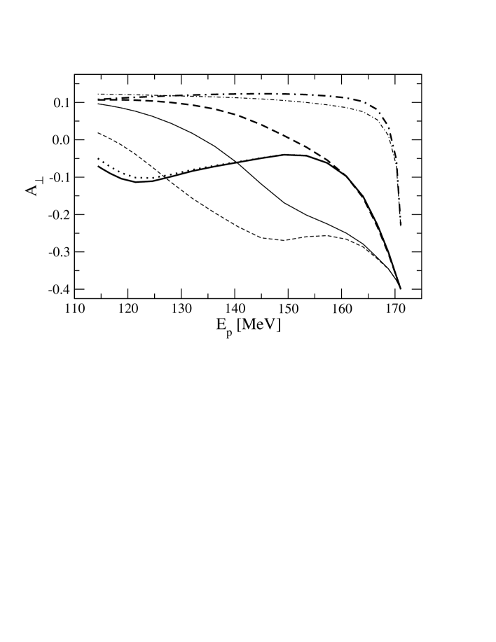
Figure 14: The same as in Fig. 13 for the perpendicular asymmetry $A_{\perp}$.

We note first of all that both cases of the parallel and perpendicular asymmetries are quite similar, especially for the range of the asymmetry values. It is clear that the truncation of the full ³He wave function to the principal $S$-state is valid only for the highest emission energies. Otherwise the influence of the smaller ³He wave function components is very strong. Another important observation is that even for these highest energies the action of the $t$-matrix cannot be restricted to just one ${}^{1}S_{0}$ channel and the inclusion at least of the ${}^{3}S_{1}$ partial wave state is inevitable. Since then both spins $s=0$ and $s=1$ appear for the $np$ subsystem, the photon couples to the proton which is polarized along and opposite to the spin of polarized ³He. If in the $np$ subsystem only the spin $s=0$ were active, the photon would couple to the 100 % polarized proton.

The situation for the neutron emission shown in Figs. 15 and 16 is much simpler and we do not observe so much sensitivity to different dynamical components. The $t$-matrix is anyway forced to act in the total isospin $t=1$ states. Since additionally for the highest neutron energies (the lowest subsystem $23$ energies) the nucleon-nucleon interaction is restricted to $s$-waves, that implies that only the ${}^{1}S_{0}$ partial wave should be important. This expectation is confirmed by our results.

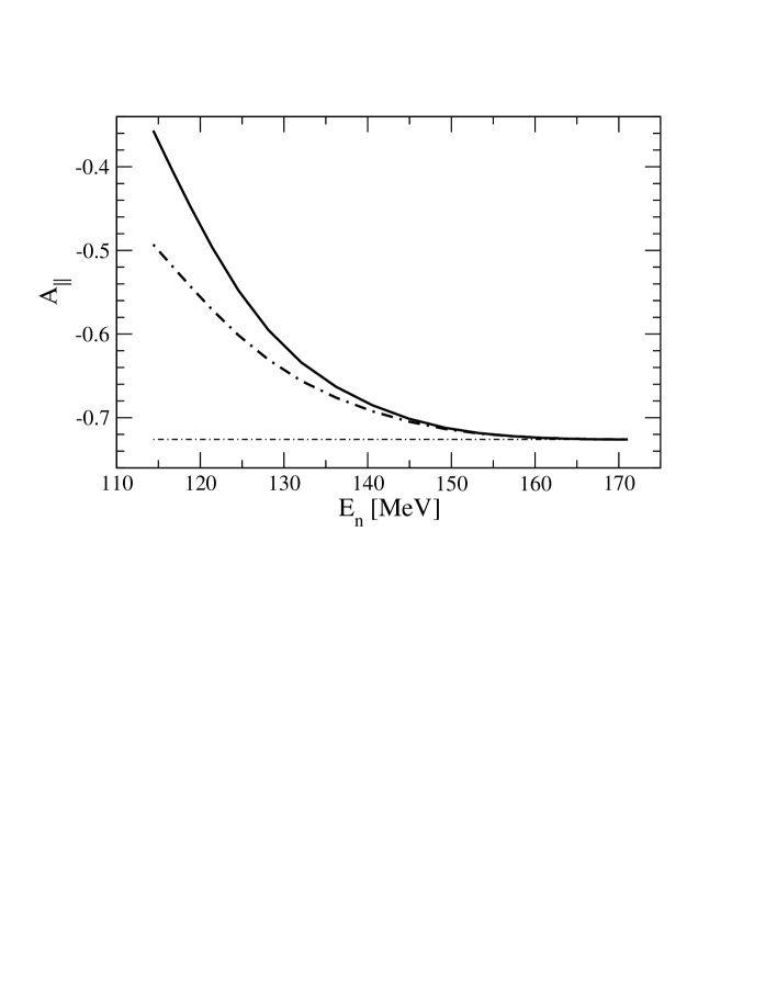
Figure 15: The parallel asymmetry $A_{\parallel}$ for the neutron emission in the virtual photon direction as a function of the ejected neutron energy $E_{n}$ for the electron configuration from Table 1 under the $FSI23$ approximation. Since in this case only $t=1$ states contribute to the $t_{23}G_{0}$ part of the $FSI23$ matrix elements, we show only three cases: the results obtained with the principal $S$-state and the $t$-matrix restricted to the ${}^{1}S_{0}$ state (thin dash-dotted line), the results obtained with the full ³He wave function and the $t$-matrix restricted to the ${}^{1}S_{0}$ state (thick dash-dotted line), and finally the results obtained with the full ³He wave function and the $t$-matrix acting in all partial waves with the total angular momentum $j\leq 3$ (thick solid line).

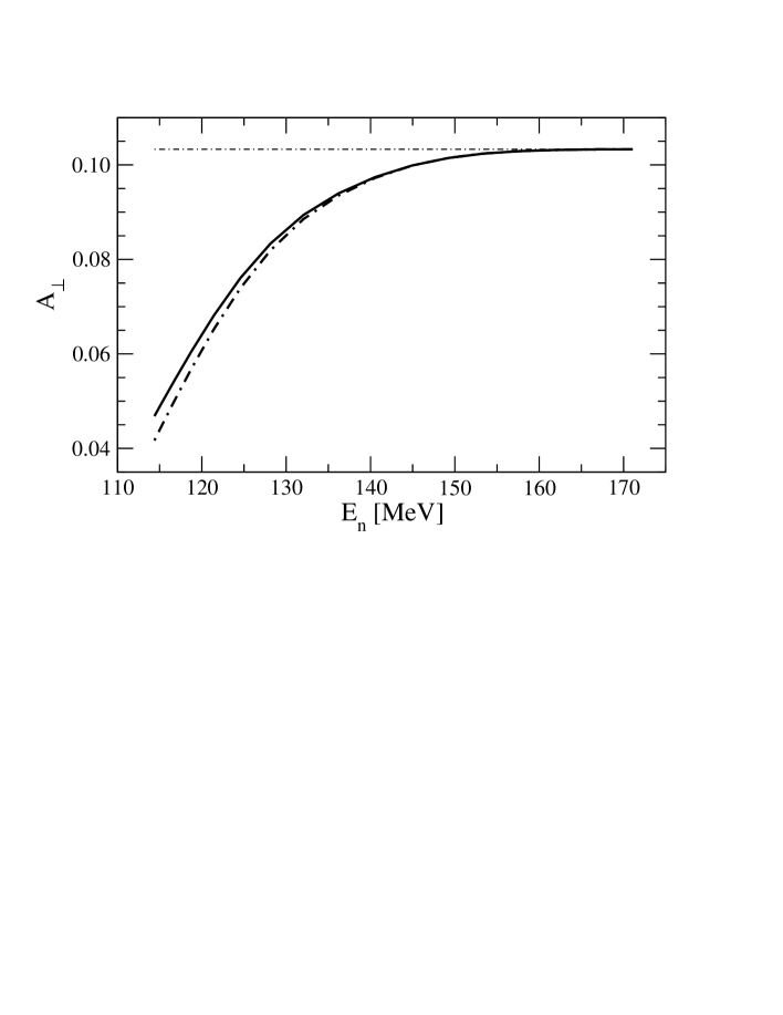
Figure 16: The same as in Fig. 15 for the perpendicular asymmetry $A_{\perp}$.

In the group of figures 17–20 we demonstrate results for much more complicated dynamical frameworks. We show first the results based on the full treatment of FSI. Then we add to our single nucleon current the $\pi$- and $\rho$-like meson exchange currents. Finally we show the results where on top of all that the UrbanaIX 3N force is present both for the initial ³He bound state and for the final scattering states. For proton emission the $FSI23$ approximation but taking the full ³He state into consideration turns out to be satisfactory at the upper end of the energy spectrum. This is valid for the both asymmetries. In the case of neutron emission the situation is different and the full dynamics, especially for $A_{\perp}$ is required. It is only in the case of $A_{\parallel}$ that at the highest neutron energies all curves coincide.

As pointed out before spindep ; Groningen04 that means that the extraction of $G_{M}^{n}$ from a measurement of the parallel asymmetry $A_{\parallel}$ seems to be quite model independent. This is not the case for the extraction of $G_{E}^{n}$ from a measurement of the perpendicular asymmetry $A_{\perp}$, which shows more sensitivity to different dynamical ingredients (see Fig 20). To minimize the effects from complicated dynamics, measurements are performed on top of the quasi-elastic peak. Since the cross section drops very fast for the neutron energies below the maximal one (see Fig 22), $A_{\perp}$ receives main contributions from the regions where the model dependence is somewhat reduced.

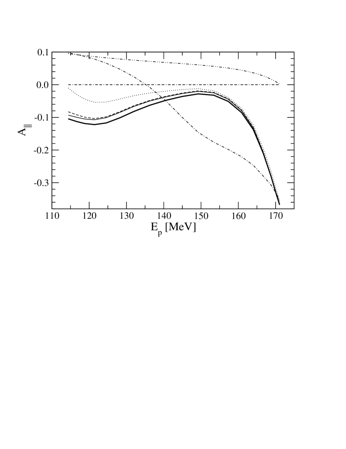
Figure 17: The parallel asymmetry $A_{\parallel}$ for the proton ejection in the virtual photon direction as a function of the ejected proton energy $E_{p}$ for the electron configuration from Table 1 under different dynamical treatments of FSI. The double-dashed-dot line shows the PWIA prediction with the principal $S$-state and the double-dotted-dash line the PWIA prediction with full ³He. Further we show again the $FSI23$ predictions with the ³He restricted to the principal $S$-state (dash-dotted line) and full ³He (dotted line). Results with the full inclusion of FSI and no MEC are plotted with the dashed line. The thin solid line represents the predictions which include the $\pi$- and $\rho$-like MEC and finally the thick solid line shows our best calculations involving in addition the UrbanaIX 3N force.

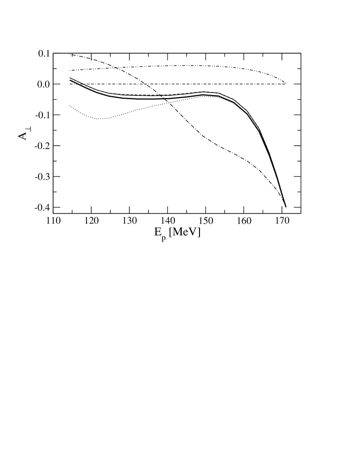
Figure 18: The same as in Fig. 17 for the perpendicular asymmetry $A_{\perp}$.

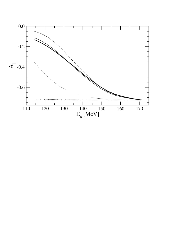
Figure 19: The same as in Fig. 17 for the neutron knock-out.

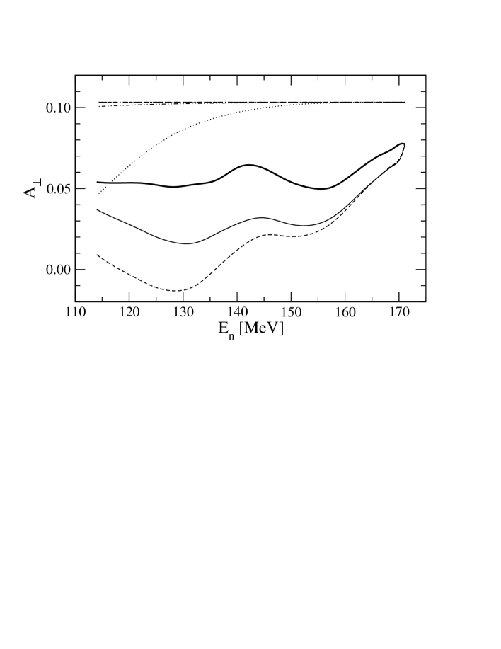
Figure 20: The same as in Fig. 19 for the perpendicular asymmetry $A_{\perp}$.

Finally in Figs. 21 and 22 we show for the sake of completeness our predictions for the six fold differential cross sections both for the proton and neutron knock-out processes.

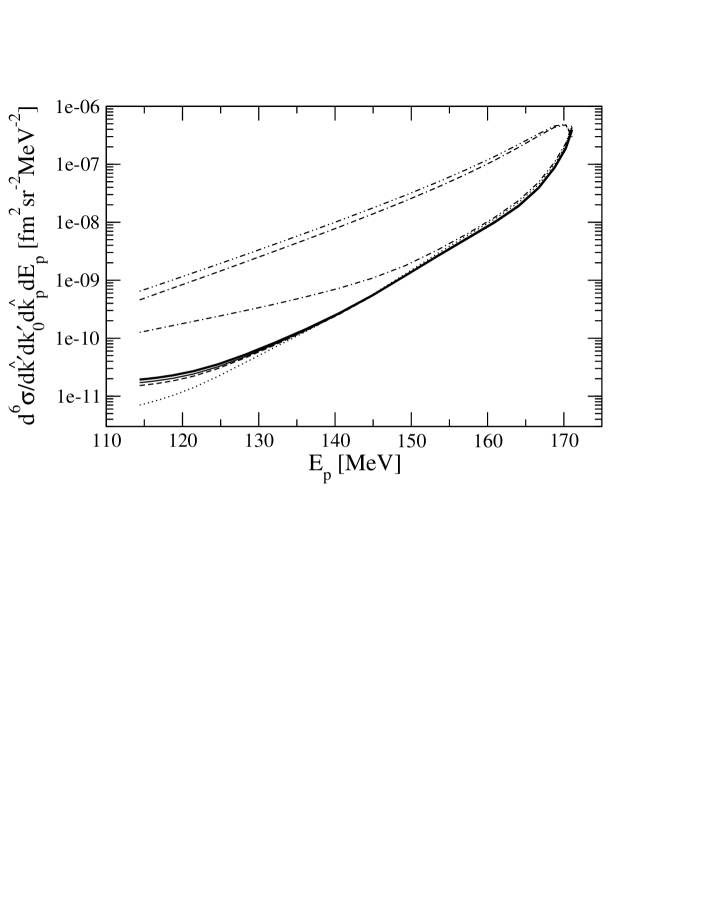
Figure 21: The six fold differential cross section for the proton ejection in the virtual photon direction as a function of the ejected proton energy $E_{p}$ for the electron configuration from Table 1 under different dynamical treatments of FSI. Curves as in Fig. 17.

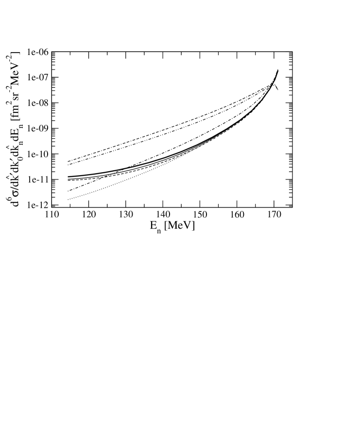
Figure 22: The same as in Fig. 21 for the neutron knock-out process.

V Summary

The present paper is motivated by a recent experiment Achenbach05 , where for the first time the $A_{\parallel}$ and $A_{\perp}$ asymmetries were measured for proton emission in the two- and three-body breakup of ³He. We present results for one of the electron kinematics measured in  Achenbach05 . For the $\vec{{}^{3}{\rm He}}({\vec{e}},e^{\prime}p)d$ process this paper is a continuation of work in spindep , where the spin dependent momentum distributions of proton-deuteron clusters in polarized ³He were investigated. Thus we can confirm that choosing the so-called parallel kinematics and small final deuteron momenta, information about proton polarization in ³He is directly available. We found that in such a case the polarizations extracted from the parallel and perpendicular asymmetries are not independent but simply related. This relation has been to some extent confirmed in  Achenbach05 . For these specific kinematical conditions FSI (including the 3N force effects) and MEC do not play a big role and the PWIA picture is sufficient. One should exploit this opportunity and obtain all possible information about ³He. On the other hand, this could also be a method to measure the proton electromagnetic form factors, even though they are known from direct electron scattering on a proton target. Such a measurement on ³He would verify our knowledge about this nucleus and help set a limit on medium corrections of the form factors.

The situation for the $\vec{{}^{3}{\rm He}}({\vec{e}},e^{\prime}p)pn$ reaction is more complicated since the simplest PWIA approximation is not valid. For the proton emission we find a lot of sensitivity to the smaller ³He wave function components because for the main principal $S$-state of ³He the asymmetries are zero. FSI has to be taken into account but for the parallel kinematics and high emitted proton energies it can be approximated by a simpler $FSI23$ prescription. This is in agreement with the results of a study performed in spectral . We find, however, that no picture of electron scattering on a polarized proton arises. The reason is that even at the highest proton energies partial waves with spin $s=0$ and $s=1$ contribute.

For the $\vec{{}^{3}{\rm He}}({\vec{e}},e^{\prime}n)pp$ reaction we see again (see sensitivity ) different sensitivities of the $A_{\parallel}$ and $A_{\perp}$ asymmetries to the dynamical ingredients of our Faddeev framework. This proves that the extraction of $G_{M}^{n}$ from a measurement of the parallel asymmetry $A_{\parallel}$ would be very simple. This is not quite the case for the extraction of $G_{E}^{n}$ from a measurement of the perpendicular asymmetry $A_{\perp}$, where corrections from FSI, MEC and 3N forces would play a more important role. The theoretical uncertainties can be, however, minimized by a proper choice of experimental conditions.

Finally, we would like to emphasize that the results reflect our present day understanding of the reaction mechanism and the structure of ³He. Therefore new data for the processes addressed in this paper would be extremely useful.

References

(1) J. L. Forest, V. R. Pandharipande, Steven C. Pieper,
R. B. Wiringa, R. Schiavilla, A. Arriaga,
Phys. Rev. C54, 646 (1996).
(2) J. Golak, W. Glöckle, H. Kamada, H. Witała,
R. Skibiński, A. Nogga,
Phys. Rev. C65, 064004 (2002).
(3) P. Achenbach et al., nucl-ex/0505012.
(4) W. Glöckle, The Quantum Mechanical
Few-Body Problem (Springer-Verlag, Berlin, 1983).
(5) T. W. Donnelly, A. S. Raskin, Ann. Phys. (N.Y.) 169, 247 (1986).
(6) J. Golak, R. Skibiński, H. Witała, W. Glöckle,
A. Nogga, H. Kamada, Phys. Rep. 415, 89 (2005).
(7) R. B. Wiringa, V.G.J. Stoks, R. Schiavilla,
Phys. Rev. C51, 38 (1995).
(8) B. S. Pudliner, V. R. Pandharipande,
J. Carlson, Steven C. Pieper and R. B. Wiringa,
Phys. Rev. C56, 1720 (1997).
(9) D. O. Riska, Phys. Scr. 31, 107 (1985);
D. O. Riska, Phys. Scr. 31, 471 (1985).
(10) J. Golak, R. Skibiński, H. Witała, W. Glöckle,
A. Nogga, H. Kamada,
in: N. Kalantar-Nayestenaki, R.G.E. Timmermans, B.L.G. Bakker (Eds.),
Few-Body Problems in Physics, AIP Conference Proceedings No. 768,
AIP, Melville, NY, 2005, p. 91.
(11) J. Golak, H. Witała, R. Skibiński, W. Glöckle, A. Nogga, H. Kamada,
Phys. Rev. C70, 034005 (2004).
(12) J. Golak, W. Glöckle, H. Kamada, H. Witała, R. Skibiński, A. Nogga,
Phys. Rev. C65, 044002 (2002).