Shell Model Monte Carlo method in the $pn$-formalism
and applications to the Zr and Mo isotopes

Abstract

We report on the development of a new shell-model Monte Carlo algorithm which uses the proton-neutron formalism. Shell model Monte Carlo methods, within the isospin formulation, have been successfully used in large-scale shell-model calculations. Motivation for this work is to extend the feasibility of these methods to shell-model studies involving non-identical proton and neutron valence spaces. We show the viability of the new approach with some test results. Finally, we use a realistic nucleon-nucleon interaction in the model space described by $(1p_{1/2},0g_{9/2})$ proton and $(1d_{5/2},2s_{1/2},1d_{3/2},0g_{7/2},0h_{11/2})$ neutron orbitals above the ${}^{88}\mathrm{Sr}$ core to calculate ground-state energies, binding energies, $B(E2)$ strengths, and to study pairing properties of the even-even ${}^{90-104}\mathrm{Zr}$ and ${}^{92-106}\mathrm{Mo}$ isotope chains.

I Introduction and Motivation

The Shell model Monte Carlo (SMMC) method Koonin et al. (1997a, b); Lang et al. (1993) was developed as an alternative to direct diagonalization in order to study low-energy nuclear properties. It was successfully applied to nuclear problems where large model spaces made diagonalization impractical. In the canonical SMMC approach, one calculates the thermal expectation values of observables of few-body operators by representing the imaginary-time many-body evolution operator as a superposition of one-body propagators in fluctuating auxiliary fields. Thus, one recasts the Hamiltonian diagonalization problem as a stochastic integration problem.

In this paper, we report on the development of an SMMC approach in the $pn$-formalism. This implementation of SMMC enables one to treat shell-model Hamiltonians that are not isospin invariant in the model space, or for which different model spaces are used for protons and neutrons. In the following, we will use the abbreviated form SMMCpn, to distinguish the approach discussed here from the original one. We note that special features of the pairing+quadrupole interaction enabled a special implementation of SMMC in non-degenerate proton and neutron model spaces for calculations in rare earth nuclei Dean et al. (1993); White et al. (2000). The method presented in this work is general and may be used for realistic Hamiltonians, as well those of a more schematic variety.

As a first novel application of the new implementation, we perform shell-model calculations for the even-even ${}^{90-104}\mathrm{Zr}$ and ${}^{92-106}\mathrm{Mo}$ isotopic chains. Initial experimental studies Cheifetz et al. (1970) indicated that nuclei in this region have very large deformations, and that the transition from spherical shapes to highly deformed shapes occurs abruptly: ⁹⁶Zr is rather spherical, while ^100-104Zr nuclei are well deformed with a quadrupole deformation parameter of $\beta_{2}=0.35$ Hotchkis et al. (1990). Furthermore, the spherical-to-deformed transition is more abrupt in the Zr isotopes than in the nearby elements Mo, Ru, and Pd. Generator-coordinate mean-field calculations in this region Skalski et al. (1993) are able to reproduce the shape transitions with particular Skyrme interactions. Furthermore, the region exhibits significant shape-coexistence phenomena Reinhard et al. (1999); Wood et al. (1992).

The history of shell-model applications in this mass region goes back to the 1960s with model spaces built on ${}^{88}\mathrm{Sr}$ or ${}^{90}\mathrm{Zr}$ cores Talmi and Unna (1960); Auerbach and Talmi (1965); Vervier (1966); Cohen et al. (1964). Gloeckner Gloeckner (1975) used an effective interaction built on a ${}^{88}\mathrm{Sr}$ core with a model space consisting of the orbitals $\pi:(1p_{1/2},0g_{9/2})$, $\nu:(1d_{5/2},2s_{1/2})$. Other studies used larger model spaces Ipson et al. (1975); Halse (1993); Zhang et al. (1999) with varying effective interactions and truncation schemes. Holt et. al. Holt et al. (2000) derived a realistic effective interaction using many-body perturbation techniques Hjorth-Jensen et al. (1995) in the model space $\pi:(1p_{1/2},0g_{9/2})$, $\nu:(1d_{5/2},2s_{1/2},1d_{3/2},0g_{7/2},0h_{11/2})$. This effective interaction was based on the realistic nucleon-nucleon CD-Bonn potential Machleidt et al. (1996), and shell-model diagonalization calculations were carried out for the low-lying spectra of the Zr isotopes with neutron numbers from $N=52$ to $N=60$. Their results showed reasonable agreement with experimental spectra. In this article, we use a slightly modified version of this realistic effective interaction to explore Zr and Mo nuclei through $N=64$.

In Sec. II, we give an outline of the SMMC method with an emphasis on the differences in the SMMCpn implementation when compared to the isospin-conserving implementation. Then, in Sec. III.1, we will demonstrate the utility of the new approach by a comparison of various numerical results obtained using the SMMCpn technique for a few $fp$-shell nuclei to those calculated by direct diagonalization and earlier SMMC studies. Calculations for the Zr and Mo isotopes, which are presented in Sec. III.2, were carried out in the same model space as in Holt et. al. Holt et al. (2000), using a slightly modified interaction Juodagalvis and Dean (2005). We show results for ground-state energies, binding energies, $B(E2)$ strengths, and BCS-like pairing correlations for the Zr and Mo isotope chains. We conclude with a perspective on this avenue of research.

II Formalism

In the SMMC method, we calculate expectation values of operators within a thermal ensemble of particles whose interactions are governed by the Hamiltonian ${\hat{H}}$ of the system. (A zero-temperature formalism also exists but will not be discussed here.) The canonical expectation value of an operator $\hat{X}$ at a temperature $T$ is given by

$$\langle\hat{X}\rangle=\frac{{\rm Tr}[\hat{U}\hat{X}]}{Z}\;,$$ (1)

where the partition function of the system is given by $Z(\beta)={\rm Tr}{\hat{U}}$, $\beta=1/{T}$ is the inverse temperature (with units MeV^-1), and the many-body evolution operator is $\hat{U}=e^{-\beta\hat{H}}$. The quantum-mechanical trace of an operator is defined as

$${\rm Tr}{\hat{X}}=\sum_{\alpha}\langle\alpha\mid\hat{X}\mid\alpha\rangle\;,$$ (2)

where the sum runs over all many-body states in the Hilbert space. For nuclear calculations, the number of valence particles is usually limited, so that number projection becomes important. The original SMMC method preserved isospin within the same neutron and proton model spaces. We discuss in the following how to implement number projection when the isospin quantum number is broken. Note that in the limit of $\beta\rightarrow\infty$, we may evaluate ground-state properties of the nuclear systems.

In the following, we will consider Hamiltonians that have at most two-body terms. Any such Hamiltonian can be cast into a quadratic form:

$$\hat{H}=\sum_{i}\varepsilon_{\alpha}{\hat{\rho}}_{\alpha}+\frac{1}{2}\sum_{\alpha}\lambda_{\alpha}{\hat{\rho}}_{\alpha}^{2},$$ (3)

where $\varepsilon_{\alpha}$ is the energy of single-particle level $\alpha$, and the operator $\hat{\rho}_{\alpha}$ is a a one-body density operator of the form $a^{\dagger}a$. Details are given in Koonin et al. (1997a) on how to transform one-body operators with quantum numbers $\{n,l,j,j_{z},t_{z}\}$ (where $n$ is the principal quantum number, $l$ is the orbital momentum, $j$ is the total angular momentum, and $j_{z}$ is its projection, and $t_{z}=\pm 1$ for protons and neutrons) to the form shown in Eq. (3).

At the heart of the SMMC method lies the linearization of the imaginary-time many-body propagator. Since, in general, $[\hat{\rho}_{\alpha},\hat{\rho}_{\beta}]\not=0$, we must split the interval $\beta$ into $N_{t}$ “time slices” of length $\Delta\beta\equiv\beta/N_{t}$. We apply the Hubbard-Stratonovich transformation Hubbard (1959); Stratonovich (1957) to the two-body evolution operator at each time slice. In compact notation, the partition function can be written as:

$$Z(\beta) = {\rm Tr}\hat{U}={\rm Tr}e^{-\beta{\hat{H}}}\longrightarrow{\rm Tr}\left[e^{-\Delta\beta{\hat{H}}}\right]^{N_{t}}$$ (4)

$$\longrightarrow \int{\mathfrak{D}}[\sigma]G(\sigma){\rm Tr}\hat{U}_{\sigma}\;,$$

where the metric of the functional integral is

$$\mathcal{D}[\sigma]=\prod_{\alpha,n}\sqrt{\frac{\Delta\beta|V_{\alpha}|}{2\pi}}\mathrm{d}\sigma_{\alpha}(\tau_{n})\;,$$ (5)

and the Gaussian weight is given by

$$G_{\sigma}=e^{-\frac{1}{2}\Delta\beta\sum_{\alpha,n}|\lambda_{\alpha}|\sigma_{\alpha}^{2}(\tau_{n})}\;.$$ (6)

The one-body evolution operator is written as

$$\hat{U}_{\sigma}=\prod_{n=1}^{N_{t}}e^{-\Delta\beta{\hat{h}}_{\sigma}(\tau_{n})}\equiv\mathcal{T}e^{-\int_{0}^{\beta}\!\mathrm{d}\tau\hat{h}_{\sigma}(\tau)}\;,$$ (7)

where we note the dependence on the auxiliary fields $\sigma(\tau_{n})$. This time-ordered product means that this formalism yields a path integral in the fields $\sigma$. The linearized one-body Hamiltonian for the time slice $\tau_{n}$ is given by

$$\hat{h}_{\sigma}(\tau_{n})=\sum_{i}\varepsilon_{\alpha}\hat{\rho}_{\alpha}+\sum_{\alpha n}s_{\alpha}\lambda_{\alpha}\sigma_{\alpha}(\tau_{n})\hat{\rho}_{\alpha},$$ (8)

with $s=\pm 1$, if $\lambda>0$; or $s=\pm i$, if $\lambda<0$. Note that because the various $\hat{\rho}_{\alpha}$ need not commute, (3.18) is accurate only through order $\Delta\beta$ and that the representation of $e^{-\Delta\beta\hat{h}}$ must be accurate through order $\Delta\beta^{2}$ to achieve that accuracy.

The thermal expectation values can be expressed as the ratio of path integrals in fluctuating auxiliary fields,

$$\langle\hat{O}\rangle=\frac{\mathrm{Tr}[\hat{O}e^{-\beta\hat{H}}]}{\mathrm{Tr}[e^{-\beta\hat{H}}]}=\frac{\int\!\mathcal{D}[\sigma]G_{\sigma}\langle\hat{O}\rangle_{\sigma}\xi_{\sigma}}{{\int\!\mathcal{D}[\sigma]G_{\sigma}\xi_{\sigma}}}$$ (9)

where the following definitions are used:

$$\xi_{\sigma}=\mathrm{Tr}\hat{U}_{\sigma},\qquad\langle\hat{O}\rangle_{\sigma}=\frac{\mathrm{Tr}[\hat{O}\hat{U}_{\sigma}]}{\mathrm{Tr}\hat{U}_{\sigma}}.$$ (10)

In order to use Metropolis Monte Carlo sampling methods Metropolis et al. (1953), we need to define a positive-definite weight function,

$$W_{\sigma}=G_{\sigma}|\xi_{\sigma}|,$$ (11)

so Eqn. 9 can now be rewritten as

$$\langle\hat{O}\rangle=\frac{\int\!\mathcal{D}[\sigma]W_{\sigma}\langle\hat{O}\rangle_{\sigma}\Phi_{\sigma}}{\int\!\mathcal{D}[\sigma]W_{\sigma}\Phi_{\sigma}}\equiv\frac{\langle\langle\hat{O}\rangle_{\sigma}\Phi_{\sigma}\rangle_{W}}{\langle\Phi_{\sigma}\rangle_{W}}$$ (12)

where

$$\Phi_{\sigma}=\frac{\xi_{\sigma}}{|\xi_{\sigma}|}$$ (13)

is the sign of the partition function.

The description above shows how one may transform the shell model into a problem of quadrature integration. Objects, $\xi_{\sigma}$ and $\langle\hat{X}\rangle_{\sigma}$, in the integrands are of one-body nature and are represented by $N_{s}\times N_{s}$ dimensional matrices where $N_{s}$ is the number of the single-particle levels in the valence space. The path integrals in the auxiliary fields are evaluated by performing a Metropolis random walk in the field space. Thermodynamic expectation values are given as the ratio of two multidimensional integrals over the auxiliary fields. The dimension $D$ of these integrals is of order $N_{s}^{2}N_{t}$, which can exceed $10^{5}$ for the problems of interest in this paper.

Note that the Monte Carlo sign problem enters calculations when any of the $\lambda_{\alpha}$ matrix elements is positive. Realistic shell-model interactions always have such terms; a special case is the pairing-plus-quadrupole Hamiltonian which has no sign problems.

If the proton and neutron valence spaces are identical and the Hamiltonian $\hat{H}$ is isospin-symmetric, then the Hamiltonian can be cast into a quadratic form which respects this symmetry explicitly. In that case, it is possible to form linear combinations of density operators that separately conserve the neutron and proton numbers. In the isospin formulation (as done in the original SMMC studies) proton and neutron many-body wave functions are represented by Slater determinants, and the ensuing one-body propagator factors into two propagators as well, one for protons and another for neutrons. The canonical traces are then calculated by applying the number-projection operator to obtain the desired proton and neutron numbers. In contrast, we will employ the shell-model Monte Carlo method to Hamiltonians that are not necessarily isospin invariant or for which proton and neutron valence spaces are different. A relaxation of the isospin symmetry in the quadratic forms becomes essential in order to employ the SMMC method in such cases. In the $pn$-formalism, proton and neutron valence spaces are no longer distinguished from each other; instead, we consider a single valence space containing both proton and neutron orbitals. In this way, the density operators in the one-body Hamiltonian $h(\sigma)$ inevitably mix protons and neutrons, and as a consequence their respective expectation values will fluctuate from sample to sample. The canonical trace is then retrieved by employing projection operators to fix the total number of particles $A$ and the $z$-component of the total isospin $T_{z}$. This implementation represents the major difference between the original SMMC and the SMMCpn techniques.

Projection operators for fixed $A$ and $T_{z}$ are given by

$$\hat{P}_{A}=\int^{2\pi}_{0}{\frac{d\phi}{2\pi}}e^{-i\phi A}e^{i\phi\hat{N}}$$ (14a)

and

$$\hat{P}_{T_{z}} = \int^{2\pi}_{0}{\frac{d\theta}{2\pi}}e^{-i\theta T_{z}}e^{i\theta\hat{T}_{z}}.$$ (14b)

respectively. In the discrete Fourier representation, we make the substitution,

$$\int^{2\pi}_{0}{\frac{d\phi}{2\pi}}\int^{2\pi}_{0}{\frac{d\theta}{2\pi}}\longrightarrow\frac{1}{N_{s}(N_{T_{z}}+1)}\sum_{m=1}^{N_{s}}\sum_{n=0}^{N_{T_{z}}},$$ (15)

where the quadrature points are given by $\phi_{m}=2\pi m/N_{s}$ and $\theta_{n}=2\pi n/(N_{T_{z}}+1)$, and $N_{T_{z}}$ is the number of values $T_{z}$ can take. As an example, the canonical trace of the one-body propagator $\hat{U}_{\sigma}$ can be obtained by acting with both projection operators on the grand-canonical trace, ${\rm Tr}\hat{U}_{\sigma}=\det(1+{\bf U_{\sigma}})$:

$${\rm Tr}_{A,T_{z}}\hat{U}_{\sigma} = \frac{1}{N_{s}(N_{T_{z}}+1)}\sum_{m,n}e^{-i\phi A}e^{-i\theta T_{z}}$$

$$\times {\rm Tr}\,e^{i\phi\hat{N}}e^{i\theta\hat{T}_{z}}\hat{U}_{\sigma}$$

$$= \frac{1}{N_{s}(N_{T_{z}}+1)}\sum_{m,n}e^{-i\phi A}e^{-i\theta T_{z}}\times$$

$$\times \det(1+e^{i\phi}e^{i\theta{\bf T_{z}}}{\bf U_{\sigma}})\;,$$ (17)

where the boldface symbols are used for the matrix representation of the operators, for example

$${\bf T_{z}}=\frac{1}{2}\left(\begin{array}[]{c|c}{\,-\bf 1}&{\bf\;0}\\ \hline\cr{\bf\;0}&{\bf\;1}\end{array}\right).$$ (20)

A typical difficulty in the SMMC applications is due to a sign problem arising from the repulsive part of the realistic interactions. In the case of realistic interactions, a straightforward application of Eqn. (11) to obtain a positive definite weight will introduce a highly fluctuating integral. This will give rise to expectation values with very large fluctuations. In order to avoid this situation, we adopt a practical solution Alhassid et al. (1994) to the sign problem by breaking the two-body interaction into “good” (without a sign problem) and “bad” (with a sign problem) parts: $H=H_{G}+H_{B}$. Using a parameter $g$, we then construct a new family of Hamiltonians $H(g)=H_{G}+gH_{B}$ which are free of the sign problem for non-positive values of $g$. The SMMC observables are evaluated for a number of different $g$ values in the interval $-1\leq g\leq 0$, and the physical values are thus retrieved by extrapolation to $g=1$. We use polynomial extrapolations and choose the minimum order that gives $\chi\approx 1$. In our calculations, most of the extrapolations are linear or quadratic. In the extrapolation of $\langle H\rangle$, the variational principle imposes a vanishing derivative at the physical value $g=1$. A cubic extrapolation in this case typically gives the best results.

Another problem encountered in applying the SMMC methods concerns efficiency of the Metropolis algorithm in generating uncorrelated field configurations. Rather than sample continuous fields, where decorrelated samples are obtained after only very many (of order 200) Metropolis steps, we approximate the continuous integral over each $\sigma_{\alpha}(\tau_{n})$ by a discrete sum derived from a Gaussian quadrature Dean et al. (1993). In particular, the relation

$$e^{\Delta\beta\lambda\hat{\rho}^{2}/2}\approx\int^{\infty}_{-\infty}d\sigma f(\sigma)e^{\Delta\beta\lambda\sigma\hat{\rho}}$$ (21)

is satisfied through terms in $(\Delta\beta)^{2}$ if

$$f(\sigma)=\frac{1}{6}\left[\delta(\sigma-\sigma_{0})+\delta(\sigma+\sigma_{0})+4\delta(\sigma)\right]\;,$$ (22)

where $\sigma_{0}=(3/\lambda\Delta\beta)^{1/2}$. In the SMMCpn algorithm, we find that samples are well decorrelated after only a few (typically less than ten) Metropolis steps using these descretized fields.

We describe in the following section our initial results using the SMMCpn method.

III Results

III.1 Comparisons with direct diagonalization and previous SMMC calculations

In this section, we present a number of test cases that validate the SMMCpn approach. For this purpose, we first carried out calculations on a few $sd$-shell nuclei using a quadrupole-plus-pairing interaction which is free of the sign-problem. This interaction can be written as

$$\hat{V}=-\chi\hat{Q}\cdot\hat{Q}-g\hat{P}^{(0,1)\dagger}\cdot{\tilde{\hat{P}}{}^{(0,1)}}$$ (23)

where

$$\hat{Q}=\frac{1}{\sqrt{5}}\sum_{ab}\langle j_{a}||\frac{dV_{WS}}{dr}Y_{2}||j_{b}\rangle[a_{j_{a}}^{\dagger}\otimes\tilde{a}_{j_{b}}]^{J=1,T=0}$$ (24)

and

$$\hat{P}^{(0,1)\dagger}=\sum_{a}[a_{j_{a}}^{\dagger}\otimes a_{j_{a}}^{\dagger}]^{J=0,T=1}.$$ (25)

The strength of the interaction terms were chosen as $\chi=0.0260$ $\mathrm{Me{V}^{-1}fm^{2}}$ and $g=0.212$ MeV. We adopted the standard USD Wildenthal (1984) single-particle energies. The term $V_{WS}$ in the equation above is the central part of a Woods-Saxon potential with parameters given in Bohr and Mottelson (1969). The SMMCpn calculations were performed at $\beta=2$ $\mathrm{MeV}^{-1}$ with $N_{t}=128$ time slices ($\Delta\beta=1/64$ MeV^-1), and each calculation involved 2500-3000 uncorrelated samples. Note that typical isospin-conserving SMMC calculations only require $\Delta\beta=1/32$ MeV^-1 for similar convergence. A comparison of our results with the direct diagonalization values (obtained by running the ANTOINE Caurier (1989) code) is given in Table 1. Results are compatible within the internal heating energy and statistical errors of the thermal SMMC calculations.

Table 1: Comparison of the ground-state energies (in MeV), as calculated by SMMCpn and the ANTOINE results. A quadrupole-plus-pairing interaction is used.

Nucleus	E (ANTOINE)	E (SMMCpn)
${}^{24}\mathrm{Mg}$	$-39.28$	$-38.68\pm 0.27$
${}^{26}\mathrm{Mg}$	$-43.58$	$-42.75\pm 0.70$
${}^{22}\mathrm{Ne}$	$-30.23$	$-29.53\pm 0.41$
${}^{28}\mathrm{Si}$	$-49.25$	$-48.80\pm 0.37$

We also tested the viability of the new implementation with the utilization of the extrapolation method described above. For this purpose, a few $fp$-shell nuclei were chosen and the modified Kuo-Brown KB3 residual interaction Poves and Zuker (1981) was used. We calculated the ground-state energies, total $B(M1)$, $B(E2)$, and the Gamow-Teller strengths of the nuclei and compared our results to those obtained by exact diagonalization Caurier et al. (1999) and those obtained by the isospin SMMC Langanke et al. (1995). The SMMCpn calculations were performed at $\beta=2$ $\mathrm{MeV}^{-1}$ with $\Delta\beta=1/64$MeV^-1, and each calculation at each of six values of the extrapolation parameter $g$ involved 8000-9000 uncorrelated samples. We used a quadratic extrapolation for the total $B(M1)$ and $B(GT+)$ strengths, while for the total $B(E2)$ strengths, a linear extrapolation was more reasonable. The ground state energies employed cubic polynomials subject to the constraint $d\langle H\rangle/dg|_{g=1}=0$ due to a variational principle that $\langle H\rangle$ obeys. In all the cases, the errors were conservatively adopted from a quadratic extrapolation.

Table 2: Comparison of exact diagonalization, SMMCpn, and isospin SMMC results for valence space energies (in $\mathrm{MeV}$) and $B(E2)$ strengths (in $\mathrm{e^{2}fm^{4}}$). Typical error bar for energies is $\pm 0.6$ MeV for SMMCpn and $\pm 0.4$ MeV for isospin SMMC calculations.

Nucleus	E	E	E
	exact	SMMC(pn)	SMMC (iso)
${}^{48}\mathrm{Ti}$	$-24.6$	$-24.4$	$-23.9$
${}^{48}\mathrm{Cr}$	$-32.9$	$-32.6$	$-32.3$
${}^{56}\mathrm{Fe}$	$-66.4$	$-66.0$	$-65.8$
${}^{64}\mathrm{Zn}$	$-106.3$	$-106.5$	$-104.8$
Nucleus	$\sum$B(E2)	$\sum$B(E2)	$\sum$ B(E2)
	exact	SMMC(pn)	SMMC (iso)
${}^{48}\mathrm{Ti}$	$476$	$459\pm 33$	$455\pm 25$
${}^{48}\mathrm{Cr}$	$978$	$745\pm 40$	$945\pm 45$
${}^{56}\mathrm{Fe}$	$1019$	$913\pm 55$	$990\pm 6\phantom{1}$
${}^{64}\mathrm{Zn}$	$1157$	$1116\pm 81$	$1225\pm 65$

In Table 2, ground-state energies and $B(E2)$ strengths are tabulated. In all cases, the energies agree strikingly well within error bars that are reasonable with the internal excitation energy of a few hundred keV due to the finite-temperature calculations. The $B(E2)$ strength is given by

$$B(E2)=\langle(e_{p}\hat{Q}_{p}+e_{n}\hat{Q}_{n})^{2}\rangle,$$ (26)

where the quadrupole operator is defined as $\hat{Q}_{p(n)}=\sum_{i}r_{i}^{2}Y_{2}(\theta_{i},\phi_{i})$. The effective charges were chosen to be $e_{p}=1.35$ and $e_{n}=0.35$, and the oscillator strength is given by $b=1.01A^{1/6}$. $B(E2)$ values are also nicely reproduced in general, while in the case of ${}^{48}\mathrm{Cr}$, the exact result is underestimated by $\approx$ 25%.

Table 3: Comparison of exact diagonalization, SMMCpn, and isospin SMMC results for $B(M1)$ (in $\mu_{N}$) and Gamow-Teller strengths.

Nucleus	$\sum$B(M1)	$\sum$B(M1)	$\sum$B(M1)
	exact	SMMC(pn)	SMMC (iso)
${}^{48}\mathrm{Ti}$	$10.6$	$10.4\pm 4$	$10.2\pm 1.2$
${}^{48}\mathrm{Cr}$	$12.0$	$12.5\pm 4.4$	$13.8\pm 1.7$
${}^{56}\mathrm{Fe}$	$19.4$	$22.6\pm 6.4$	$20.4\pm 3.0$
${}^{64}\mathrm{Zn}$	$21.6$	$22.8\pm 1.2$	$23.6\pm 2.2$
Nucleus	$\sum$B(GT+)	$\sum$B(GT+)	$\sum$B(GT+)
	exact	SMMC(pn)	SMMC (iso)
${}^{48}\mathrm{Ti}$	$1.26$	$0.89\pm 0.36$	$1.13\pm 0.18$
${}^{48}\mathrm{Cr}$	$4.13$	$4.35\pm 0.44$	$4.37\pm 0.35$
${}^{56}\mathrm{Fe}$	$4.69$	$4.02\pm 0.55$	$3.99\pm 0.27$
${}^{64}\mathrm{Zn}$	$5.54$	$5.66\pm 0.7$	$4.13\pm 0.34$

Table 3 shows a comparison of results for the $B(M1)$ and $B(GT+)$ strengths. The $B(M1)$ strength is defined by

$$B(M1)=\langle(\sum_{i}\mu_{N}\{g_{l}\vec{l}+g_{s}\vec{s}\})^{2}\rangle$$ (27)

where $\mu_{N}$ is the nuclear magneton. We used the bare g factors for angular momentum and spin ($g_{l}=1$ and $g_{s}=5.586$ for protons and $g_{l}=0$ and $g_{s}=-3.826$ for neutrons). The Gamow-Teller strength is defined by

$$B(GT+)=\langle G_{\mp}G_{\pm}\rangle,$$ (28)

where the unquenched Gamow-Teller operator is written as $G_{\pm}=\sum_{i}\vec{\sigma}t_{\pm}$. Both $B(M1)$ and $B(GT+)$ results agree well with those obtained by direct diagonalization. Lastly, as in the case of isospin SMMC calculations, our calculations satisfy the Ikeda sum rule $B(GT-)-B(GT+)=3(N-Z)$ exactly.

III.2 Applications to Zr and Mo isotopes

Calculations for the Zr and Mo isotopes were carried out in the same valence space as in Holt et. al. Holt et al. (2000), which is built on the ${}^{88}\mathrm{Sr}$ core, but we employed a slightly modified interaction which has been previously tested for nuclei with small numbers of valence particles in this region Juodagalvis and Dean (2005). The model space and single-particle energies that were used in the calculations are given in Table 4 (Holt et al. (2000) and references therein). All calculations were performed at $\beta=2$ $\mathrm{MeV^{-1}}$ using $N_{t}=128$ time intervals with 8500-9500 uncorrelated samples for each extrapolation parameter $g$.

Table 4: The model space and single-particle energies used in these calculations.

Protons			Neutrons
Orbital	Energy (MeV)		Orbital	Energy (MeV)
$0\mathrm{g}_{9/2}$	0.90		$0\mathrm{h}_{11/2}$	3.50
$1\mathrm{p}_{1/2}$	0.00		$0\mathrm{g}_{7/2}$	2.63
			$1\mathrm{d}_{3/2}$	2.23
			$2\mathrm{s}_{1/2}$	1.26
			$1\mathrm{d}_{5/2}$	0.00
$e_{p}=1.8$			$e_{n}=1.5$
		$b=2.25\;\mathrm{fm}$

III.2.1 Ground-state energies

Shown in Fig. 1 is the comparison of the expectation value of energy $\langle\hat{H}\rangle$. Filled circles that are connected with dashed lines represent exact diagonalization results Juodagalvis (2004) and in both the Zr and Mo cases, the agreement of the SMMCpn values is remarkable. Only for ${}^{94}\mathrm{Zr}$ do error bars of the SMMCpn result miss the exact diagonalization value slightly. This represents the full test of the SMMCpn approach.

Figure 1: Ground-state energies of Zr and Mo isotopes. Results from direct diagonalization available for lighter isotopes are also shown.

III.2.2 Binding energies

The ground-state energies shown in Fig. 1 correspond to the contribution to the nuclear binding energy of the interaction of the valence particles among themselves.

In Fig. 2, we plot calculated and experimental values of binding energies with respect to the ${}^{88}\mathrm{Sr}$ core. We used the following formulae to obtain our binding energies:

$$\mathrm{BE}({}^{90+n}\mathrm{Zr}) = \mathrm{BE}({}^{90+n}\mathrm{Zr})-\mathrm{BE}({}^{88}\mathrm{Sr})$$ (29)

$$-n\left[\mathrm{BE}({}^{89}\mathrm{Sr})-\mathrm{BE}({}^{88}\mathrm{Sr})\right]$$

$$-2\left[\mathrm{BE}({}^{89}\mathrm{Y})-\mathrm{BE}({}^{88}\mathrm{Sr})\right]$$

$$\mathrm{BE}({}^{92+n}\mathrm{Mo}) = \mathrm{BE}({}^{92+n}\mathrm{Mo})-\mathrm{BE}({}^{88}\mathrm{Sr})$$ (30)

$$-n\left[\mathrm{BE}({}^{89}\mathrm{Sr})-\mathrm{BE}({}^{88}\mathrm{Sr})\right]$$

$$-4\left[\mathrm{BE}({}^{89}\mathrm{Y})-\mathrm{BE}({}^{88}\mathrm{Sr})\right]\;.$$

An inspection of the resulting relative binding energies shows that the calculated values (shown by asterisks) deviate from the experimental values (shown by filled circles), which display a parabolic behavior. This situation is common among calculations using realistic interactions derived from $NN$ scattering data Holt et al. (1998). It may be related to the absence of real three-body forces in the construction of the effective interactions Zuker (2003). It is known that a given Hamiltonian can always be separated in the form $\hat{H}=\hat{H}_{m}+\hat{H}_{M}$, where $\hat{H}_{m}$ is the monopole part, while the multipole $\hat{H}_{M}$ contains all other terms Abzouzi et al. (1991). $\hat{H}_{M}$ given by realistic $NN$ interactions takes proper account of the configuration mixing; however, the monopole part $\hat{H}_{m}$ fails to produce the correct unperturbed energies. It is possible to change the averages of the so-called centroid matrix elements to fix this failure without affecting the spectrosopy to produce the correct binding energies Duflo and Zuker (1999). However, a rigorous treatment of the global monopole corrections would deserve a detailed study and thus goes beyond the scope of the current work. Instead, to give some substance to how a monopole correction may work, we add an overall constant to the diagonal interaction elements so that the modified matrix elements are given by

$$V_{J}^{\mathrm{mod}}(ab,ab)=V_{J}(ab,ab)+W\frac{n(n-1)}{2},$$ (31)

where $n$ is the number of valence particles. We have adopted $W=-125$ keV to reproduce the binding energy of ${}^{102}\mathrm{Zr}$. We plot the effect of this rather naive correction in Fig. 2, where modified results, represented by diamonds, show much better agreement for both chains of isotopes.

Figure 2: Binding energies of the Zr and Mo isotopes.

III.2.3 $B(E2)$ strengths

Since the $2^{+}_{1}$ state is expected to absorb most of the total $B(E2)$ strength, the latter can be used as a measure of the $0^{+}_{1}-2^{+}_{1}$ spacing, which should reflect a strong change with the shape transitions. Shown in Fig. 3 are the calculated total $B(E2)$ strengths (open circles) and available experimental Raman and Tikkanen (2001) $0^{+}_{1}\rightarrow 2^{+}_{1}$ values (filled circles). Despite the fact that the calculated total strengths increase as expected in both isotope chains with the addition of neutrons, their numerical values fall somewhat below the experimental $B(E2;0^{+}_{1}\rightarrow 2^{+}_{1})$ values on the heavier side of the isotope chains. This failure is quite possibly due to our choice of single-particle energy for the $0h_{11/2}$ which is known to contribute to deformations in this region Nazarewicz (1988); it may also be due to correlations absent due to our choice of model space. We will investigate this further in future work.

Figure 3: Total $B(E2)$ strengths from the ground state for Zr and Mo isotopes. Experimental results are for $0_{1}^{+}\rightarrow 2_{1}^{+}$.

III.2.4 Pairing correlations

Pairing correlations among like nucleons is known to be important for the ground state properties of the even-even nuclei Dean and Hjorth-Jensen (2003). These correlations should become quenched along the Zr and Mo isotope chains as the transition from spherical to well-deformed shapes becomes more pronounced. Similar effects were recently investigated in $N=40$ isotones Langanke et al. (2005). We have investigated the pairing content of the ground states of the nuclei of interest using a BCS-like pair operator which is defined for neutrons as

$$\hat{\Delta}^{\dagger}_{\nu}=\sum_{jm>0}\nu_{jm}^{\dagger}\nu_{j\bar{m}}^{\dagger},$$ (32)

where the sum is over all orbitals with $m>0$, and $\nu_{j\bar{m}}^{\dagger}=(-1)^{j+m}\nu_{j-m}^{\dagger}$ is the time-reversed operator. Hence the expectation value of the pairing fields is $\langle\hat{\Delta}^{\dagger}_{\nu}\hat{\Delta}_{\nu}\rangle$. This quantity for an uncorrelated Fermi gas is given by

$$\langle\hat{\Delta}^{\dagger}\hat{\Delta}\rangle=\sum_{j}\frac{n_{j}^{2}}{2(2j+1)},$$ (33)

where $n_{j}=\langle\nu_{jm}^{\dagger}\nu_{jm}\rangle$ are the neutron occupation numbers. Any excess over the Fermi-gas value therefore indicates pairing correlations in the ground state. Our results, which are plotted in Fig. 4, confirm a suppression of these correlations, as the contribution of the added neutrons to the pairing gradually decreases and the correlations become noticeably quenched beyond ${}^{96}\mathrm{Zr}$ and ${}^{100}\mathrm{Mo}$.

In addition, the occupation numbers of various orbitals are plotted in Fig. 5, demonstrating that additional neutrons are distributed into the available orbitals rather uniformly, while protons tend to migrate from the $0g_{9/2}$ to the $1p_{1/2}$ orbital. In the case of Mo isotopes, the spurious effect of exceeding the maximum-allowed occupancy for the $1p_{1/2}$ orbital is a result of the extrapolation scheme that was used, and is indicative that the relative error bars on the occupation data after extrapolation are approximately 15% of the value of the occupation number. Note that the deformation driving $0h_{11/2}$ remains only slightly occuppied.

Figure 4: Pairing correlations of Zr and Mo isotopes.

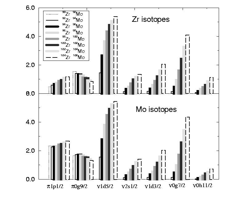
Figure 5: Orbital occupation numbers.

IV Conclusion and perspectives

We have introduced a new approach for the implementation of the Shell Model Monte Carlo method to perform shell-model calculations using non-identical proton and neutron valence spaces. General features of the SMMC method were reviewed. Differences between the isospin and the $pn$-formalisms have been pointed out; in particular, the $T_{z}$ projection has been described in detail.

The results of the SMMCpn approach have been validated in the $sd$-shell using a “good”-signed schematic interaction and in the $fp$-shell using the realistic KB3 interaction. In the latter case, we dealt with the sign problem using an extrapolation method.

As the first novel application of the SMMCpn approach, we performed a set of calculations for the even-even ${}^{90-104}\mathrm{Zr}$ and ${}^{92-106}\mathrm{Mo}$ isotopes, using a realistic effective interaction in the valence space described by ($\pi\!:$ $1p_{1/2},0g_{9/2}$) and ($\nu\!:$ $1d_{5/2},2s_{1/2},1d_{3/2},0g_{7/2},0h_{11/2}$) orbitals. A comparison of the ground-state energies of the first few nuclei in both isotope chains showed excellent agreement with the exact diagonalization results and provides a definitive test of our algorithm and the SMMCpn method. We then studied the transitional nature of the isotopes by using the $B(E2)$ strength as a gross measure of the $0_{1}^{+}-2_{1}^{+}$ separation. Along both isotope chains, we have obtained an enhancement in the $B(E2)$ strengths as a function of the added neutrons, accompanied by a quenching in the neutron-pairing correlations. In spite of this qualitative reproduction of the onset of deformations, further research clearly is needed for a qualitative result in the heavier Zr and Mo nuclei. A comparison with the experimental data suggests that this situation may be a shortcoming due to the degrees of freedom that are absent in the chosen valence space and possibly due to the value of the $0h_{11/2}$ orbital. We will investigate this further in future work.

Apart from future applications involving realistic effective interactions, use of schematic interactions in SMMCpn applications should be an interesting direction of research. Such interactions have been commonly used to calculate realistic estimates of collective properties and level densities; the latter is an important ingredient in the prediction of nuclear reaction rates in astrophysics. Parity dependence of these densities may play a crucial role in the nucleosynthesis. We believe that SMMCpn will prove to be a useful computational tool in this regard.