Precession Mode on High-$K$ Configurations: Non-Collective Axially-Symmetric Limit of Wobbling Motion

Abstract

We have studied the precession mode, the rotational excitation built on the high-$K$ isomeric state, in comparison with the recently identified wobbling mode. The random-phase-approximation (RPA) formalism, which has been developed for the nuclear wobbling motion, is invoked and the precession phonon is obtained by the non-collective axially-symmetric limit of the formalism. The excitation energies and the electromagnetic properties of the precession bands in ¹⁷⁸W are calculated, and it is found that the results of RPA calculations well correspond to those of the rotor model; the correspondence can be understood by an adiabatic approximation to the RPA phonon. As a by-product, it is also found that the problem of too small out-of-band $B(E2)$ in our previous RPA wobbling calculations can be solved by a suitable choice of the triaxial deformation which corresponds to the one used in the rotor model.

1. Introduction

In this talk, we present a recent progress of our study on the wobbling and precession modes in nuclei. These keywords, wobbling and precession, represents the motions of classical tops. They are quite interesting because they describe three-dimensional (3-D) rotational motion, and so related to a fundamental question: How does a nucleus rotate as a 3-D quantum object?

We do not know how strictly these two are distinguished, but in the following we use wobbling for motions of triaxial-body and precession for those of axially-symmetric body. In the lowest energy motion, the top rotates about one of the principal axes with largest moment of inertia, but when excited the angular momentum vector tilts from this axis in the body-fixed (intrinsic) frame. Then, looking it from the laboratory frame, the body wobbles or precesses, and that is why these names came from. In the classical mechanics, these two are similar; actually the difference is that the trajectory of the angular momentum vector is a pure circle in the case of precession, while it is an ellipse in the case of wobbling.

However, the atomic nucleus is a quantum system and the situation is dramatically changed: The collective rotation cannot occur about the symmetry axis. Thus, the quantum spectra corresponding to the wobbling and precession motions are completely different. In the case of wobbling, the spectra associated with an intrinsic configuration are composed of multiple rotational bands; the lowest (yrast) one represents the uniform rotation about the main rotation axis, the first (one-phonon) excited band represents a quantized motion of tilting angular momentum vector, and so on (more excited band with more tilting angle). These (${\mit\Delta}I=2$) rotational bands corresponds to a collective rotation about the main rotation axis with largest moment of inertia. Since the excitation of phonons, or tilting the angular momentum vector is another type of rotation about the axis perpendicular to the main rotation axis, these excitations form (${\mit\Delta}I=1$) vertical sequences. In this way, the wobbling motions show a complicated band structure, the horizontal rotational sequences and vertical phonon-like excitations.

On the other hand, the angular momentum along the symmetry axis (the main rotation axis) is generated by quasi-particle alignments in the high-$K$ isomeric configurations, and no collective rotation exists about it in the case of precession. There are no horizontal sequences leaving only one vertical band for each intrinsic configuration, which is nothing but a collective rotation about the perpendicular axis to the high-$K$ angular momentum.

Recently, the wobbling phonon spectra have been identified among the triaxial superdeformed (TSD) bands in Lu nuclei Od01 ; Jen04 , up to two-phonon excitations. By using the microscopic framework, the random-phase approximation (RPA), we have studied the wobbling phonon in the Hf-Lu region MSM02 ; MSM04 . The precession bands are rotational bands excited on the prolate high-$K$ isomers and have been known for many years, see e.g. Cul99 . We have recently investigated the properties of the precession modes applying the same RPA formalism in comparison with the wobbling modes MS05 ; SMM05 . The content of this talk is largely based on the results of SMM05 , and a further development on the out-of-band $B(E2)$ transition probability of wobbling phonon excitation (see §3).

2. Precession mode as a phonon

The study of wobbling and precession modes has a long history (see references quoted in SMM05 ). Our recent works on the wobbling motions rely on the microscopic framework developed in 1979 by Marshalek Mar79 . In almost the same time, a very important work for the precession mode have been done here in Lund in 1981 by Andersson et al. And81 (c.f. also Refs. Kura80 ; Kura82 ). In these works, was used the microscopic RPA formalism, which is known to be suitable to describe vibrational excitations. The reason why the RPA is employed for such specific rotational motions as the wobbling and precession modes can be easily understood in the case of precession band, i.e. the high-$K$ rotational band.

The spectra of high-$K$ rotor is well-known:

$$E_{{\rm high-}K}(I)=\frac{1}{2{\cal J}_{\bot}}[I(I+1)-K^{2}],\quad(I\geq K).$$ (1)

Putting $n=I-K$ and assuming $K$ is large, it is easy to see that this leads to an approximately harmonic spectrum,

$$E_{{\rm high-}K}(n)=\omega_{\rm prec}\left[n+\frac{1}{2}+\frac{n(n+1)}{K}\right],$$ (2)

where $\omega_{\rm prec}\equiv K/{\cal J}_{\bot}$ is the precession phonon energy. The remaining anharmonic term is of order $(1/K)$ and can be neglected at the high-$K$ limit. This harmonic picture is also valid for the $E2$ transitions,

$$B(E2)=(5/16\pi)\,Q_{0}^{2}\,\langle I_{f}K20|I_{i}K\rangle^{2}.$$ (3)

By taking the high-$K$ asymptotic limit in the Clebsch-Gordan coefficient,

$$\left\{\begin{array}[]{l}B(E2;n+1\rightarrow n)\propto 3[(n+1)/K],\vspace{2mm}\\ B(E2;n+2\rightarrow n)\propto(3/2)[(n+2)(n+1)/K^{2}],\end{array}\right.$$

in which the one-phonon transition is order $(1/K)$ and the direct transition to two-phonon state is $(1/K^{2})$, so that the direct two-phonon transitions are prohibited in the high-$K$ limit.

Now it is clear that the phonon picture is valid and the RPA formalism can be used to describe the precession mode microscopically, which has been done by Andersson et al. And81 . The key of their work is to adopt the so-called symmetry-restoring separable type interaction: The residual interaction used in the RPA is constructed in such a way that the rotational symmetry broken by the deformed mean-field hamiltonian is recovered. This uniquely determines the complete form of the residual interaction, and there is no adjustable parameter in the RPA calculation. The dispersion equation is simply given as $\omega\,S(\omega)=0$, where the $\omega=0$ solution is the rotational symmetry-restoring mode, i.e. the Nambu-Goldstone (NG) mode, $J_{\pm}=J_{y}\pm iJ_{z}$. Here and in the following we assume the $x$-axis as the high-$K$ alignment axis. The equation for non NG modes can be formally cast into the same form as $\omega_{\rm prec}=K/{\cal J}_{\bot}$,

$$\omega_{\rm prec}=\frac{K}{{\cal J}^{(\rm eff)}_{\bot}(\omega_{\rm prec})},$$ (4)

but with microscopically defined moment of inertia,

$${\cal J}^{(\rm eff)}_{\bot}(\omega_{\rm prec})=\frac{1}{2}\sum_{\mu<\nu}\left\{\frac{|J_{+}(\mu\nu)|^{2}}{E_{\mu\nu}-\omega_{\rm prec}}+\frac{|J_{-}(\mu\nu)|^{2}}{E_{\mu\nu}+\omega_{\rm prec}}\right\}.$$

However, the inertia ${\cal J}^{(\rm eff)}_{\bot}(\omega_{\rm prec})$ is energy-dependent and actually Eq. (4) is a non-linear equation to obtain the RPA eigen-energy. Electromagnetic transitions can be calculated as the squared amplitudes of the RPA phonon $X^{\dagger}_{\rm prec}$ with respect to appropriate transition operators $Q_{\lambda\mu}$:

$$B(\lambda)_{{\mit\Delta}I}\approx\left|\langle K|[Q_{\lambda\mu={\mit\Delta}I},X^{\dagger}_{\rm prec}]|K\rangle\right|^{2}\,\,(K\gg 1).$$ (5)

Here it should be stressed that this RPA formalism of Andersson et al. is obtained by taking the non-collective axially symmetric limit ($\gamma=60^{\circ}$ or $-120^{\circ}$ in the Lund convention) of the RPA wobbling formalism of Marshalek SMM05 . In this way, the precession and wobbling can be considered as similar kinds of collective excitation modes.

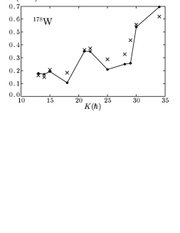
Figure 1: Excitation energies of the one-phonon precession modes excited on high-$K$ configurations. Calculated ones are denoted by filled circles connected by solid lines, and experimental ones by crosses. Taken from Ref. SMM05 .

The results of RPA calculations for precession modes in ¹⁷⁸W Cul99 are presented in Fig. 1. In this nucleus there observed many high-$K$ isomers, on which the rotational bands exist: Eleven isomers investigated are ranging from four-quasiparticle states ($2\nu$-$2\pi$) to ten-quasiparticle states ($6\nu$-$4\pi$). We have used the Nilsson potential as a mean field with appropriate deformation parameters and pairing gap parameters. Except for four cases, $K^{\pi}=18^{-},\,25^{+},\,28^{-},\,29^{+}$, the one-phonon excitation energies are well reproduced. As for these four isomers, the precession energies are too small; namely, the calculated moments of inertia are too large. We found that the overestimation of the calculated moments of inertia is due to the proton contributions in these four configurations, which include the $\pi[541]1/2^{-}$ Nilsson state originated from the $\pi h_{9/2}$ high-$j$ decoupled orbit. Apparently the contribution from this orbit is overestimated in the present calculations, see Ref. SMM05 for more detailed discussions.

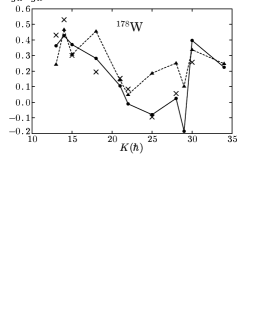
Figure 2: $(g_{K}-g_{R})$-factors for high-$K$ precession bands. Those calculated by the RPA are denoted by filled circles connected by solid lines, while those by the mean-field approximation by filled triangles connected by dotted lines. Those extracted from the experimental data are shown by crosses. Taken from Ref. SMM05 .

As for the electromagnetic transitions, one can directly compare the calculated and measured transition probabilities, but here we compare them in a different way. As is well-known, the rotor model gives simple formula for transition probabilities, e.g. Eq. (3) for $B(E2)$. Thus, by using the asymptotic forms of the Clebsch-Gordan coefficients, $B(E2)$ and $B(M1)$ are parameterized in the high-$K$ limit as,

$$B(E2:K+1\rightarrow K)_{\rm rot} \approx \frac{15}{16\pi}\frac{1}{K}Q_{0}^{2},$$ (6)

$$B(M1:K+1\rightarrow K)_{\rm rot} \approx \frac{3}{4\pi}\left(g_{K}-g_{R}\right)^{2}K.$$ (7)

On the other hand, they are calculated by Eq. (5) in the RPA formalism. By equating these two expressions, we define $Q$ moment or $g_{K}-g_{R}$ factor calculated within the RPA. Namely, we parameterize the results of RPA calculations in the same way as the rotor model, and they are compared with experimentally extracted ones in Fig. 2 for $B(M1)$. In this figure we included the results of the simple mean-field approximation, namely using $g_{K}$ calculated as $\langle\mu_{x}\rangle/\langle J_{x}\rangle$ ($\mu_{x}$ is the $M1$ operator) with each high-$K$ state, and a common value of $g_{R}$ calculated in the same way but with the ground state. As it is clearly seen in Fig. 2, the RPA calculation gives a much better description of $B(M1)$ values. As for the $E2$ transitions, there is no experimental data available, but by comparing the calculated RPA $Q$ moments with the mean-field estimate of $Q$ moments it is found that they well coincide except four configurations, which include the $\pi h_{9/2}$ decoupled orbit (the figure is not shown, see Ref. SMM05 ).

The results for the excitation energies and transition probabilities indicate that the high-$K$ rotor model picture is realized if the model parameters, moment of inertia, $Q$ moment and $g$-factors, are calculated appropriately by means of the RPA. This fact can be naturally understood by using an adiabatic approximation studied in Refs. Kura80 ; Kura82 ; i.e. in this approximation, $X_{\rm prec}^{\dagger}\approx(J_{+}+K\,i{\mit\Theta}_{+})_{\rm RPA}/\sqrt{2K}$, while the NG mode is $X_{\rm NG}^{\dagger}=J_{-}/\sqrt{2K}$. By using this form it is easy to confirm, for example, $(Q_{0})_{\rm mean-field}\approx(Q_{0})_{\rm RPA}$; the situation is more complicated for the $g$-factors, see Ref. SMM05 for more detailed discussions.

3. Out-of-band transition of wobbling phonon

Now let us come back to the case of wobbling mode. It has been shown that the RPA calculation well corresponds to the rotor model picture in the case of precession, especially for $B(E2)$. It can be shown that a similar consideration in term of the adiabatic approximation can be also applied for the wobbling mode. However, the $B(E2)$ value of our RPA wobbling calculations in Lu nuclei were too small, by about 1/2 $-$ 1/3, compared with the experimental data, whose magnitudes are well reproduced by the rotor model. This has been a serious problem for us, see Fig. 3 and Refs.MSM02 ; MSM04 . Considering the results of the precession modes, however, it is difficult to understand the discrepancy between results of the RPA calculation and the rotor model. Therefore, we looked for the reason why the RPA calculation gave such smaller values.

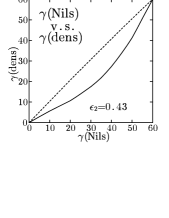
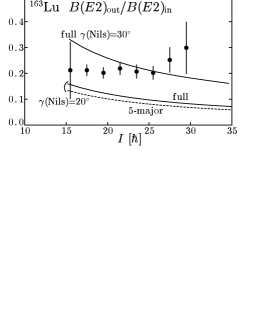
Figure 3: Upper panel: The relation between $\gamma({\rm Nils})$ and $\gamma({\rm dens})$ for the TSD band in ¹⁶³Lu. Lower panel: Comparison of the out-of-band to in-band $B(E2)$ ratios; symbols are the experimental data, three curves are corresponding results of RPA calculations, in which the dashed line is the result of Ref. MSM02 , see text for detail.

We have found that there are two reasons: One is related to the model space of the RPA calculations, and the other is to the definition of triaxiality parameter $\gamma$ in the Nilsson potential. As for the model space, we used the 5-major shells but it was not enough; this effect, however, is only about 20% and not the major effect. More important is the value of the $\gamma$ parameter. It is believed that the $\gamma$ value is about $20^{\circ}$ in the TSD bands in the Lu region. We have used $20^{\circ}$ for the $\gamma$ in the Nilsson potential, $\gamma({\rm Nils})=20^{\circ}$. It is found, however, that the $\gamma$-value defined by the density distribution, $\gamma({\rm dens)}$, is only about $10^{\circ}$. Here, $\gamma({\rm dens)}$ is defined by the expectation values of the quadrupole operators (the Lund convention for sign of $\gamma$), $-\tan^{-1}\langle Q_{22}^{(+)}\rangle/\langle Q_{20}^{(+)}\rangle$, i.e.

$$\gamma({\rm dens})=\tan^{-1}\frac{\sqrt{3}\,\displaystyle\langle\sum_{a=1}^{A}(y^{2}-x^{2})_{a}\rangle}{\displaystyle\langle\sum_{a=1}^{A}(2z^{2}-x^{2}-y^{2})_{a}\rangle}.$$ (8)

Of course, the triaxiality of the rotor model should be that of the density distribution. By using an assumption for moments of inertia, ${\cal J}_{y}={\cal J}_{z}$, in the triaxial rotor model, the out-of-band to in-band $B(E2)$ ratio depends on the $\gamma$ parameter like $B(E2)_{\rm out}/B(E2)_{\rm in}\propto\tan^{2}{(\gamma+30^{\circ})}$ Ham03 . Even in general cases with ${\cal J}_{y}\neq{\cal J}_{z}$, this $\gamma$-dependence approximately follows. Then it is easy to see that the difference of this ratio at $\gamma=10^{\circ}$ and $20^{\circ}$ is about factor two. The $\gamma$ value corresponding to $\gamma({\rm dens)}=20^{\circ}$ in the density distribution is about $\gamma({\rm Nils)}\approx 30^{\circ}$ in the Nilsson potential (see Fig. 3). The results of the RPA calculation using different $\gamma$-values are shown in Fig. 3, where the relation between $\gamma({\rm dens)}$ and $\gamma({\rm Nils)}$ is also depicted in the upper panel. The dashed line with the model space of the 5-major shells is the result of Ref. MSM02 . As is shown in the figure, if one uses the full model space and $\gamma({\rm Nils)}=30^{\circ}$, the $B(E2)$ ratio comes up to the correct magnitude just like in the case of the rotor model Gor04 .

The discrepancy between $\gamma({\rm Nils)}$ and $\gamma({\rm dens)}$ is just a matter of definition, see e.g. Appendix of Ref. SM84 . For the pure harmonic oscillator potential, the definition of $\gamma({\rm Nils)}$ gives

$$\gamma({\rm Nils})=\tan^{-1}\frac{\sqrt{3}\,(\omega_{y}-\omega_{x})}{2\omega_{z}-\omega_{x}-\omega_{y}}.$$ (9)

The selfconsistency of the potential (Mottelson condition), $\langle\sum_{a=1}^{A}(x_{k}^{2})_{a}\rangle\propto 1/\omega_{k}^{2}$ ($k=x,y,z$), is approximately satisfied in the Nilsson potential, and then by Eq. (8),

$$\gamma({\rm dens})\approx\gamma({\rm self})=\tan^{-1}\frac{\sqrt{3}\,(1/\omega^{2}_{y}-1/\omega^{2}_{x})}{2/\omega^{2}_{z}-1/\omega^{2}_{x}-1/\omega^{2}_{y}},$$ (10)

where $\gamma({\rm self})$ is the triaxiality based on the shape (ellipsoid) of an equi-potential surface for the anisotropic harmonic oscillator. In this way the relation between $\gamma({\rm Nils)}$ and $\gamma({\rm dens)}$ in the upper panel of Fig. 3 can be naturally understood.

4. Summary

The RPA precession formalism by Andersson et al. can be obtained by a non-collective axially-symmetric limit of the RPA wobbling formalism by Marshalek. By using this formalism, it is shown that the RPA calculation gives fairly good agreements for both the excitation energies and $B(M1)$ transitions for the precession phonons on high-$K$ isomers in ¹⁷⁸W. This result can be interpreted by an adiabatic approximation, and shows a good correspondence between the RPA calculation and the rotor model; especially $B(E2)$ or $Q$ moments, and $B(M1)$ or $g$-factors SMM05 .

There is an important feed back to the calculation of recently observed nuclear wobbling motions. The problem of small $B(E2)$ ratios in our previous RPA calculations can be solved if one uses a proper value of the triaxiality parameter $\gamma({\rm dens})\approx 20^{\circ}$ in the density distribution. This does not completely solve the problem, however, because the Nilsson-Strutinsky calculation gives minima at $\gamma({\rm Nils})\approx 20^{\circ}$ in the Nilsson potential, which corresponds to $\gamma({\rm dens})\approx 10^{\circ}$. Thus, it raises a more fundamental question; why the Nilsson-Strutinsky calculation does not provide enough triaxiality, which is required for explaining the measured $B(E2)$ ratio of the wobbling phonon band. Finally, it is shown that the RPA can describe the 3-D rotational motion (in the small amplitude approximation) at least as the same level as the rotor model. In other words, the rotor model may be justified by the microscopic RPA calculations.

Acknowledgments

This work was supported by the Grant-in-Aid for Scientific Research (No. 16540249) from the Japan Society for the Promotion of Science.

References

- (1) S. W. Ødegård et al., Phys. Rev. Lett. 86, 5866 (2001).
- (2) D. R. Jensen et al., Eur. Phys. J. A 19, 173 (2004).
- (3) M. Matsuzaki, Y. R. Shimizu and K. Matsuyanagi, Phys. Rev. C 65, 041303(R) (2002).
- (4) M. Matsuzaki, Y. R. Shimizu and K. Matsuyanagi, Phys. Rev. C 69, 034325 (2004).
- (5) M. Matsuzaki and Y. R. Shimizu, nucl-th/0412009, Prog. Theor. Phys. 114, in press (2005).
- (6) Y. R. Shimizu, M. Matsuzaki and K. Matsuyanagi, Phys. Rev. C 72, 014306 (2005).
- (7) D. M. Cullen et al., Phys. Rev. C 60, 064301 (1999).
- (8) E. R. Marshalek, Nucl. Phys. A 331, 429 (1979).
- (9) C. G. Andersson, J. Krumlinde, G. Leander and Z. Szymański, Nucl. Phys. A 361, 147 (1981).
- (10) H. Kurasawa, Prog. Theor. Phys. 64, 2055 (1980).
- (11) H. Kurasawa, Prog. Theor. Phys. 68, 1594 (1982).
- (12) I. Hamamoto and G. B. Hagemann, Phys. Rev. C 67, 014319 (2003).
- (13) A. Görgen et al., Phys. Rev. C 69, 031301 (2004).
- (14) Y. R. Shimizu and K. Matsuyanagi, Prog. Theor. Phys. 71, 799 (1984).