Analyzing $\eta^{\prime}$ photoproduction data on the proton at energies of 1.5–2.3 GeV

Abstract

The recent high-precision data for the reaction $\gamma p\to p\eta^{\prime}$ at photon energies in the range 1.5–2.3 GeV obtained by the CLAS collaboration at the Jefferson Laboratory have been analyzed within an extended version of the photoproduction model developed previously by the authors based on a relativistic meson-exchange model of hadronic interactions [Phys. Rev. C 69, 065212 (2004)]. The $\eta^{\prime}$ photoproduction can be described quite well over the entire energy range of available data by considering $S_{11}$, $P_{11}$, $P_{13}$, and $D_{13}$ resonances, in addition to the $t$-channel mesonic currents. The observed angular distribution is due to the interference between the $t$-channel and the nucleon $s$- and $u$-channel resonance contributions. The $j=3/2$ resonances are required to reproduce some of the details of the measured angular distribution. For the resonances considered, our analysis yields mass values compatible with those advocated by the Particle Data Group. We emphasize, however, that cross-section data alone are unable to pin down the resonance parameters and it is shown that the beam and/or target asymmetries impose more stringent constraints on these parameter values. It is found that the nucleonic current is relatively small and that the $NN\eta^{\prime}$ coupling constant is not expected to be much larger than 2.

I Introduction

One of the primary interests in investigating the $\eta^{\prime}$ photoproduction reaction is that it may be suited to extract information on nucleon resonances, $N^{*}$, in the less explored higher $N^{*}$ mass region. Current knowledge of most of the nucleon resonances is mainly due to the study of $\pi N$ scattering and/or pion photoproduction off the nucleon. Since the $\eta^{\prime}$ meson is much heavier than a pion, $\eta^{\prime}$ meson-production processes near threshold necessarily sample a much higher resonance-mass region than the corresponding pion production processes. They are well-suited, therefore, for investigating high-mass resonances in low partial-wave states. Furthermore, reaction processes such as $\eta^{\prime}$ photoproduction provide opportunities to study those resonances that couple only weakly to pions, in particular, those referred to as “missing resonances”, which are predicted by quark models, but not found in more traditional pion-production reactions Capstick1 .

Another special interest in $\eta^{\prime}$ photoproduction is the possibility to impose a more stringent constraint on its yet poorly known coupling strength to the nucleon. This has attracted much attention in connection with the so-called “nucleon-spin crisis” in polarized deep inelastic lepton scattering EMC88 . In the zero-squared-momentum limit, the $NN\eta^{\prime}$ coupling constant $g_{NN\eta^{\prime}}(q^{2}=0)$ is related to the flavor-singlet axial charge $G_{A}$ through the flavor singlet Goldberger–Treiman relation Shore (see also Refs. Efremov ; Venez1 ; Feldmann )

$$2m_{N}\,G_{A}(0)=F\,g_{NN\eta^{\prime}}(0)+{\frac{F^{2}}{2N_{F}}}\,m_{\eta^{\prime}}^{2}\,g_{NNG}(0)~{},$$ (1)

where $F$ is a renormalization-group invariant decay constant defined in Ref. Shore , $N_{F}$ is the number of flavors, and $m_{N}$ and $m_{\eta^{\prime}}$ are the nucleon and $\eta^{\prime}$ masses, respectively; $g_{NNG}$ describes the coupling of the nucleon to the gluons arising from contributions violating the Okubo-Zweig-Iizuka (OZI) rule OZI . The EMC collaboration EMC88 has measured an unexpectedly small value of $G_{A}(0)\approx 0.20\pm 0.35$; a more recent analysis of the SMC collaboration SMC97 yields a comparable value of $G_{A}(0)\approx 0.16\pm 0.10$. The first term on the right-hand side of the above equation corresponds to the quark contribution to the “spin” of the proton, and the second term to the gluon contribution Venez1 ; x1 . Therefore, once $g_{NN\eta^{\prime}}(0)$ is known, Eq. (1) may be used to extract the coupling $g_{NNG}(0)$. Unfortunately, however, there is no direct experimental measurement of $g_{NN\eta^{\prime}}(0)$ so far. Reaction processes where the $\eta^{\prime}$ meson is produced directly off a nucleon may thus offer a unique opportunity to extract this coupling constant. Here it should be emphasized that, as has been pointed out in Ref. NH1 , hadronic model calculations such as the present one cannot determine the $NN\eta^{\prime}$ coupling constant in a model-independent way. At best, we get an estimate for the range of its value at the on-shell kinematic point, i.e., at $q^{2}=m_{\eta^{\prime}}^{2}$. Assuming the usual behavior of hadronic form factors for off-shell mesons which generally decrease for $q^{2}<m^{2}$, we expect then that an eventually small upper limit of $g_{NN\eta^{\prime}}(q^{2}=m_{\eta^{\prime}}^{2})$ would lead to an even smaller value of $g_{NN\eta^{\prime}}(0)$, which is needed in Eq. (1) to extract $g_{NNG}(0)$.

The major purpose of the present work is to perform an analysis of the $\gamma p\rightarrow p\eta^{\prime}$ reaction within an extended version of the relativistic meson-exchange model of hadronic interactions as reported in Ref. NH1 . This analysis is motivated by the new high-precision cross-section data obtained by the CLAS collaboration CLAS at the Jefferson Laboratory (JLab). The new data supersede the previous SAPHIR data SAPHIR analyzed in Ref. NH1 both in absolute normalization and angular shape. Also, the new CLAS data are much more accurate and, as such, may reveal features that were not seen in the analysis of the SAPHIR data.

The present paper is organized as follows. In Sec. II the extension of our model NH1 for $\gamma p\rightarrow p\eta^{\prime}$ is given. The results of the corresponding model calculations are presented in Sec. III. Section IV contains a summary with our conclusions. Some technical details of the present model are given in the Appendix.

II Formalism

The dynamical content of the present $\eta^{\prime}$ photoproduction calculation is summarized by the graphs of Fig. 1 where we employ form factors at the vertices to account for the hadronic structure. The gauge invariance of this production current is ensured by a phenomenological contact current, according to the prescription of Refs. hh97g ; hhtree98 ; dw2 . This contact term provides a rough phenomenological description of the final-state interaction which is not treated explicitly here. The basic details of the present approach are the same as in our previous paper NH1 and we will not repeat them here. There are, however, a few improvements and those will be discussed here.

II.1 Spin-3/2 resonances

The present fits also require the inclusion of spin-3/2 resonances, denoted generically by $N^{*}$. The Lagrangian for the hadronic $NN^{*}\eta^{\prime}$ interaction is given by

$$\mathcal{L}^{(\pm)}_{NN^{*}\eta^{\prime}}=\frac{g_{NN^{*}\eta^{\prime}}}{m_{\eta^{\prime}}}{\bar{N}^{*\mu}}\Theta_{\mu\nu}(z)\Gamma^{(\pm)}N\partial^{\nu}\,\eta^{\prime}+\text{H.\,c.}~{},$$ (2)

where $N^{*\mu}$, $N$, and $\eta^{\prime}$ are the resonance, nucleon, and meson fields, respectively, and

$$\Gamma^{(+)}=\gamma_{5}\quad\text{and}\quad\Gamma^{(-)}=1$$ (3)

pertain to positive- and negative-parity resonances, respectively. For the coupling tensor, $\Theta_{\mu\nu}=g_{\mu\nu}-(z+\frac{1}{2})\gamma_{\mu}\gamma_{\nu}$, we take $z=-\frac{1}{2}$ for the off-shell parameter for simplicity. The Lagrangian for the electromagnetic transition current reads

$$\mathcal{L}^{(\pm)}_{NN^{*}\gamma} =-ie\frac{g_{1NN^{*}\gamma}}{m_{N^{*}}}{\bar{N}^{*\beta}}\Theta_{\beta\mu}\Gamma^{(\pm)}\gamma_{\nu}NF^{\mu\nu}$$

$$\quad\mbox{}-e\frac{g_{2NN^{*}\gamma}}{2m^{2}_{N^{*}}}\left(\partial_{\nu}\bar{N}^{*\beta}\Theta_{\beta\mu}\Gamma^{(\pm)}N\right)F^{\mu\nu}+\text{H.\,c.}~{},$$ (4)

where $F^{\mu\nu}=\partial^{\mu}A^{\nu}-\partial^{\nu}A^{\mu}$ is the electromagnetic field-strength tensor (with $A^{\mu}$ being the vector potential).

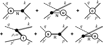
Figure 1: Diagrams contributing to $\gamma p\to\eta^{\prime}p$. Time proceeds from right to left. The intermediate baryon states are denoted N for the nucleon, and R for the $S_{11}$, $P_{11}$, $P_{13}$, and $D_{13}$ resonances. The intermediate mesons in the $t$-channel are $\rho$ and $\omega$. The external legs are labeled by the four-momenta of the respective particles and the labels s, u, and t of the hadronic vertices correspond to the off-shell Mandelstam variables of the respective intermediate particles. The three diagrams in the lower part of the diagram are transverse individually; the three diagrams in the upper part are made gauge-invariant by an appropriate choice for the contact current depicted in the top-right diagram. The nucleonic current (nuc) referred to in the text corresponds to the top line of diagrams; the meson-exchange current (mec) and resonance current contributions correspond, respectively, to the leftmost diagram and the two diagrams on the right of the bottom line of diagrams.

II.2 Energy-dependent resonance widths

For the present application, we have adapted our formalism to accommodate energy-dependent resonance widths with the appropriate threshold behavior.

For a spin-1/2 resonance propagator, we use the ansatz

$$S_{1/2}(p)=\frac{1}{{p\!\!\!/}-m_{R}+\frac{i}{2}\Gamma}=\frac{{p\!\!\!/}+m_{R}}{p^{2}-m_{R}^{2}+\frac{i}{2}({p\!\!\!/}+m_{R})\Gamma}~{},$$ (5)

where $m_{R}$ is the mass of the resonance with four-momentum $p$. $\Gamma$ is the width function whose functional behavior will be given below.

For spin-3/2, the resonant propagator reads in a schematic matrix notation

$$S_{3/2}(p)=\left[({p\!\!\!/}-m_{R})g-i\frac{\Delta}{2}\Gamma\right]^{-1}\Delta~{}.$$ (6)

All indices are suppressed here, i.e., $g$ is the metric tensor and $\Delta$ is the Rarita–Schwinger tensor written in full detail as

$$\Delta^{\mu\nu}_{\beta\alpha}=-g^{\mu\nu}\delta_{\beta\alpha}+\frac{1}{3}\gamma^{\mu}_{\beta\varepsilon}\gamma^{\nu}_{\varepsilon\alpha}+\frac{2p^{\mu}p^{\nu}}{3m_{R}^{2}}\delta_{\beta\alpha}+\frac{\gamma^{\mu}_{\beta\alpha}p^{\nu}-p^{\mu}\gamma^{\nu}_{\beta\alpha}}{3m_{R}}~{},$$ (7)

where $\beta$, $\alpha$, and $\varepsilon$ enumerate the four indices of the $\gamma$-matrix components (summation over $\varepsilon$ is implied). The inversion in (6) is to be understood on the full 16-dimensional space of the four Lorentz indices and the four components of the gamma matrices. The motivation for the ansatz (6) and the technical details how to perform this inversion is given in the Appendix.

In both cases, we write the width $\Gamma$ as a function of $W=\sqrt{s}$ according to

$$\Gamma(W)=\Gamma_{R}\left[\sum_{i=1}^{N}\beta_{i}\hat{\Gamma}_{i}(W)+\sum_{j=1}^{N_{\gamma}}\gamma_{j}\hat{\Gamma}_{\gamma_{j}}(W)\right]~{},$$ (8)

where the sums over $i$ and $j$ respectively account for decays of the resonance into $N$ two- or three-hadron channels and into $N_{\gamma}$ radiative decay channels. The total static resonance width is denoted by $\Gamma_{R}$ and the numerical factors $\beta_{i}$ and $\gamma_{j}$ (with $0\leq\beta_{i},\gamma_{j}\leq 1$) describe the branching ratios into the various decay channels, i.e.,

$$\sum_{i=1}^{N}\beta_{i}+\sum_{j=1}^{N_{\gamma}}\gamma_{j}=1~{}.$$ (9)

Similar to Refs. walker ; arndt90 ; lvov97 ; drechsel , we parameterize the width functions $\hat{\Gamma}_{i}$ and $\hat{\Gamma}_{\gamma_{j}}$ (which are both normalized to unity at $W=m_{R}$) to provide the correct respective threshold behaviors.

For the decay of the resonance into two hadronic fragments with masses ${m_{i}}_{1}$ and ${m_{i}}_{2}$, the hadronic width functions $\hat{\Gamma}_{i}$ are taken as

$$\hat{\Gamma}_{i}(W)=\left(\frac{\mathrm{q}_{i}}{\mathrm{q}_{iR}}\right)^{2L+1}\left(\frac{\lambda_{i}^{2}+\mathrm{q}^{2}_{iR}}{\lambda_{i}^{2}+\mathrm{q}^{2}_{i}}\right)^{L}D_{i}(W)$$ (10)

for $W>{m_{i}}_{1}+{m_{i}}_{2}$, and zero otherwise. $L$ denotes the partial wave in which the resonance is found and the momentum $\mathrm{q}_{i}$ is the magnitude of the center-of-momentum three-momentum of the two fragments, i.e.,

$$\mathrm{q}_{i}(W)=\frac{\sqrt{\left[W^{2}-({m_{i}}_{1}+{m_{i}}_{2})^{2}\right]\left[W^{2}-({m_{i}}_{1}-{m_{i}}_{2})^{2}\right]}}{2W}$$ (11)

and $\mathrm{q}_{iR}=\mathrm{q}_{i}(m_{R})$. For the decay of the resonance into one baryon and two mesons (for example, $N\pi\pi$), we use

$$\hat{\Gamma}_{i}(W)=\left(\frac{\mathrm{q}_{i}}{\mathrm{q}_{iR}}\right)^{2L+4}\left(\frac{\lambda_{i}^{2}+\mathrm{q}^{2}_{iR}}{\lambda_{i}^{2}+\mathrm{q}^{2}_{i}}\right)^{L+2}D_{i}(W)~{},$$ (12)

where ${m_{i}}_{2}$ in (11) needs to be replaced by the sum of the two meson masses for this case, and ${m_{i}}_{1}$ is the baryon mass. In principle, the factor

$$D_{i}(W)=\left(\frac{m_{R}}{W}\right)^{n_{i}}~{},\quad\text{with}\quad n_{i}\geq 0~{},$$ (13)

allows for a modification of the asymptotic behavior of $\hat{\Gamma}_{i}(W)$, however, we use $n_{i}=0$ throughout for simplicity. The parameter $\lambda_{i}$ is an inverse range parameter; since we found very little sensitivity to varying this parameter (within reasonable ranges), we kept it fixed at $\lambda_{i}=1\,\text{fm}^{-1}$ for all channels.

The width function $\hat{\Gamma}_{\gamma_{j}}$ for the decay into a hadron with mass $m_{j}$ and a photon with three-momentum $\mathrm{k}_{j}$ is taken as

$$\hat{\Gamma}_{\gamma_{j}}(W)=\left(\frac{\mathrm{k}_{j}}{\mathrm{k}_{jR}}\right)^{2L+2}\left(\frac{\lambda_{\gamma_{j}}^{2}+\mathrm{k}^{2}_{jR}}{\lambda_{\gamma_{j}}^{2}+\mathrm{k}^{2}_{j}}\right)^{L+1}D_{\gamma_{j}}(W)~{},$$ (14)

where

$$\mathrm{k}_{j}(W)=\frac{W^{2}-m_{j}^{2}}{2W}$$ (15)

for $W>m_{j}$, and zero otherwise, and $\mathrm{k}_{jR}=\mathrm{k}_{j}(m_{R})$. As in the hadronic case, the asymptotic damping function is given by

$$D_{\gamma_{j}}(W)=\left(\frac{m_{R}}{W}\right)^{r_{j}}~{},\quad\text{with}\quad r_{j}\geq 0~{}.$$ (16)

Again, for simplicity, we employ $r_{j}=0$ throughout. In practice, for the present case, the photon decay channels are negligibly small and play no role for the total width. The corresponding branching ratio $\gamma_{N\gamma}$ for the $N\gamma$ channel is only needed to extract the value of the $N\eta^{\prime}$ branching ratio $\beta_{N\eta^{\prime}}$ (see below).

III Results and Discussion

Before we discuss the details of our results, some general remarks are in order. The basic strategy of our model approach is to start with the nucleon plus meson-exchange currents and add the resonances one by one as needed in the fitting procedure until one achieves a reasonable fit of the new $\eta^{\prime}$ photoproduction data obtained by the CLAS collaboration CLAS . We allow for both spin-1/2 and -3/2 resonances in our model. Our quantitative criterion for a reasonable fit was to discard all fits with a $\chi^{2}$ per data point of $\chi^{2}/N>1.3$, which is supported by the fact that fits with $\chi^{2}/N$ much larger than 1.3 are noticeably of inferior fit quality even for the naked eye. Under this criterion, we found that one needs at least four resonances in order to obtain a reasonable fit in the present approach. We find, in particular, that, in addition to spin-1/2 resonances, spin-3/2 resonances are necessary to achieve acceptable fits. In this respect, we emphasize that the SAPHIR data SAPHIR analyzed in Ref. NH1 have rather large error bars. While not entirely incompatible with the new high-precision CLAS data CLAS , they clearly are less constraining than the CLAS data, which may explain why there was no need for spin-3/2 resonances in our previous work.

As we have pointed out in Ref. NH1 , the cross-section data alone are unable to pin down the model parameters and, therefore, one finds different sets of parameters which fit the data equally well. Note that this is not due to the uncertainties in the data, but simply because, intrinsically, the cross sections do not impose enough stringent constraints on the fit. In particular, for each resonance, the resulting fitted mass value depends to a certain extent on its starting value in the fitting procedure. The starting (resonance) mass values we consider here generally are around those advocated by the Particle Data Group (PDG) PDG .

In the present work, in the case of those resonances that can be identified with known PDG resonances, we have taken into account only the corresponding dominant branching ratios $\beta_{i}$ from the PDG for hadronic decays when this information is available (and we ignored the fact that some of the quoted branching ratios are subject to large uncertainties). If no information is available, we consider only the $N\pi$ partial decay, with the corresponding branching ratio $\beta_{N\pi}$ as a free fit parameter. Apart from these branching ratios, we also consider the $N\eta^{\prime}$ branching ratio $\beta_{N\eta^{\prime}}$ which is calculated from the product of the coupling constants $g_{NN^{*}\eta^{\prime}}g_{NN^{*}\gamma}$ in conjunction with the assumed branching ratio $\gamma_{N\gamma}$ for the radiative decay. In the following tables, therefore, $\beta_{N\eta^{\prime}}$ is not an independent fit parameter, but rather a parameter extracted from the fitted values of the product $g_{NN^{*}\eta^{\prime}}g_{NN^{*}\gamma}$.

One might expect that the way in which the energy dependence is implemented in the resonance width in the present work [cf. Eqs. (12)–(14)] may introduce a considerable uncertainty in the final results. However, we find that the cross sections are not very sensitive to our assumptions in this respect. In fact, we also re-ran some of the cross-section fits discussed below using step functions for the widths that switch on the full partial widths at the corresponding thresholds without any smooth energy dependence and we found that the parameter sets obtained in this way were fairly close to the ones reported here. For spin observables, however, this insensitivity does not hold true. In particular, the beam and target asymmetries are rather sensitive to how the energy dependence of the width is treated and one must be careful then when confronting model predictions with the data when the latter should become available.

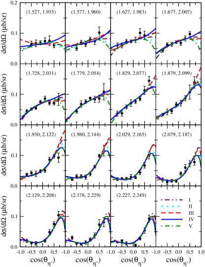
Figure 2: (Color online) Differential cross section for $\gamma p\to p\eta^{\prime}$ according to the mechanisms shown in Fig. 1 as a function of the $\eta^{\prime}$ emission angle $\theta_{\eta^{\prime}}$ in the center-of-momentum frame of the system. As indicated in the legend, the curves correspond to the fit results of Tables 1 (dash-double-dotted), 2 (dotted lines), 3 (dashed), 4 (solid), and 5 (dash-dotted). The numbers ($T\gamma,W$) in parentheses are the incident photon energy $T_{\gamma}$ and the corresponding $s$-channel energy $W=\sqrt{s}$, respectively, in GeV. The data are from Ref. CLAS .

We now turn to the discussion of the details of our analysis. We emphasize that the results shown here do not necessarily have the lowest $\chi^{2}$. Rather, they are sample fit results that illustrate the different dynamical features one may obtain considering only the currently available data in the analysis within the fit-quality criteria mentioned above.

Table 1: Model parameters fitted to the $\gamma p\to\eta^{\prime}p$. (See text, and also Ref. NH1 , for explanations of parameters.) Values in boldface are not fitted. The branching ratios $\gamma_{N\gamma}$ are assumptions made to extract $\beta_{N\eta^{\prime}}$ (for the total width, however, the $\gamma_{N\gamma}$ values are too small to be relevant). The starting values for fitting all resonance masses were chosen here within the energy range covered by the data set. $\chi^{2}/N=1.19$.

Nucleonic current:
$g_{NN\eta^{\prime}}$	0.43
$\lambda$	0.0
$\Lambda_{N}$ (MeV)	1200
Mesonic current:
$g_{\eta^{\prime}\rho\gamma}$	1.25
$g_{\eta^{\prime}\omega\gamma}$	0.44
$\Lambda_{v}$ (MeV)	1275
$N^{*}=S_{11}$ current:
$m_{N^{*}}$ (MeV)	1958
$g_{NN^{*}\gamma}\,g_{NN^{*}\eta^{\prime}}$	0.25
$\lambda$	1.00
$\Lambda_{N^{*}}$ (MeV)	1200
$\Gamma_{N^{*}}$ (MeV)	139
$\gamma_{N\gamma}$	0.002
$\beta_{N\pi}$	0.50
$\beta_{N\eta^{\prime}}$	0.50
$N^{*}=P_{11}$ current:
$m_{N^{*}}$ (MeV)	2104
$g_{NN^{*}\gamma}\,g_{NN^{*}\eta^{\prime}}$	0.80
$\lambda$	1.00
$\Lambda_{N^{*}}$ (MeV)	1200
$\Gamma_{N^{*}}$ (MeV)	136
$\gamma_{N\gamma}$	0.002
$\beta_{N\pi}$	0.36
$\beta_{N\eta^{\prime}}$	0.64
$N^{*}=P_{13}$ current:
$m_{N^{*}}$ (MeV)	1885
$g_{1NN^{*}\gamma}\,g_{NN^{*}\eta^{\prime}}$	0.01
$g_{2NN^{*}\gamma}\,g_{NN^{*}\eta^{\prime}}$	0.17
$\Lambda_{N^{*}}$ (MeV)	1200
$\Gamma_{N^{*}}$ (MeV)	59
$\beta_{N\pi}$	0.6
$\beta_{N\omega}$	0.4
$N^{*}=D_{13}$ current:
$m_{N^{*}}$ (MeV)	1823
$g_{1NN^{*}\gamma}\,g_{NN^{*}\eta^{\prime}}$	0.47
$g_{2NN^{*}\gamma}\,g_{NN^{*}\eta^{\prime}}$	-0.65
$\Gamma_{N^{*}}$ (MeV)	450
$\gamma_{N\gamma}$	0.002
$\beta_{N\pi}$	1.00

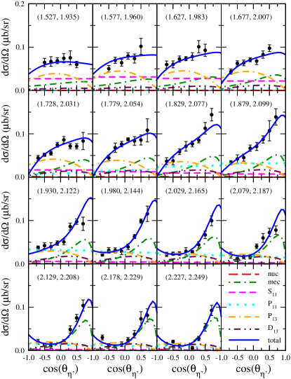
Figure 3: (Color online) Differential cross sections and the dynamical content of the present model corresponding to the fit result of Table 1. The dash-dotted curves correspond to the mesonic current contribution; the dashed curves to the $S_{11}$ resonance current and the dotted curves to the $P_{11}$ resonance. The dot–double-dashed curves correspond to the $P_{13}$ resonance current while the dash–double-dotted curves show the $D_{13}$ resonance contribution. The solid curves correspond to the total current. The nucleonic current contribution (long-dashed curves) is very small and cannot be seen on the present scale.

Table 2: Same as Table. 1. An additional $D_{13}$ resonance was included here to see whether this would improve the fit quality. $\chi^{2}/N=1.04$.

Nucleonic current:
$g_{NN\eta^{\prime}}$	0.25
$\lambda$	0.0
$\Lambda_{N}$ (MeV)	1200
Mesonic current:
$g_{\eta^{\prime}\rho\gamma}$	1.25
$g_{\eta^{\prime}\omega\gamma}$	0.44
$\Lambda_{v}$ (MeV)	1308
$N^{*}=S_{11}$ current:
$m_{N^{*}}$ (MeV)	1925
$g_{NN^{*}\gamma}\,g_{NN^{*}\eta^{\prime}}$	0.08
$\lambda$	0.58
$\Lambda_{N^{*}}$ (MeV)	1200
$\Gamma_{N^{*}}$ (MeV)	40
$\gamma_{N\gamma}$	0.002
$\beta_{N\pi}$	0.56
$\beta_{N\eta^{\prime}}$	0.44
$N^{*}=P_{11}$ current:
$m_{N^{*}}$ (MeV)	1991
$g_{NN^{*}\gamma}\,g_{NN^{*}\eta^{\prime}}$	-1.69
$\lambda$	0.09
$\Lambda_{N^{*}}$ (MeV)	1200
$\Gamma_{N^{*}}$ (MeV)	158
$\gamma_{N\gamma}$	0.002
$\beta_{N\pi}$	0.42
$\beta_{N\eta^{\prime}}$	0.58
$N^{*}=P_{13}$ current:
$m_{N^{*}}$ (MeV)	1907
$g_{1NN^{*}\gamma}\,g_{NN^{*}\eta^{\prime}}$	-0.06
$g_{2NN^{*}\gamma}\,g_{NN^{*}\eta^{\prime}}$	-0.09
$\Lambda_{N^{*}}$ (MeV)	1200
$\Gamma_{N^{*}}$ (MeV)	123
$\gamma_{N\gamma}$	0.002
$\beta_{N\pi}$	0.60
$\beta_{N\omega}$	0.4
$\beta_{N\eta^{\prime}}$	0.00
$N^{*}=D_{13}$ current:
$m_{N^{*}}$ (MeV)	1825	2084
$g_{1NN^{*}\gamma}\,g_{NN^{*}\eta^{\prime}}$	-1.17	-0.21
$g_{2NN^{*}\gamma}\,g_{NN^{*}\eta^{\prime}}$	0.53	0.19
$\Lambda_{N^{*}}$ (MeV)	1200	1200
$\Gamma_{N^{*}}$ (MeV)	55	108
$\gamma_{N\gamma}$	0.002	0.002
$\beta_{N\pi}$	1.00	0.54
$\beta_{N\eta^{\prime}}$	0.00	0.46

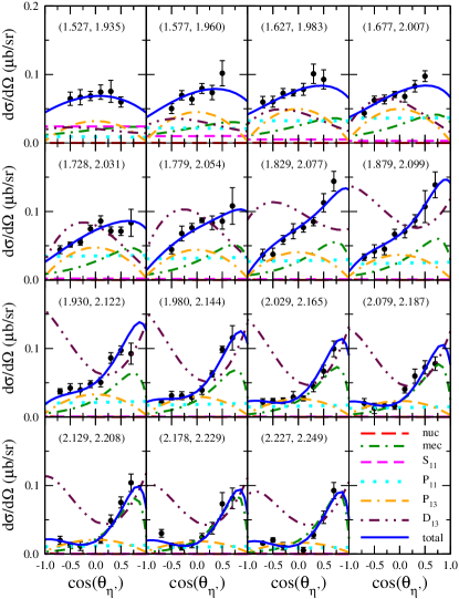
Figure 4: (Color online) Same as in Fig. 3 for the fit result of Table 2. The nucleonic current contribution (long-dashed curves) is very small and cannot be seen on the present scale.

Table 3: Same as Table 2. More resonances were added here to see whether this would further improve the fit. $\chi^{2}/N=1.04$.

Nucleonic current:
$g_{NN\eta^{\prime}}$	1.33
$\lambda$	0.0
$\Lambda_{N}$ (MeV)	1200
Mesonic current:
$g_{\eta^{\prime}\rho\gamma}$	1.25
$g_{\eta^{\prime}\omega\gamma}$	0.44
$\Lambda_{v}$ (MeV)	1515
$N^{*}=S_{11}$ current:
$m_{N^{*}}$ (MeV)	1539	1670	2025
$g_{NN^{*}\gamma}\,g_{NN^{*}\eta^{\prime}}$	-6.48	1.10	0.03
$\lambda$	0.78	0.93	0.07
$\Lambda_{N^{*}}$ (MeV)	1200	1200	1200
$\Gamma_{N^{*}}$ (MeV)	138	79	79
$\gamma_{N\gamma}$			0.001
$\beta_{N\pi}$	0.5	0.9	0.96
$\beta_{N\eta}$	0.5	0.1
$\beta_{N\eta^{\prime}}$			0.04
$N^{*}=P_{11}$ current:
$m_{N^{*}}$ (MeV)	1718	2099	2406
$g_{NN^{*}\gamma}\,g_{NN^{*}\eta^{\prime}}$	1.45	-0.90	-0.27
$\lambda$	1.00	0.78	0.71
$\Lambda_{N^{*}}$ (MeV)	1200	1200	bf1200
$\Gamma_{N^{*}}$ (MeV)	89	172	82
$\gamma_{N\gamma}$		0.002	0.002
$\beta_{N\pi}$	0.15	0.51	0.00
$\beta_{N\pi\pi}$	0.85
$\beta_{N\eta^{\prime}}$		0.49	1.00
$N^{*}=P_{13}$ current:
$m_{N^{*}}$ (MeV)	1943
$g_{1NN^{*}\gamma}\,g_{NN^{*}\eta^{\prime}}$	0.06
$g_{2NN^{*}\gamma}\,g_{NN^{*}\eta^{\prime}}$	-0.13
$\Lambda_{N^{*}}$ (MeV)	1200
$\Gamma_{N^{*}}$ (MeV)	109
$\gamma_{N\gamma}$	0.002
$\beta_{N\pi}$	0.59
$\beta_{N\omega}$	0.4
$\beta_{N\eta^{\prime}}$	0.01
$N^{*}=D_{13}$ current:
$m_{N^{*}}$ (MeV)	1782	2085
$g_{1NN^{*}\gamma}\,g_{NN^{*}\eta^{\prime}}$	-0.17	-0.01
$g_{2NN^{*}\gamma}\,g_{NN^{*}\eta^{\prime}}$	-0.24	0.10
$\Lambda_{N^{*}}$ (MeV)	1200	1200
$\Gamma_{N^{*}}$ (MeV)	152	141
$\gamma_{N\gamma}$		0.001
$\beta_{N\pi}$	0.1	0.97
$\beta_{N\pi\pi}$	0.9
$\beta_{N\eta^{\prime}}$		0.03

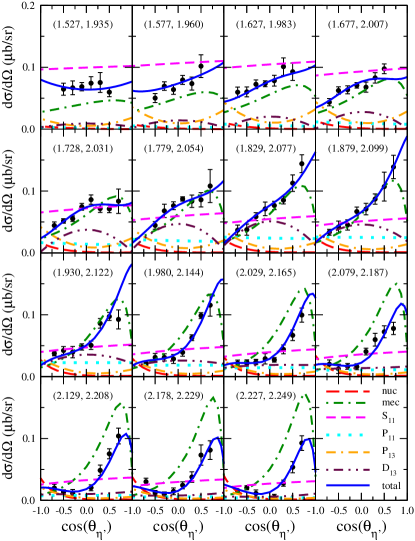
Figure 5: (Color online) Same as in Fig. 3 for the fit result of Table 3.

Table 4: Same as Table 1. No $P_{13}$ resonance was allowed here. $\chi^{2}/N=1.10$.

Nucleonic current:
$g_{NN\eta^{\prime}}$	0.002
$\lambda$	0.0
$\Lambda_{N}$ (MeV)	1200
Mesonic current:
$g_{\eta^{\prime}\rho\gamma}$	1.25
$g_{\eta^{\prime}\omega\gamma}$	0.44
$\Lambda_{v}$ (MeV)	1428
$N^{*}=S_{11}$ current:
$m_{N^{*}}$ (MeV)	1542	1848
$g_{NN^{*}\gamma}\,g_{NN^{*}\eta^{\prime}}$	-10.33	2.12
$\lambda$	1.00	1.00
$\Lambda_{N^{*}}$ (MeV)	1200	1200
$\Gamma_{N^{*}}$ (MeV)	233	164
$\beta_{N\pi}$	0.5	1.00
$\beta_{N\eta}$	0.5
$N^{*}=P_{11}$ current:
$m_{N^{*}}$ (MeV)	1710	1996
$g_{NN^{*}\gamma}\,g_{NN^{*}\eta^{\prime}}$	4.34	-1.37
$\lambda$	1.00	0.13
$\Lambda_{N^{*}}$ (MeV)	1200	1200
$\Gamma_{N^{*}}$ (MeV)	39	118
$\gamma_{N\gamma}$		0.002
$\beta_{N\pi}$	0.15	0.26
$\beta_{N\pi\pi}$	0.85
$\beta_{N\eta^{\prime}}$		0.74
$N^{*}=D_{13}$ current:
$m_{N^{*}}$ (MeV)	1756	2087
$g_{1NN^{*}\gamma}\,g_{NN^{*}\eta^{\prime}}$	-0.67	-0.08
$g_{2NN^{*}\gamma}\,g_{NN^{*}\eta^{\prime}}$	0.02	0.15
$\Lambda_{N^{*}}$ (MeV)	1200	1200
$\Gamma_{N^{*}}$ (MeV)	48	134
$\gamma_{N\gamma}$		0.002
$\beta_{N\pi}$	1.00	0.88
$\beta_{N\eta^{\prime}}$		0.12

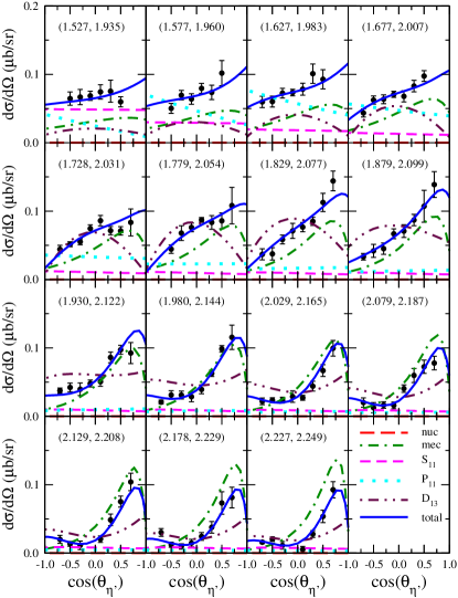
Figure 6: (Color online) Same as in Fig. 3 for the fit result of Table 4. The nucleonic current contribution (long-dashed curves) is negligible and cannot be seen on the present scale.

III.1 Differential cross sections

The details of the fits presented here are given in Tables 1–5 and the corresponding Figs. 3–7. For the purpose of easy comparison, Fig. 2 provides an overview of all those results. All five fits were obtained using the energy-dependent width functions of Sec. II.2. They all have comparable overall $\chi^{2}$ from each other and describe the data quite well. We see that most of the differences among them are at forward and backward angles where there are no data. Therefore, measurements of the cross sections at more forward and backward angles than presently available would disentangle some of the results in Fig. 2. Despite the fact that the overall quality of the fits is comparable to each other, the resulting parameter values are quite different. In particular, the fit set in Table 1 contains the minimum number of resonances (four) required to meet the present fit-quality criterium mentioned in the beginning of this section. In contrast to the analysis of the SAPHIR data NH1 , the inclusion of the spin-3/2 resonaces is important in order to reproduce the data quantitatively. As mentioned before, although we cannot identify the resonances uniquely in the present analysis, Table 1 reveals that one of the resulting resonances, $P_{11}(2104)$, is consistent with that quoted by the PDG PDG as one-star resonance. In the fit set of Table 2, we have included an additional $D_{13}$ resonance. Here, all the resonances but one are above the $\eta^{\prime}$ production threshold energy and that two of the resulting spin-3/2 resonances, $P_{13}(1900)$ and $D_{13}(2084)$, are consistent with those seen and quoted by the PDG PDG as two-star resonances. Also, in this particular set of parameters, the resulting $NN\eta^{\prime}$ coupling constant is very small. The fit set of Table 3 includes three $S_{11}$ and three $P_{11}$ resonances, instead of one each as in Table 2, keeping the number of spin-3/2 resonances unchanged compared to the fit set of Table 2. Here, two of the $S_{11}$, one of the $P_{11}$ and one of the $D_{13}$ resonances end up well below the production threshold, while one $P_{11}$ resonance mass is close to 2.4 GeV. With the exception of the latter resonance, all the resulting resonance masses are consistent with those quoted by the PDG PDG as four-star [$S_{11}(1535)$, $S_{11}(1650)$], three-star [$P_{11}(1710),D_{13}(1720)$], two-star [$P_{13}(1900)$, $D_{13}(2080)$], and one-star [$S_{11}(2090),P_{11}(2100)$] resonances. Here, the $NN\eta^{\prime}$ coupling constant is $g_{NN\eta^{\prime}}\approx 1.3$. In the fit result of Table 4, we have omitted the $P_{13}$ resonance and considered two $S_{11}$, three $P_{11}$ and two $D_{13}$ resonances. Again, three of the resulting resonances, $S_{11}(1538)$, $P_{11}(1710)$, and $D_{13}(2090)$, are consistent with known resonances. The $NN\eta^{\prime}$ coupling constant is practically zero, in line with the small value obtained for the fit result of Table 2. We have also considered all the known spin-1/2 and -3/2 resonances PDG (including those with only one star) in our fit. The resulting parameter values are displayed in Table 5. Here the resonance masses are fixed at the respective (centroid) values given in Ref. PDG . The resulting resonance widths are all consistent with those quoted in Ref. PDG . The $P_{11}(1440)$ resonance has practically no influence on the observables considered here and, therefore, it has been omitted in the fit set shown. For the $NN\eta^{\prime}$ coupling constant, we obtained $g_{NN\eta^{\prime}}=1.9$.

All these parameter sets illustrate the fact that cross sections do not impose enough constraints to the fit in order to extract definitive information on the resonances. Spin observables, on the other hand, do impose more stringent constraints and help distinguish among these parameter sets, as we shall show later.

Table 5: Same as Table 1. All resonance masses are kept at their PDG values. $\chi^{2}/N=1.01$.

Nucleonic current:
$g_{NN\eta^{\prime}}$	1.91
$\lambda$	0.0
$\Lambda_{N}$ (MeV)	1200
Mesonic current:
$g_{\eta^{\prime}\rho\gamma}$	1.25
$g_{\eta^{\prime}\omega\gamma}$	0.44
$\Lambda_{v}$ (MeV)	1447
$N^{*}=S_{11}$ current:
$m_{N^{*}}$ (MeV)	1535	1650	2090
$g_{NN^{*}\gamma}\,g_{NN^{*}\eta^{\prime}}$	-2.59	4.00	-0.07
$\lambda$	0.23	0.66	1.00
$\Lambda_{N^{*}}$ (MeV)	1200	1200	1200
$\Gamma_{N^{*}}$ (MeV)	101	197	62
$\gamma_{N\gamma}$			0.001
$\beta_{N\pi}$	0.5	0.9	0.04
$\beta_{N\eta}$	0.5	0.1
$\beta_{N\eta^{\prime}}$			0.96
$N^{*}=P_{11}$ current:
$m_{N^{*}}$ (MeV)	1710	2100
$g_{NN^{*}\gamma}\,g_{NN^{*}\eta^{\prime}}$	-3.87	-0.39
$\lambda$	0.27	0.14
$\Lambda_{N^{*}}$ (MeV)	1200	1200
$\Gamma_{N^{*}}$ (MeV)	249	75
$\gamma_{N\gamma}$		0.002
$\beta_{N\pi}$	0.15	0.50
$\beta_{N\pi\pi}$	0.85
$\beta_{N\eta^{\prime}}$		0.50
$N^{*}=P_{13}$ current:
$m_{N^{*}}$ (MeV)	1720	1900
$g_{1NN^{*}\gamma}\,g_{NN^{*}\eta^{\prime}}$	-0.44	0.04
$g_{2NN^{*}\gamma}\,g_{NN^{*}\eta^{\prime}}$	1.49	-0.54
$\Lambda_{N^{*}}$ (MeV)	1200	1200
$\Gamma_{N^{*}}$ (MeV)	107	316
$\beta_{N\pi}$	0.2	0.6
$\beta_{N\rho}$	0.8
$\beta_{N\omega}$		0.4
$N^{*}=D_{13}$ current:
$m_{N^{*}}$ (MeV)	1520	1700	2080
$g_{1NN^{*}\gamma}\,g_{NN^{*}\eta^{\prime}}$	-1.00	-0.92	-0.07
$g_{2NN^{*}\gamma}\,g_{NN^{*}\eta^{\prime}}$	0.46	0.95	0.08
$\Lambda_{N^{*}}$ (MeV)	1200	1200	1200
$\Gamma_{N^{*}}$ (MeV)	135	49	102
$\gamma_{N\gamma}$			0.001
$\beta_{N\pi}$	0.55	0.10	0.87
$\beta_{N\pi\pi}$	0.45	0.90
$\beta_{N\eta^{\prime}}$			0.13

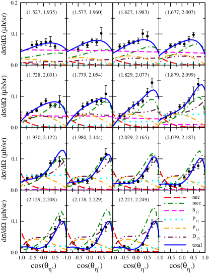
Figure 7: (Color online) Same as in Fig. 3 for the fit result of Table 5.

Although the parameter sets in Tables 1–5 yield comparable fits to the cross section, the corresponding dynamical contents are quite different from each other. Let us discuss, therefore, some of the different features present in the results corresponding to the various parameter sets. Figure 3 shows some details of the dynamical content of our model corresponding to the fit results given in Table 1. Here, both the $S_{11}$ and $P_{13}$ resonances have the largest contribution at low energies; the former dies out as the energy increases while the latter contribution persists to higher energies. The angular shape of the $P_{13}$ resonance current contribution is concave with a maximum at $\theta_{\eta^{\prime}}\approx 90^{\circ}$. The $P_{11}$ resonance contributes mostly around $T_{\gamma}=1.879$ GeV. Its angular shape is rather flat (note that it includes both the $s$- and $u$-channel contributions). However, its interference with other contributions, such as that due to the $S_{11}$ resonance, leads to a distinctive angular dependence. Although the $D_{13}$ resonance current is relatively small in this particular fit set, it plays an important role in reproducing the data through its interference with other currents. The mesonic current contribution plays a crucial role in reproducing the observed forward-peaked angular distribution, especially at higher energies. This is a general feature observed in many reactions at high energies where the $t$-channel mechanism (either Regge trajectories or meson exchanges) accounts for the small-$t$ behavior of the cross section. However, the present result shows also a competing mechanism due to resonances and that the observed forward-peaked angular distribution is a result of significant interference effects. We note that this feature is not restricted to the particular set of the parameter values of Table 1, but it is also found in other sets that fit the data (note, in particular, a relatively large $S_{11}$ resonance contribution in Fig. 5 and a $D_{13}$ resonance contribution in Figs. 4, 6 and 7 at higher energies). Therefore, this feature prevents us from fixing uniquely the mesonic current from the cross-section data at forward angles and higher energies. The nucleonic current contribution is very small here; however, as mentioned in the beginning of this section, the cross-section data alone do not impose stringent constraints on the fit so that it is possible to reproduce the data equally well with a much larger coupling constant, as can be seen in Tables 3 and 5. We will come back to this issue later, in Sec. III.3.

Figure 4 shows the dynamical content of our model corresponding to the fit results given in Table 2. Here, the $S_{11}$ resonance contribution is considerable only at the lowest energy measurement and already at $T_{\gamma}=1.627$ GeV, it becomes very small and it is practically negligible for higher energies. Both the $P_{11}$ and $P_{13}$ resonance contributions exhibit similar features to those observed in Fig. 3, with both contributions reaching its maximum around $T_{\gamma}=1.677$ GeV. The $D_{13}$ resonance contribution is large over the energy region considered, except at lower energies. Above $T_{\gamma}\approx 1.677$ GeV, it is the largest contribution. Its angular shape changes drastically with energy, starting with a small negative curvature in the lower energy region and ending with a roughly convex shape in the higher energy region. Note that this energy dependence of the angular shape is due to an interference between the two $D_{13}$ resonances with different masses. Although somewhat larger, the mesonic current contribution is essentially the same to that in Fig. 3. As has been pointed out above, there is a considerable interference effects between the mesonic and the ($D_{13}$) resonance currents at higher energies. The nucleonic current is practically zero in Fig. 4 since, as mentioned above, the resulting $NN\eta^{\prime}$ coupling constant is very small.

In the fit result of Table 3 shown in Fig. 5, the $S_{11}$ resonance contribution is very strong especially in the lower energy region and is quite appreciable even at higher energies. The $P_{11}$ resonance contribution basically shows the same feature as in the fit sets discussed above. The $P_{13}$ resonance contribution exhibits a convex angular shape, just opposite to the concave shape shown in Figs. 3 and 4. This difference is due to the relative sign difference between the coupling constants $g_{1NN^{*}\eta^{\prime}}$ and $g_{2NN^{*}\eta^{\prime}}$ as compared to the results shown in Figs. 3 and 4. The $D_{13}$ resonance contribution is largest around $T_{\gamma}=1.829$ GeV. The shape of the angular distribution is quite different from the other fit discussed above. Together with the $P_{13}$ resonance, it describes some of the details of the observed angular distribution around $T_{\gamma}=1.779$ GeV. The mesonic current is much larger in this fit than in the other fits. In particular, it largely overestimates the measured cross section in the higher energy region. Its destructive interference with the other currents brings down the total contribution in agreement with the data. Once more, this shows that one has to be cautious in trying to fix the $t$-channel contribution using the cross-section data at forward angles and higher energies. The nucleonic current gives an appreciable contribution in this fit, especially at higher energies and backward angles due to the $u$-channel. The corresponding $NN\eta^{\prime}$ coupling constant is $g_{NN\eta^{\prime}}=1.33$.

Figure 6 shows the dynamical content of the fit result of Table 4. The $S_{11}$ resonance contribution is largest at the lowest energy, but it decreases quickly as the energy increases. The $P_{11}$ resonance contribution is largest around $T_{\gamma}=1.627$ GeV, with more pronounced angular distribution than in the other fit results. The $D_{13}$ resonance contribution has a concave angular shape in the lower energy region and is largest at around $T_{\gamma}=1.829$ GeV. For higher energies the angular shape changes and gives the largest contribution for forward angles apart from the mesonic current, the latter providing again the bulk of the observed rise of the cross section at forward angles. The $P_{13}$ resonance is not included in this fit set. We note that, unlike in Fig. 5, some of the details of the observed angular distribution around $T_{\gamma}=1.779$ GeV is not well reproduced, indicating the importance of both the $P_{13}$ and $D_{13}$ resonances. The nucleonic current contribution is practically zero.

The dynamical content of the fit result given in Table 5 is shown in Fig. 7. Overall, except for the lower energies, the mesonic current yields the largest contribution. The $S_{11}$ and $P_{13}$ resonance contributions are important in the low energy region while the $P_{11}$, $P_{13}$, and $D_{13}$ resonances are important in the higher energy region. The nucleonic current is non-negligible only for backward angles at higher energies. Here, one major difference from the other fit results is the rather pronounced bending downward of the cross section (solid curves) for forward angles at lower energies. Measurements of the cross sections for more forward angles would tell us whether such a behavior would indeed be necessary.

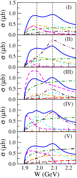
Figure 8: (Color online) Total cross section for $\gamma p\to p\eta^{\prime}$ as a function of the total energy of the system, $W=\sqrt{s}$. The panels from top to bottom correspond to the fit results of Tables 1–5, as indicated. The overall total cross sections (solid lines) are broken down according to their dynamical contributions, with line styles defined in Fig. 3. The two dashed vertical lines are placed to guide the eye through the two bump positions in all panels.

III.2 Total cross sections

Figure 8 shows the predictions for the total cross sections obtained by integrating the corresponding differential cross sections shown in Figs. 3-7. Although these predictions may suffer from considerable uncertainties due to differences in the corresponding differential cross sections, especially at lower energies, they exhibit a common feature, i.e., the total cross sections (solid curves) seems to show a bump structure around $W=2.09$ GeV which is caused mainly by the $P_{11}$ and/or $D_{13}$ resonance depending on the fit set. Note that the PDG quotes a two-star $D_{13}(2080)$ and a one-star $P_{11}(2100)$ resonance which are practically at this bump position. There is also a one-star resonance, $S_{11}(2090)$, that is just at the bump and, therefore, might have contributed to its structure. However, the angular distribution does not favor this possibility. The total cross section also seems to exhibit a bump structure at a lower energy of around $W=1.96$ GeV due to the $S_{11}$, $P_{11}$ and/or $P_{13}$ resonance depending on the fit set. The latter two resonances can also contribute to the broadening of this bump depending on the fit set, as can be seen in Fig. 8. A rather sharp rise of the cross section from the threshold is caused by the $S_{11}$ resonance, except in the top two panels, where the $P_{13}$ resonance also contributes to this rise. The structures exhibited by the total cross section, in particular the bump around $W=2090$ GeV, are unlikely to be artifacts of the present predictions and, consequently, we would expect them to show up in the actual total cross-section data when they are measured.

III.3 $NN\eta^{\prime}$ coupling constant

As we have seen in this section, unfortunately the present analysis cannot determine the $NN\eta^{\prime}$ coupling constant, since the available cross-section data can be reproduced equally well with different sets of parameters in which this coupling constant varies considerably. However, an upper limit of its value can still be estimated. One of the reasons why $g_{NN\eta^{\prime}}$ cannot be extracted uniquely from the cross-section data is that the resonance currents, especially the one due to the $D_{13}$ resonance, can give rise to the observed enhancement of the backward-angle cross section as shown in Figs. 4 and 6. Also, the $P_{11}$ resonance current alone can lead to a feature of the cross section similar to that due to the nucleonic current, i.e., the enhancement of the backward-angle cross section at higher energies through the $u$-channel contribution. The resonance currents can also interfere destructively with the nucleonic current in which case one obtains a larger $NN\eta^{\prime}$ coupling constant. In fact, in a very extreme case, we have obtained a fit value as large as $g_{NN\eta^{\prime}}=3.0$. It is obvious, therefore, that a more unambiguous extraction of this coupling constant requires going to an energy region where the resonance contributions are small. Figure 9 illustrates this point; here we show the fit result considering the data with energies at $T_{\gamma}=2.129$ GeV and above only and assuming a scenario in which no resonance currents contribute at these energies. The resulting fit parameters are $g_{NN\eta^{\prime}}=2.10$ for the $NN\eta^{\prime}$ coupling constant and $\Lambda_{v}=1264$ MeV for the cutoff parameter in the form factor at the $\eta^{\prime}v\gamma$ vertex. In Fig. 9 we see that the nucleonic and mesonic currents interfere with each other. However, the interference pattern is such that it does not cause any problem in fixing both the nucleonic and mesonic current contributions to a large extent. In any case, judging from the overall results of our analysis, we would not expect $g_{NN\eta^{\prime}}$ to be much larger than 2.

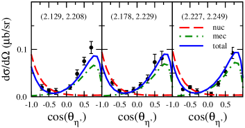
Figure 9: (Color online) Fit result with no resonances. $g_{NN\eta^{\prime}}=2.10$ and $\Lambda_{v}=1264$ MeV. See caption of Fig. 4.

III.4 Meson exchanges versus Regge trajectory

It is well known that $t$-channel processes at high energies (above $\sim$3–5 GeV) may also be described by Regge trajectories. However, how far down in energy one can go with this description before an explicit inclusion of ordinary meson exchange is required is still an open issue. We would expect a smooth transition from a description in terms of meson exchanges to one in terms of Regge trajectory as one goes up higher in energy. The issue of meson exchanges versus Regge trajectory is particularly relevant in the present context, for the extracted resonance parameters can depend on these two alternatives for modeling the $t$-channel contribution NH1 .

In their analysis of the SAPHIR data SAPHIR , Chiang et al. Chiang advocate the use of Regge trajectories while other authors others have employed vector-meson exchanges. In our previous analysis of these data, we found NH1 that they can be reproduced equally well using either meson exchanges (with form factors at the $v\eta^{\prime}\gamma$ vertices) or a Regge trajectory for the $t$-channel contribution. It is interesting to see whether the same is true for the new CLAS data CLAS . We have repeated the calculation with the Regge trajectory following Ref. NH1 . In particular, we replace the $t$-channel meson exchange propagators by the corresponding Regge trajectories keeping everything else unchanged, except that the form factor at the $v\eta^{\prime}\gamma$ vertex is set to unity. All the free parameters of the model are refitted again. We found that the fit quality using the Regge trajectory is, at best, comparable to that obtained using the ordinary meson exchanges for the $t$-channel. For example, the $\chi^{2}$ corresponding to the fit set of Table 2 is $\chi^{2}/N=1.17$ compared to $\chi^{2}/N=1.04$ obtained with explicit meson exchanges; for the fit set of Table 5, the Regge-trajectory result is $\chi^{2}/N=1.08$, as compared to $\chi^{2}/N=1.01$ using meson exchanges. Similar results are obtained for other fit sets considered in subsection III.A.

III.5 Spin observables

We now turn our attention to spin observables. As we have shown in Fig. 2, cross sections do not impose very severe constraints on the model parameter values. We expect spin observables to be more sensitive in this respect. The predictions for the beam and target asymmetries corresponding to the fit results of Tables 1–5 are shown in Fig. 10. As we can see, unlike the cross sections (see Fig. 2), the predictions vary considerably between the different parameter sets. For energies where the beam asymmetry is less sensitive to the parameter sets, the target asymmetry is quite sensitive and vice versa. Therefore, overall, a combined analysis of these spin observables will impose much more stringent constraints on the fit and should help determine better the model parameters.

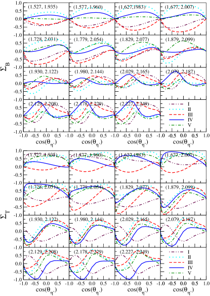
Figure 10: (Color online) Photon beam and target nucleon asymmetries $\Sigma_{B}$ (top panel) and $\Sigma_{T}$ (bottom), respectively, for $\gamma p\to p\eta^{\prime}$ as a function of the $\eta^{\prime}$ emission angle $\theta_{\eta^{\prime}}$ in the center-of-momentum system. See the caption of Fig. 2 for the meaning of the different curves.

IV Summary

We have analyzed the new CLAS CLAS data of the $\gamma p\to p\eta^{\prime}$ reaction within an approach based on a relativistic meson-exchange model of hadronic interactions. The present model is an extension of the one reported in Ref. NH1 and it includes the nucleonic and the mesonic as well as the nucleon-resonance currents. The latter includes both spin-1/2 and -3/2 resonance contributions in contrast to our previous work NH1 , where only spin-1/2 resonances were considered. In addition, we employ energy-dependent resonance widths in the present work. The resulting reaction amplitude is fully gauge invariant.

We have shown that the mesonic as well as the spin-1/2 and -3/2 resonance currents are important to describe the existing data quantitatively. The observed angular distribution is due to delicate interference effects between the different currents. In our analysis, most of the resulting resonances may be identified with known resonances PDG . We emphasize, however, that one should be cautious with such an identification of the resonances. As we have seen, the cross-section data alone do not impose enough constraints for an unambiguous determination of the resonance parameters. In this connection, we have shown that the beam and target asymmetries can help impose more stringent constraints. Furthermore, there is a possibility that some of the resonances in the present work are mocking up background contributions, especially those due to the final-state interaction, which is not taken into account explicitly in our calculation. Obviously, effects of the final-state interaction should be investigated in future work before a conclusive identification of the resonances can be made.

We have predicted a bump structure in the total cross section at $W\approx 2.09$ GeV (see Fig. 8). If this is confirmed, the $D_{13}(2080)$ and/or $P_{11}(2100)$ resonance may be responsible for this bump.

Our study also shows that the nucleonic current should be relatively small. However, contrary to the expectation in our earlier work NH1 , the new high-precision cross-section data do not allow to pin down this current contribution due to the possible presence of resonance currents, especially of the $D_{13}$ resonance, which can also lead to an enhancement of the cross section for backward angles at higher energies, a feature that otherwise arises from the $u$-channel nucleonic current contribution. These complications notwithstanding, assuming that for the very high end of the present data set resonance contributions can be neglected, we argue in Sec. III.3 that the upper limit of $g_{NN\eta^{\prime}}$ can now be lowered to a value of $g_{NN\eta^{\prime}}\lesssim 2$, whereas our previous analysis NH1 had suggested an upper limit of $g_{NN\eta^{\prime}}\lesssim 3$. Further corroboration of this finding is needed.

In this respect, it should be noted that the result pertaining here to the $NN\eta^{\prime}$ coupling constant is, of course, a model-dependent one. Indeed, what is relevant in our calculations is the product of $g_{NN\eta^{\prime}}$ and the associated hadronic form factor which accounts for the off-shellness of the intermediate nucleon. Moreover, our $NN\eta^{\prime}$ coupling constant is defined at the on-mass-shell point, i.e., $g_{NN\eta^{\prime}}=g_{NN\eta^{\prime}}(q^{2}=m_{\eta^{\prime}}^{2})$ while the coupling required in Eq. (1) in connection with the origin of the nucleon spin is at $q^{2}=0$. Since the $\eta^{\prime}$ meson is a relatively heavy meson ($m_{\eta^{\prime}}\approx 957$ MeV), we would expect that $g_{NN\eta^{\prime}}(q^{2}=0)$ will be considerably smaller than its value at $q^{2}=m_{\eta^{\prime}}^{2}$ because of the presence of the form factor which usually cut down the coupling strength. Therefore, we might well expect that the $NN\eta^{\prime}$ coupling at $q^{2}=0$ to be negligibly small, consistent with zero.

We have also shown that the mesonic current contribution cannot be fixed unambiguously from the existing cross-section data because of the possible presence of the resonance currents, especially the $D_{13}$ resonance. A possibility to determine the $t$-channel current is to measure the cross sections at higher energies where the resonance contributions becomes negligible.

Furthermore, we have found that using a Regge trajectory in the $t$-channel instead of explicit meson exchanges yields overall fit qualities that are, at best, comparable to those obtained with meson exchanges. This indicates that explicit $\rho$ and $\omega$ exchanges, as employed here, are completely adequate to describe the $t$-channel degrees of freedom at the present energies.

Finally, the results of the present work should provide useful information for further investigations, both experimentally and theoretically, of the $\gamma N\to N\eta^{\prime}$ reaction. In particular, measurements of cross sections at smaller forward and larger backward angles than are available in the present data set would already help constrain the model parameters considerably, as can be seen in Fig. 2. Total cross sections should also be measured in order to confirm or dismiss the bump structures, especially around $W=2.09$ GeV, predicted in the present calculation. In addition, it is expected that measurements of spin observables — such as beam and target asymmetries shown in Fig. 10 — would impose more stringent limits on the range of permissible parameters and this would undoubtedly provide a much improved description of the resonances and their properties in the energy region covered by the existing data. From the theoretical side, it is possible that the nucleon resonances introduced in the present work are mocking up the background contributions not taken into account in the calculation. In this connection, it is extremely interesting to investigate effects of the final-state interaction which has not been treated explicitly in the present calculation. Unfortunately, at present no realistic model is available that can provide the relevant $\eta^{\prime}N$ final-state interaction. In addition, effects of higher-spin resonances that have been ignored in the present analysis should be investigated in the future.

Appendix A Spin-3/2 Resonance Propagator

We employ here the Rarita–Schwinger (RS) choice for the free Lagrangian of a spin-3/2 particle with mass $m$,

$$\mathcal{L}=\bar{\psi}_{\mu}\Lambda^{\mu\nu}\psi_{\nu}~{},$$ (17)

where

$$\Lambda^{\mu\nu}=-\frac{i}{2}\left[\sigma^{\mu\nu},({p\!\!\!/}-m)\right]_{+}~{},$$ (18)

with $p=i\partial$, the anticommutator bracket $[a,b]_{+}=ab+ba$, and $\sigma^{\mu\nu}=\frac{i}{2}(\gamma^{\mu}\gamma^{\nu}-\gamma^{\nu}\gamma^{\mu})$. (In the RS choice, the parameter $A$ that usually appears in $\mathcal{L}$ is taken as $A=-1$ RSprop .) From

$$\Lambda_{\mu\lambda}S^{\lambda\nu}=S_{\mu\lambda}\Lambda^{\lambda\nu}=g_{\mu}^{\;\nu}~{},$$ (19)

the propagator is then found as

$$S^{\mu\nu}(p)=\frac{({p\!\!\!/}+m)\Delta^{\mu\nu}}{p^{2}-m^{2}}=\frac{\tilde{\Delta}^{\mu\nu}({p\!\!\!/}+m)}{p^{2}-m^{2}}~{},$$ (20)

where $\Delta^{\mu\nu}$ is the RS tensor of Eq. (7) (with $m=m_{R}$) and

$$\tilde{\Delta}^{\mu\nu}=-g^{\mu\nu}+\frac{1}{3}\gamma^{\mu}\gamma^{\nu}+\frac{2p^{\mu}p^{\nu}}{3m^{2}}-\frac{\gamma^{\mu}p^{\nu}-p^{\mu}\gamma^{\nu}}{3m}~{},$$ (21)

which differs from (7) by the sign of the last term.

When seeking an ansatz for describing a spin-3/2 resonance, we note first that there are, of course, infinitely many ways to achieve a pole description whose on-shell behavior on the real axis corresponds to replacing the mass of the elementary propagator by

$$m\to m_{R}-i\frac{\Gamma_{R}}{2}~{},$$ (22)

where $m_{R}$ is the resonance mass and $\Gamma_{R}$ the associated width. In constructing a resonant propagator, we are guided by the following motivation. As in the spin-1/2 case of (5), we want to describe the spin in terms of the elementary operators, i.e., we want to preserve the numerator structure of (20) and the symmetry between the RS tensors $\Delta$ and $\tilde{\Delta}$. In a schematic matrix notation, we therefore make the ansatz

$$S=X^{-1}({p\!\!\!/}+m)\Delta=\tilde{\Delta}({p\!\!\!/}+m)\tilde{X}^{-1}~{},$$ (23)

putting, in analogy to the denominator of the spin-1/2 case (5),

$$X =(p^{2}-m_{R}^{2})g+iA({p\!\!\!/}+m_{R})~{},$$ (24a)

$$\tilde{X} =(p^{2}-m_{R}^{2})g+i({p\!\!\!/}+m_{R})\tilde{A}~{},$$ (24b)

with the operators $A$ and $\tilde{A}$ to be determined such that the second equality in (23) holds true, i.e.,

$$X^{-1}({p\!\!\!/}+m)\Delta=\tilde{\Delta}({p\!\!\!/}+m)\tilde{X}^{-1}~{}.$$ (25)

Multiplying this equation by $\Lambda$ from both sides, one immediately finds the condition

$$({p\!\!\!/}+m_{R})\tilde{A}\Lambda=\Lambda A({p\!\!\!/}+m_{R})~{}.$$ (26)

In view of Eq. (19) and the fact that on-shell, at $p^{2}=m_{R}^{2}$ and acting on a spin-3/2 eigenstate, the propagator must provide the width information, we find that the ansatz

$$\tilde{A}^{\mu\nu}=-\Delta^{\mu\nu}\frac{\Gamma}{2}\quad\text{and}\quad A^{\mu\nu}=-\tilde{\Delta}^{\mu\nu}\frac{\Gamma}{2}~{},$$ (27)

satisfies all constraints. $\Gamma$ here may be any conveniently chosen width function that goes to the static width $\Gamma_{R}$ at the resonance mass $m_{R}$. We thus have

$$S(p)=\left[({p\!\!\!/}-m_{R})g-i\frac{\Delta}{2}\Gamma\right]^{-1}\Delta$$ (28a)

or

$$S(p)=\tilde{\Delta}\left[({p\!\!\!/}-m_{R})g-i\frac{\tilde{\Delta}}{2}\Gamma\right]^{-1}~{}.$$ (28b)

By construction, both forms are completely equivalent, similar to the equivalence of both forms for the elementary propagator (20).

The inversion here is to be performed on the full 16-dimensional space of Lorentz indices and component indices. There are various equivalent ways to do this; we have done it by introducing indices

$$i=4\mu+\beta\quad\text{and}\quad j=4\nu+\alpha~{},$$ (29)

where $\mu,\nu=0,1,2,3$ are the Lorentz indices and $\beta,\alpha=1,2,3,4$ are the component indices, and defining $16\times 16$ numerator and denominator matrices by

$$N_{ij} =\Delta^{\mu\lambda}_{\beta\alpha}g_{\lambda\nu}$$

$$=-\delta_{\mu\nu}\delta_{\beta\alpha}+\frac{2p^{\mu}p_{\nu}}{3m_{R}^{2}}\delta_{\beta\alpha}$$

$$\qquad\mbox{}+\left(\frac{1}{3}\gamma^{\mu}_{\beta\varepsilon}\gamma^{\lambda}_{\varepsilon\alpha}+\frac{\gamma^{\mu}_{\beta\alpha}p^{\lambda}-p^{\mu}\gamma^{\lambda}_{\beta\alpha}}{3m_{R}}\right)g_{\lambda\nu}$$ (30)

and

$$D_{ij}=p_{\lambda}\gamma^{\lambda}_{\beta\alpha}\delta_{\mu\nu}-m_{R}\delta_{\mu\nu}\delta_{\beta\alpha}-iN_{ij}\frac{\Gamma}{2}~{},$$ (31)

respectively. Numerically inverting the denominator matrix $D$, we then calculate the spin-3/2 propagator as

$$S^{\mu\nu}_{\beta\alpha}=\left(D^{-1}N\right)_{ik}g^{\rho\nu}~{},$$ (32)

where $k=4\rho+\alpha$ and summation over $\rho$ is implied, as usual.

References

- (1) S. Capstick and N. Isgur, Phys. Rev. D 34, 2809 (1986); S. Capstick and W. Roberts, ibid. 47, 1994 (1993); 49, 4570 (1994); 57, 4301 (1998); 58, 074011 (1998).
- (2) J. Ashman et al., Phys. Lett. B206, 364 (1988).
- (3) G. M. Shore and G. Veneziano, Nucl. Phys. B381, 23 (1992).
- (4) T. Hatsuda, Nucl. Phys. B329, 376 (1990); A. V. Efremov, J. Soffer, and N. A. Törnqvist, Phys. Rev. Lett. 64, 1495 (1990); Phys. Rev. D 44, 1369 (1991).
- (5) G. M. Shore and G. Veneziano, Phys. Lett. B244, 75 (1990).
- (6) T. Feldmann, Int. J. Mod. Phys. A15, 159 (2000).
- (7) S. Okubo, Phys. Lett. 5, 165 (1963); G. Zweig, CERN Report No. TH412, 1964; J. Iizuka, Prog. Theor. Phys. Suppl. 37–38, 21 (1966).
- (8) D. Adams et al., Phys. Rev. D56, 5330 (1997).
- (9) G. Altarelli and G. G. Ross, Phys. Lett. B212, 391 (1988); R. D. Carlitz, J. C. Collins, and A. H. Müller, ibid. B214, 229 (1988).
- (10) K. Nakayama and H. Haberzettl, Phys. Rev. C 69, 065212 (2004).
- (11) M. Dugger et al. (CLAS collaboration), nucl-ex/0512019.
- (12) R. Plötzke et al., Phys. Lett. B444, 555 (1998); J. Barth et al., Nucl. Phys. A691, 374c (2001).
- (13) H. Haberzettl, Phys. Rev. C 56, 2041 (1997).
- (14) H. Haberzettl, C. Bennhold, T. Mart, and T. Feuster, Phys. Rev. C 58, R40 (1998).
- (15) R. M. Davidson and R. Workman, Phys. Rev. C 63, 025210 (2001).
- (16) R. L. Walker, Phys. Rev. 182, 1729 (1969).
- (17) R. A. Arndt, R. L. Workman, Z. Li, and L. D. Roper, Phys. Rev. C 42, 1864 (1990).
- (18) A. I. L’vov, V. A. Petrun’kin, and M. Schumacher, Phys. Rev. C 55, 359 (1997).
- (19) D. Drechsel, O. Hanstein, S. S. Kamalov, and L. Tiator, Nucl. Phys. A645, 145 (1999) [nucl-th/9807001].
- (20) Particle Data Group, Phys. Lett. B592, 1 (2004).
- (21) W. T. Chiang, S. N. Yang, L. Tiator, M. Vanderhaegen, and D. Drechsel, Phys. Rev. C 68, 045202 (2003).
- (22) B. Borasoy, Eur. Phys. J. A9, 95 (2000); B. Borasoy, E. Marco, and S. Wetzel, Phys. Rev. C 66, 055208 (2002); A. Sibirtsev, Ch. Elster, S. Krewald, and J. Speth, nucl-th/0303044.
- (23) P. A. Moldauer and K. M. Case, Phys. Rev. 102, 279 (1956); C. Fronsdal, Nuovo Cimento Suppl. 9, 416 (1958); A. Aurelia and H. Umezawa, Phys. Rev. 182, 1682 (1969); L. M. Nath, B. Etemadi, and J. D. Kimel, Phys. Rev. D 3, 2153 (1971); M. Benmerrouche, R. M. Davidson, and N. C. Mukhopadhyay, Phys. Rev. C 39, 2339 (1989).