Correlations between $\theta_{13}$ and $\theta_{23}$ in a very long baseline neutrino oscillation experiment

Abstract

A very long baseline experiment, with $L/E$ of $1.6\times 10^{4}$ m/MeV, has been proposed as the ideal means to measure $\theta_{13}$, including its sign, for neutrino energies less than 50 MeV. Higher energies require consideration of the earth MSW effect. Approximating a constant density mantle, we examine the $\nu_{e}$–$\nu_{\mu}$ and $\nu_{\mu}$–$\nu_{\mu}$ oscillation channels at very long baselines with particular focus upon the deviation of $\theta_{23}$ from maximal mixing and the sign of $\theta_{13}$. It is demonstrated that measurements of these oscillation channels in this region are sensitive to $\theta_{13}$, including its sign, and to $\theta_{23}$, including its octant, with a significant correlation between the value of $\theta_{13}$ and the difference of $\theta_{23}$ from maximal mixing.

I Introduction

All existing neutrino experiments (except the LSND lsnd appearance experiment) can be understood within the context of three-flavor neutrino oscillations. By relating three mass eigenstates to the flavor states via a unitary transformation parameterized in the canonical manner pdg , one has six free parameters with which to fit the experimental data: two mass-squared differences, three mixing angles, and one Dirac CP phase. Solar neutrino experiments solar along with KamLAND kamland point to the large mixing angle MSW solution with a mass-squared difference $\Delta_{21}\sim 8\times 10^{-5}$ eV² (with $\Delta_{jk}:=m_{j}^{2}-m_{k}^{2}$) and mixing angle $\theta_{12}\sim 0.58$. The results of the Super-Kamiokande atmospheric neutrino experiment superk , in addition to the K2K experiment k2k , indicate another mass scale with $\Delta_{31}\sim 2\times 10^{-3}\mathrm{eV}^{2}$ and a near maximal mixing angle $\theta_{23}\sim 0.79$. To date, of the reactor experiments, data from CHOOZ provide the most stringent limit on the magnitude of the remaining mixing angle $|\theta_{13}|<0.22$ at 90% CL for $\Delta_{31}=2\times 10^{-3}\mathrm{eV}^{2}$ chooz . No information is known about the level of CP violation in the neutrino sector; hence, there are no limits on the phase $\delta$. Recent analyses can be found in Refs. MSTV ; BGP and recent reviews in Refs. bargerrev ; neutreview ; BP ; BK .

A high-priority goal of the neutrino physics community is to more precisely determine the value of $\theta_{13}$. Future reactor experiments have been proposed to improve upon the CHOOZ results with the hope of establishing a lower bound on the magnitude of this mixing angle reactor . Measuring electron neutrino disappearance from a reactor yields a clean measurement of $\sin^{2}\theta_{13}$; however, this measurement cannont contribute to determining the sign of the angle. In order to reduce the systematic error, these experiments will have a near and far detector. An increase in sensitivity to $\sin^{2}\theta_{13}$ can be achieved by an innovative use of the near detector sergio1 . In addition, for atmospheric neutrinos traveling through the earth, the ratio of multi-GeV $e$-like to $\mu$-like fluxes is sensitive to $\sin^{2}\theta_{13}$ as well as the mass hierarchy sergio2 . Multi-GeV atmospheric neutrinos can also provide information on $\sin^{2}\theta_{13}$ and the hierarchy question through a measurement of the difference between $\mu^{+}$ and $\mu^{-}$ events sergio3 ; DIMVNM . Such a measurement would require an iron calorimeter detector such as the MINOS detector minos .

We are particularly interested in measurements that are sensitive to terms in the oscillation probabilities which are linear in $\sin\theta_{13}$. It is possible that experiments designed to focus upon such measurements might further reduce the errors on the value of $\theta_{13}$. In addition, other information about the mixing angle can be garnered from these measurements. We adopt the choice of bounds on the mixing angles and CP phase as proposed in Ref. angles . In contrast to the standard convention, this choice restricts the CP phase to $0\leq\delta<\pi$ while extending one mixing angle to negative values $-\pi/2\leq\theta_{13}\leq\pi/2$. The advantage is that the parameter space is a connected region whenever one takes CP to be conserved. Given this choice, it is clear that terms in the oscillation probability which are linear in $\sin\theta_{13}$ can aid in determining the sign of this mixing angle.

The exact expressions for the oscillation probabilities necessarily exhibit terms linear in $\sin\theta_{13}$ bargerrev ; however, given that oscillations occur at two different mass scales, most current experiments can be understood to a good approximation within the context of modified two-neutrino oscillations. In Ref. expansion , one finds perturbative expansions about the small quantities $\theta_{13}$ and/or the ratio of the mass-squared differences $\alpha:=\Delta_{21}/\Delta_{31}\sim 0.03$. From these expansions, we note that terms linear in $\theta_{13}$ are supressed by a factor of $\alpha$. Clearly, this small mixing angle will be of little consequence whenever this perturbative expansion is valid. Whenever oscillations due to the small mass-squared difference interferes with oscillations due to the large mass squared difference, the expansion is no longer a good approximation at low orders expansion . In terms of the baseline $L$ and neutrino energy $E$, these subdominant oscillations need to be considered whenever $L/E\gtrsim 10^{4}$ m/MeV.

The sub-GeV sample of atmospheric neutrinos in the Super-K experiment contains such baselines superk . The implications of these subdominant oscillations for the analysis of atmospheric neutrinos has been thoroughly investigated in Ref. smirnov1 . Terms linear in $\theta_{13}$, in part, could explain a possible excess of $e$-like events in the Super-K data. Earlier work examined this excess but in the absence of the linear terms eexcess . Additionally, in Ref. CGMM , a full three neutrino analysis of the atmospheric data is presented. In this work, the authors assume CP conservation; as they allow only positive $\theta_{13}$, they must consider two CP phases $\delta=0,\pi$. Relating this to our choice, negative $\theta_{13}$ corresponds to $\delta=\pi$. Small differences between the two choices of the CP phase are a direct result of the terms linear in $\sin\theta_{13}$. Finally, in the analyses presented in th13exp ; us , the authors note a small asymmetry in $\chi^{2}$ about $\theta_{13}=0$ attributable to such linear terms. Though statistically insignificant, two local minima in $\chi^{2}$ were found, one for positive $\theta_{13}$ and one negative.

In Ref. th13exp , it was determined, in vacuo, that the $\nu_{e}$–$\nu_{\mu}$ and $\nu_{\mu}$–$\nu_{\mu}$ oscillation channels exhibited signficant linear dependence upon $\theta_{13}$ whenever one had a baseline-energy ratio of $L/E=2(2n+1)\pi/\Delta_{12}$. With $n=0$, the first $\Delta_{21}$ oscillation trough, a twenty-five percent effect was found on the $\nu_{\mu}$–$\nu_{\mu}$ channel for the presently allowed range of $\theta_{13}$. This ideal baseline is $L/E=1.6\times 10^{4}$ m/MeV.

A purpose of this work is to extend the results of Ref. th13exp to include the MSW effect msw so that one may employ higher energy neutrinos to probe the region of interest cited above. We show herein that even with higher energy neutrinos an experiment which is sensitive to linear terms in $\theta_{13}$ is still beyond present technology but perhaps more feasible. We also examine the correlation between the value of $\theta_{13}$ and the deviation of $\theta_{23}$ from maximal mixing. We take as known all parameters but these two mixing angles; granted, a full consideration of all parameters can have significant impact upon such correlations freund . We first consider vacuum oscillations which showcase the essential feautres. In the subsequent section, we permit matter interactions via the MSW effect. An approximate analytical expression is derived to demonstrate the relation between the two mixing angles. The general features found in the vacuum analysis remain. We then examine through numerical means the implications of the results for designing the ideal experiment that would be most sensitive to terms linear in $\theta_{13}$. Finally, we note that two existing three-neutrino analyses ggth23 ; ggpostks might demonstrate the correlation between $\theta_{13}$ and $\theta_{23}$.

II Vacuum oscillations

We shall assume CP is conserved. This assumption is indeed significant as all terms in the oscillation probabilities which are linear in $\sin\theta_{13}$ will be modulated by either $\cos\delta$ or $\sin\delta$. Thus if CP is violated, our results will be modified at the quantitative level. However, in the absence of any evidence for CP violation in the neutrino sector, we will default to the simplest case of no violation.

In vacuo, the relativistic limit of the neutrino evolution equation in the flavor basis is

$$i\partial_{t}\nu_{f}=\frac{1}{2E}U\mathcal{M}U^{\dagger}\nu_{f}$$ (1)

for neutrino energy $E$, mixing matrix $U$, and mass-squared matrix $\mathcal{M}=\mathrm{diag}(0,\Delta_{21},\Delta_{31})$. This first order differential equation is easily solved to give explicit expressions for the oscillation probabilities. The probability that a neutrino of flavor $\alpha$ will be detected a distance $L$ from the source as a neutrino of flavor $\beta$ is

$$\mathcal{P}_{\alpha\beta}(L/E)=\delta_{\alpha\beta}-4\sum^{3}_{\genfrac{}{}{0.0pt}{}{k<j}{j,k=1}}(U_{\alpha j}U_{\alpha k}U_{\beta k}U_{\beta j})\sin^{2}{\varphi_{jk}}$$ (2)

with $\varphi_{jk}:=\Delta_{jk}L/4E$. As we are interested in the oscillatory region for the small mass-squared difference $\Delta_{21}$, we will assume that the oscillations due to the two larger mass-squared differences are incoherent; that is, we take

$$\langle\sin^{2}{\varphi_{31}}\rangle=\langle\sin^{2}{\varphi_{32}}\rangle=\frac{1}{2}.$$ (3)

The $\nu_{e}$–$\nu_{e}$ oscillation channel exhibits no linear dependence on $\sin{\theta_{13}}$, so we neglect it in our analysis. Using the shorthand notation $s_{jk}:=\sin{\theta_{jk}}$ and $c_{jk}:=\cos{\theta_{jk}}$, the interesting oscillation channels in the prescribed limit become

$$\mathcal{P}_{e\mu} = [\tfrac{1}{2}\sin{2\theta_{12}}\cos{2\theta_{12}}\sin{2\theta_{13}}c_{13}\sin{2\theta_{23}}$$ (4)

$$+\sin^{2}{2\theta_{12}}c_{13}^{2}(c_{23}^{2}-s_{13}^{2}s_{23}^{2})]\sin^{2}{\varphi_{12}}$$

$$+\tfrac{1}{2}\sin^{2}{2\theta_{13}}s_{23}^{2},$$

$$\mathcal{P}_{\mu\mu} = 1-[\cos^{2}{2\theta_{12}}s_{13}^{2}\sin^{2}{2\theta_{23}}$$ (5)

$$+2\sin{2\theta_{12}}\cos{2\theta_{12}}s_{13}\sin{2\theta_{23}}(c_{23}^{2}-s_{13}^{2}s_{23}^{2})$$

$$+\sin^{2}{2\theta_{12}}(c_{23}^{2}-s_{13}^{2}s_{23}^{2})^{2}]\sin^{2}{\varphi_{12}}$$

$$-2c_{13}^{2}s_{23}^{2}(1-c_{13}^{2}s_{23}^{2}),$$

$$\mathcal{P}_{\mu\tau} = [-\sin^{2}{2\theta_{12}}(c_{23}^{2}-s_{13}^{2}s_{23}^{2})(s_{23}^{2}-s_{13}^{2}c_{23}^{2})$$ (6)

$$+\sin{2\theta_{12}}\cos{2\theta_{12}}s_{13}(1+s_{13}^{2})\sin{2\theta_{23}}\cos{2\theta_{23}}$$

$$+\cos^{2}{2\theta_{12}}s_{13}^{2}\sin^{2}{2\theta_{23}}]\sin^{2}\varphi_{12}$$

$$+\tfrac{1}{2}c_{13}^{4}\sin^{2}{2\theta_{23}}.$$

As stated, for the mass-squared difference $\Delta_{31}=2\times 10^{-3}$, the results of CHOOZ chooz restrict the magnitude of $\theta_{13}$ by

$$|\theta_{13}|<0.22\qquad(90\%~{}\mathrm{C.L.}).$$ (7)

Additionally, an analysis ggth23 which aims to determine the octant of $\theta_{23}$ indicates a range

$$0.67<\theta_{23}<0.91\qquad(90\%~{}\mathrm{C.L.}).$$ (8)

Permitting negative values of $\theta_{13}$, the allowed deviation of $\theta_{13}$ from zero is on the same order of magnitude as the allowed deviation of $\theta_{23}$ from maximal mixing. We introduce the parameter $\varepsilon$ to indicate the octant of $\theta_{23}$ via

$$\theta_{23}=\frac{\pi}{4}+\varepsilon$$ (9)

so that negative (positive) $\varepsilon$ indicates that $\theta_{23}$ is in the first (second) octant.

We expand the in vacuo oscillation probabilities in Eqs. (4–6) to first order in $\theta_{13}$ and $\varepsilon$. We utilize the relations

$$s_{23}^{2}=\frac{1}{2}(1+\sin 2\varepsilon), \sin{2\theta_{23}}=\cos{2\varepsilon},$$ (10)

$$c_{23}^{2}=\frac{1}{2}(1-\sin 2\varepsilon), \cos{2\theta_{23}}=-\sin{2\varepsilon}.$$ (11)

Beginning with the $\nu_{\mu}$–$\nu_{\tau}$ oscillation channel, we find that the term linear in $\theta_{13}$ is effectively screened due to the near maximal mixing of $\theta_{23}$. The result is a modified two-neutrino oscillation probability

$$\mathcal{P}_{\mu\tau}\simeq\frac{1}{2}-\frac{1}{4}\sin^{2}{2\theta_{12}}\sin^{2}{\varphi_{21}}.$$ (12)

The Super-K atmospheric experiment indicates that $\nu_{\mu}$–$\nu_{\tau}$ occur most prominently at the $\Delta_{31}$ mass scale. With this in mind, we anticipated this result.

From Ref. th13exp , one finds that in the oscillation channels $\mathcal{P}_{e\mu}$ and $\mathcal{P}_{\mu\mu}$ terms linear in $s_{13}$ are not overly screened. It is these same terms which are responsible, in part, for the possible excess of $e$-like events in the sub-GeV sample of the Super-K atmospheric data smirnov1 . Dropping higher order terms, we find that the $\nu_{e}$–$\nu_{\mu}$ channels exhibit the behavior

$$\mathcal{P}_{e\mu}\simeq\sin^{2}{2\theta_{12}}\left[\frac{1}{2}-\varepsilon+\cot({2\theta_{12}})\theta_{13}\right]\sin^{2}\varphi_{21}.$$ (13)

For $\nu_{\mu}$–$\nu_{\mu}$ oscillations, the probability becomes

$$\mathcal{P}_{\mu\mu}\simeq\frac{1}{2}-\sin^{2}{2\theta_{12}}\left[\frac{1}{4}-\varepsilon+\cot({2\theta_{12}})\theta_{13}\right]\sin^{2}\varphi_{21}.$$ (14)

The effect of $\theta_{13}$ upon these channels is largest whenever the dynamical term $\sin^{2}\varphi_{21}$ is maximal. At this functions first peak, one has a value of $L/E=2\pi/\Delta_{21}\sim 1.6\times 10^{4}$ km/GeV. This is the result found in Ref. th13exp . There we suggested that an ideal experiment would be to avoid the MSW effect by limiting the energy to a very low value, say $E<50$ MeV. This is far from possible with existing technology, so we expand the discussion to include matter effects.

III Matter oscillations

We consider neutrinos which traverse a constant density mantle. By doing so, we avoid the issue of parametric resonances for neutrinos which go through the core parametric . A constant density mantle is a relatively good approximation; however, it limits our baseline to about 4000 km barger8 . This, in turn, places a limit upon the neutrino energy if we are to reach the peak of the $\Delta_{21}$ oscillations. In what follows, we consider only neutrino energies below 1 GeV and assume a constant average mantle density of 3.5 g/cm³ prem ; lisi .

For neutrinos traveling through matter, one needs to modify the Hamiltonian to include an effective potential which operates on the electron flavor exclusively msw . In the flavor basis, the neutrino evolution equation in matter becomes

$$i\partial_{t}\nu_{f}=\left[\frac{1}{2E}U\mathcal{M}U^{\dagger}+\mathcal{V}\right]\nu_{f}$$ (15)

where the operator $\mathcal{V}$ operates on the electron flavor with a magnitude $V=\sqrt{2}G_{F}N_{e}$, where $G_{F}$ is the Fermi coupling constant and $N_{e}$ is the electron number density. For a mantle density of 3.5 g/cm³, this yields a potential around $V\sim 1.3\times 10^{-13}$ eV. We note that for anti-neutrinos, we need to change the algebraic sign of this potential. We shall consider only neutrinos below.

For sub-GeV neutrinos traversing the earth, matter affects are most easily addressed in the propagation basis developed in Ref. smirnov1 . We will briefly review their derivation. In the absence of CP violation, the vacuum mixing matrix $U$ can be written as the product of three rotations

$$U=U_{1}(\theta_{23})U_{2}(\theta_{13})U_{3}(\theta_{12})$$ (16)

where $U_{j}(\theta)$ is a proper rotation by angle $\theta$ about the $j$-th axis. As $U_{1}(\theta)$ commutes with $\mathcal{V}$, we may rewrite the evolution equation

$$i\partial_{t}\nu^{\prime}=\left[\frac{1}{2E}U_{3}(\theta_{12})\mathcal{M}U_{3}(\theta_{12})^{\dagger}+U_{2}(\theta_{13})^{\dagger}\mathcal{V}U_{2}(\theta_{13})\right]\nu^{\prime}$$ (17)

with $\nu^{\prime}=U_{2}(\theta_{13})^{\dagger}U_{1}(\theta_{23})^{\dagger}\nu_{f}$.

By conjugating the Hamiltonian in this basis via a locally defined $U_{2}(\theta)$, this new propagation basis can be approximately described by a Hamiltonian $\widetilde{H}$ which is block diagonal. This correction to $\theta_{13}$ is given by

$$\tan{2\theta}=\frac{2\sin{2\theta_{13}}EV}{\Delta_{31}-s_{12}^{2}\Delta_{21}-2\cos{2\theta_{13}}EV}.$$ (18)

As $\Delta_{31}$ dominates the denominator and $2EV/\Delta_{31}<0.13$, one effectively has

$$\theta\simeq\frac{\sin{2\theta_{13}}EV}{\Delta_{31}}.$$ (19)

This correction results in a modified mixing angle

$$\theta_{13}^{m}=\theta_{13}+\theta.$$ (20)

With this additional rotation, we define locally the propagation basis with $\widetilde{\nu}=U_{2}(\theta)^{\dagger}\nu^{\prime}$ and Hamiltonian $\widetilde{H}$

$$\widetilde{H}=\left(\begin{array}[]{cc}H_{2}&0\\ 0&\Delta_{31}/2E+s_{13}^{2}V\end{array}\right),$$ (21)

where the block is given by

$$H_{2}=\frac{1}{2E}U_{3}(\theta_{12})\left(\begin{array}[]{cc}0&0\\ 0&\Delta_{21}\end{array}\right)U_{3}(\theta_{12})^{\dagger}+c_{13}^{2}\left(\begin{array}[]{cc}V&0\\ 0&0\end{array}\right).$$ (22)

As the correction $\theta$ depends upon the local density, we must consider its temporal (spatial) derivative in the evolution equation. Using the product rule, we note

$$\partial_{t}\widetilde{\nu}=\partial_{t}[U_{2}(\theta)^{\dagger}]\nu^{\prime}+U_{2}(\theta)^{\dagger}\partial_{t}\nu^{\prime}.$$ (23)

Letting $\sigma$ be the generator of the rotation so that $U_{2}(\theta)=e^{i\theta\sigma}$, we have

$$\partial_{t}U_{2}(\theta)^{\dagger}=-i\sigma U_{2}(\theta)^{\dagger}\partial_{t}\theta.$$ (24)

Dropping insignificant terms, one may write the evolution equation in the propagation basis as

$$i\partial_{t}\widetilde{\nu}=(\widetilde{H}+\sigma\partial_{t}\theta)\widetilde{\nu}$$ (25)

Given the neutrino energies and baselines under consideration in our analysis, the term $\delta_{t}\theta$ is negligible. For our purposes, it is sufficient to consider the evolution equation

$$i\partial_{t}\widetilde{\nu}=\widetilde{H}\widetilde{\nu}.$$ (26)

The block $H_{2}$ in this Hamiltonian can be easily diagonalized in closed form with eigenvalues $\lambda_{\pm}$. Of dynamical relevance is the difference in these eigenvalues which yields the effective constant density mass-squared difference

$$\Delta_{21}^{m}=\Delta_{21}\sqrt{\cos^{2}{2\theta_{12}}(1-E/E_{R})^{2}+\sin^{2}{2\theta_{12}}},$$ (27)

where we have defined the resonance energy to be

$$E_{R}=\frac{\Delta_{21}\cos 2\theta_{12}}{2Vc_{13}^{2}}.$$ (28)

Fixing the solar mixing angle $\theta_{12}=0.58$, we find the resonance energy in the mantle is $E_{R}\sim 120$ MeV. Matter effects require an accommodation to the other mass-squared difference $\Delta_{31}^{m}=\Delta_{31}-2E\lambda_{-}$. The mixing angle which achieves this diagonalization satisfies

$$\sin 2\theta_{12}^{m}=\frac{\sin 2\theta_{12}}{\sqrt{\cos^{2}2\theta_{12}(1-E/E_{R})^{2}+\sin^{2}2\theta_{12}}}.$$ (29)

With this diagonalization, we see that, in the flavor basis, Eq. (26) becomes

$$i\partial_{t}\nu_{f}=\frac{1}{2E}U^{\prime}\mathcal{M}^{\prime}U^{{}^{\prime}\dagger}\nu_{f}$$ (30)

with the modified mass-squared matrix $\mathcal{M}^{\prime}=(0,\Delta_{21}^{m},\Delta_{31}^{m})$. The new mixing matrix accounts for the matter mixing angles

$$U^{\prime}=U_{1}(\theta_{23})U_{2}(\theta_{13}^{m})U_{3}(\theta_{12}^{m}).$$ (31)

We now discuss these modifications within the context of incoherent (coherent) oscillations of the large (small) mass-squared difference. As the matter potential $V$ is larger than the kinetic term $\Delta_{21}/2E$ for the energies of pertinence, the effect on the smaller mass-squared difference is most profound. Examining Eq. (27), we note that for neutrinos of energies below twice the resonance energy, the effective mass-squared difference, and thus frequency of oscillations, decreases. For neutrino energies greater than twice this resonance energy, the frequency increases. Assuming a mono-energetic neutrino source, the first peak of $\sin^{2}\varphi^{m}_{21}$ occurs at a baseline

$$L=2\pi E/\Delta_{21}^{m}.$$ (32)

Setting $\theta_{12}=0.58$, we see in Fig. (1) how this ideal baseline changes as a function of energy.

Figure 1: Ideal baseline for mono-energetic neutrinos traveling through a constant density mantle.

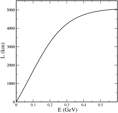
Recalling that the resonance energy is 120 MeV, we find that at this energy a baseline around 2000 km will yield maximal sensitivity to the terms linear in $\theta_{13}^{m}$. At twice the resonant energy, the necessary baseline has increased to 3700 km. Finally, the maximal baseline permitted by our constant density approximation is 4000 km, which corresponds to a neutrino energy of 270 MeV.

Regarding the larger mass-squared difference $\Delta_{31}$, the modification of this quantity needed to account for matter was the subtraction of $2E\lambda_{-}$. This term is at most on the order of $10^{-4}$ eV²; therefore, our assumptions regarding the incoherence of these oscillations is unaffected. In short, we may still take

$$\langle\sin^{2}\varphi_{31}^{m}\rangle=\frac{1}{2}.$$ (33)

With respect to the mixing angles, the mixing angle $\theta_{12}$ undergoes the greatest degree of modification to accommodate matter effects. This discussion is given in the next section. The effect upon $\theta_{13}$ is quite small. Estimating the maximum value of the additive correction, we have

$$\theta\simeq\frac{2EV}{\Delta_{31}}\theta_{13}\lesssim 0.09~{}\theta_{13}.$$ (34)

This represents at most ten percent correction for neutrinos of energies around 1 GeV. Should we only consider neutrino energies below 300 MeV, the correction becomes less than three percent. We shall consider this correction in our numerical analysis but drop the term in the analytical discussion. Incidentally, this correction to $\theta_{13}$ is the only place where the sign of $\Delta_{31}$ has any effect. Hence, we see that the hierarchy ambiguity plays a very small role in these calculations. Finally, the remaining mixing angle $\theta_{23}$ is insensitive to matter effects.

The upshot is that Eqs. (4)–(6) are still valid for neutrinos traveling through a constant density medium provided we make the appropriate substitutions for the mixing angles and small mass-squared difference. Neglecting the small correction $\theta$, the first order expansion of these probabilities about $\theta_{13}$ and $\varepsilon$ have not changed in form

$$\mathcal{P}_{e\mu}^{m}\simeq\sin^{2}{2\theta_{12}^{m}}\left[\frac{1}{2}-\varepsilon+\cot({2\theta_{12}^{m}})\theta_{13}\right]\sin^{2}\varphi_{21}^{m}\,,$$ (35)

and for $\nu_{\mu}$–$\nu_{\mu}$ oscillations, the probability becomes

$$\mathcal{P}_{\mu\mu}^{m}\simeq\frac{1}{2}-\sin^{2}{2\theta_{12}^{m}}\left[\frac{1}{4}-\varepsilon+\cot({2\theta_{12}^{m}})\theta_{13}\right]\sin^{2}\varphi_{21}^{m}.$$ (36)

IV Discussion

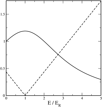
Aside from the adjustment in the ideal baseline, the change in the $\theta_{12}^{m}$ mixing angle is the most critical modification needed to account for matter effects. In the approximate formulae in Eqs. (35) and (36), the oscillatory terms are modulated by $\sin^{2}2\theta_{12}^{m}$ thereby affecting the amplitude of oscillations. Recalling Eq. (29), we note that, relative to vacuum oscillations, this factor enhances the oscillations in matter provided that the neutrino energy is less than twice the resonant energy. The new matter mixing angle is maximal whenever $E\simeq E_{R}$ and equal to the vacuum value whenever $E\ll E_{R}$ or $E\simeq 2E_{R}$. For neutrino energies greater than twice the resonant energy, the factor $\sin^{2}2\theta_{12}^{m}$ decreases significantly, effectively suppressing the amplitude of oscillations. In Fig. (2), we plot the ratio $\sin^{2}2\theta_{12}^{m}/\sin^{2}2\theta_{12}$ as a function of neutrino energy in order to demonstrate the enhancement and suppression of the oscillation amplitude relative to vacuum oscillations. At an energy of 270 MeV, which is $2.25E_{R}$, we find that the amplitude will be suppressed by a factor of 0.9 relative to vacuum oscillations.

Figure 2: The solid line is the ratio $\sin^{2}2\theta_{12}^{m}/\sin^{2}2\theta_{12}$. The dotted line is the curve $\cot 2\theta_{12}^{m}$. We have set $\theta_{12}=0.58$ and plot the curves as functions of the dimensionless ratio $E/E_{R}$.

Another notable feature of the first order expansions of the oscillation channels in Eqs. (35) and (36) are the terms which appear within the square brackets. Given the lack on knowledge in the true values of $\theta_{23}$ and $\theta_{13}$, it is apparent from the equations that a measurement at these baselines of, say, the $\nu_{e}$–$\nu_{\mu}$ probability does not directly resolve the values of these mixing angles. Indeed, we see that a host of parameters can satisfy a measurement provided the linear relation

$$\varepsilon-\cot({2\theta_{12}^{m}})\theta_{13}=\mathrm{const}$$ (37)

holds.

As the slope of this relation, $\cot{2\theta_{12}^{m}}$, varies with neutrino energy, its value is represented by the dotted curve in Fig. (2). For energies greater than the $E_{R}$, the slope increases linearly with neutrino energy. Of particular importance are two points. First, at the resonance energy we see that both oscillation channels do not depend linearly on $\theta_{13}$; a measurement of such neutrinos could at best improve the bounds upon $\theta_{23}$ while potentially resolving the octant of $\theta_{23}$. As our constant density approximation is really only valid up to 270 MeV, we note from the graph the value of $\cot 2\theta_{12}^{m}$ is 0.54 at this energy. A measurement at this energy would have implications for both the sign of $\theta_{13}$ and the octant of $\theta_{23}$.

The aim of this paper is to determine how a measurement at this baseline of either the $\nu_{e}$–$\nu_{\mu}$ or $\nu_{\mu}$–$\nu_{\mu}$ oscillation channel will affect the values of $\theta_{23}$ and $\theta_{13}$. To most explicitly demonstrate this, we will create some mock experimental data and combine it with the present knowledge of these mixing angles. To this end, we introduce a $\chi^{2}$ function made up of three parts

$$\chi^{2}=\chi^{2}_{13}+\chi^{2}_{23}+\chi^{2}_{\mathcal{P}}.$$ (38)

For the first term, we include information from CHOOZ via the simple relation

$$\chi^{2}_{13}=\frac{(\theta_{13}-\theta_{13}^{0})^{2}}{\sigma_{13}^{2}}$$ (39)

where the best fit value is $\theta_{13}^{0}=0$ and the standard deviation is $\sigma_{13}=0.15$. Similarly, we include information on $\theta_{23}$ in the same manner where the best fit value is maximal $\theta_{23}^{0}=0.785$ and the standard deviation is $\sigma_{23}=0.07$.

The final term in $\chi^{2}$ represents our mock data. For concreteness, we choose the electron-muon oscillation channel. As with the others, we define $\chi^{2}_{\mathcal{P}}$ with respect to a best fit $\mathcal{P}_{e\mu}^{0}$ and a standard deviation which we take to be ten percent of the best fit

$$\chi^{2}_{\mathcal{P}}=\frac{(\mathcal{P}_{e\mu}(\theta_{13},\theta_{23})-\mathcal{P}_{e\mu}^{0})^{2}}{\sigma_{\mathcal{P}}^{2}}$$ (40)

We assume, as well, a mono-energetic source of 270 MeV measured at the ideal baseline of 4000 km. The question remains as to what value we assign our measured best fit. At present, the only experimentally observed neutrinos of this energy and baseline occur in the sub-GeV sample of the Super-K atmospheric experiment superk . A detailed analysis of the oscillation channels of interest has been performed in Ref. smirnov1 . Our first order approximations in $\varepsilon$ and $\theta_{13}$ exhibit some of the significant behavior given in this reference. Briefly, assuming neutrino oscillations and CP invariance, one would expect the detector-to-source ratio of atmospheric electron-like neutrinos to be

$$\mathcal{R}_{e}=\mathcal{P}_{ee}+r\mathcal{P}_{e\mu},$$ (41)

where $r$ is the ratio of muon to electron neutrinos in the upper atmosphere. For energies of a few hundred MeV, one has $r\simeq 2$. For those which traverse the mantle only with baselines over $3\times 10^{3}$ km, we may use the expression from Eq. (35) along with a first order expansion of $\mathcal{P}_{ee}$ to determine the approximate expectation ratio

$$\mathcal{R}_{e}\simeq 1+2\sin^{2}2\theta_{12}^{m}\left[\cot({2\theta_{12}^{m}})\theta_{13}-\varepsilon\right]\sin^{2}\varphi_{21}^{m}.$$ (42)

In-depth analyses of Super-K smirnov1 ; eexcess ; ggth23 cite the oscillations discussed herein as a potential explanation for an excess of electron-like events in the sub-GeV sample. If this excess is indeed real, then our approximation indicates

$$\cot({2\theta_{12}^{m}})\theta_{13}-\varepsilon>0.$$ (43)

Though this expression is not the result of a detailed analysis of the experiment, its qualitative features should still be valid. With that said, the inequality in (43) indicates that the potential excess of electrons in the sub-GeV sample can be accounted for by a range of parameters. Should $\theta_{13}=0$ for instance, we find that $\varepsilon<0$ which indicates that $\theta_{23}$ is in the first octant. Alternatively, should 2–3 mixing be maximal, the above inequality indicates that $\theta_{13}$ is positive.

This qualitative understanding is confirmed in more detailed analyses of experiments which have very long baselines. In Ref. ggth23 , preliminary evidence indicates that $\theta_{23}$ lies in the first octant. Within this full three-neutrino analysis (labeled A), the best fit mixing angles are found to be

$$\theta_{12}^{A}=0.575,\qquad\theta_{13}^{A}=0.0,\qquad\theta_{23}^{A}=0.745,$$ (44)

which in the present context is expressed by $\varepsilon=-0.04$. Additionally, in Ref. ggpostks , a full three-neutrino analysis of the world’s data is performed. When 2–3 mixing is assumed maximal, the best fit mixing angles (labeled B) are determined to be

$$\theta_{12}^{B}=0.591,\qquad\theta_{13}^{B}=0.095,\qquad\theta_{23}^{B}=0.785.$$ (45)

These two parameter sets are consistent with the correlation between $\theta_{13}$ and $\varepsilon$ which we have indicated above. Employing the average of the two values for the solar mixing angle $\overline{\theta}_{12}=0.58$, we find

$$\frac{\theta_{23}^{B}-\theta_{23}^{A}}{\theta_{13}^{B}-\theta_{13}^{A}}=\cot 2\overline{\theta}_{12},$$ (46)

to four percent. Thus, although a small effect, the contribution to the $e$-like sub-GeV excess for atmospheric data smirnov1 introduces a correlation between the extracted values of $\theta_{13}$ and $\varepsilon$.

In Ref. ggth23 it is shown that future atmospheric data will further constrain the value of $\theta_{23}$ and perhaps determine its octant, this for $\theta_{13}=0$. We have here implicitly generalized this result. Future atmospheric data will provide information on the value of the function $\cot(2\theta_{12}^{m})\,\theta_{13}-\varepsilon$ in addition to the cleaner measurements of $\varepsilon$.

Though these values are not statistically robust, we may use them as an indication of where a best fit point might lie. For the best fit, we choose the average value for the solar mixing angle and the values for $\theta_{13}$ and $\theta_{23}$ from parameter set A in Eq. (44). We may now determine the acceptable regions for these two mixing angles given our mock data and the existing knowledge. From the $\chi^{2}$ function, we are able to plot the 68%, 90%, and 95% CL allowed regions in Fig. (3).

Figure 3: Given the mock data for the $\mathcal{P}_{e\mu}$ measurement at the ideal baseline for mono-energetic neutrinos of 270 MeV, we construct a hypothetical allowed region for $\theta_{13}$ and $\theta_{23}$. We draw the 68%, 90%, and 95% CL contours.

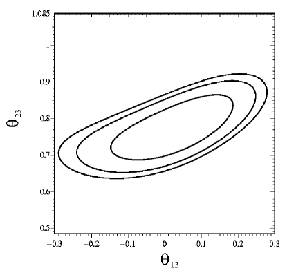
The best fit value is $\theta_{13}=0.04$ and $\theta_{23}=0.775$. The slope of the upper portion of the closed contours in the figure is given by $\cot{2\theta_{12}^{m}}$. We note that this mock data indicates a preference for positive $\theta_{13}$ and first-octant $\theta_{23}$; however, the possibility remains that they lie elsewhere.

V Conclusion

We have expanded the oscillation probabilities $\mathcal{P}_{e\mu}$ and $\mathcal{P}_{\mu\mu}$ to first order in $\theta_{13}$ and $\varepsilon$, where $\varepsilon$ indicates the deviation of the mixing angle $\theta_{23}$ from maximal. This was done for neutrinos propagating in the vacuum and in a constant density mantle. For the oscillations in matter, it was shown that the amplitude of the oscillations is enhanced relative to vacuum for neutrino energies less than twice the resonant energy; the amplitude was suppressed at energies greater than this mark. Terms linear in $\theta_{13}$ were of significance whenever the matter-modified solar mass-squared difference $\Delta_{21}^{m}$ was in the oscillatory region. The ideal baseline, defined by the first peak or trough of these oscillations, was determined as a function of neutrino energy. For a maximum baseline of 4000 km, this energy was found to be 270 MeV. At this energy and ideal baseline, the relation between the deviation of $\theta_{23}$ from maximal mixing and $\theta_{13}$ was examined by creating mock data. The mock data demonstrated what was found in the approximate equations; that is, $\theta_{13}$ and $\varepsilon$ are linearly related via a slope of $\cot{2\theta_{12}^{m}}$. The energy dependence of this slope was elucidated. For an energy of 270 MeV, it was shown to be 0.54; this factor increases linearly with neutrino energy, assuming the energy is greater than the resonant energy.

It is seen from the mock data that this ideal measurement could help determine the algebraic sign of $\theta_{13}$ and perhaps the octant of $\theta_{23}$. For a measurement most sensitive to the octant of $\theta_{23}$, one would like the neutrino energy to be near the MSW resonance of 120 MeV. At this point, the slope is minimal because $\cot{2\theta_{12}^{m}}=0$. To best determine the sign of $\theta_{13}$, one would like the slope relating the mixing angle and $\varepsilon$ to be as large as possible without completely suppressing the oscillation amplitude. To achieve this, one would require higher energy neutrinos and, therefore, longer baselines. Our constant density treatment would no longer be valid as these neutrinos would certainly traverse the core of the earth and parametric resonances would be of consequence. We leave a detailed analysis of this case to future work.