Time–Reversal–Violating Schiff Moment of ${}^{199}{\rm Hg}$

Abstract

We calculate the Schiff moment of the nucleus ${}^{199}{\rm Hg}$, created by $\pi$NN vertices that are odd under parity (P) and time–reversal (T). Our approach, formulated in diagrammatic perturbation theory with important core–polarization diagrams summed to all orders, gives a close approximation to the expectation value of the Schiff operator in the odd–A Hartree–Fock–Bogoliubov ground state generated by a Skyrme interaction and a weak P– and T–odd pion–exchange potential. To assess the uncertainty in the results, we carry out the calculation with several Skyrme interactions, the quality of which we test by checking predictions for the isoscalar–E1 strength distribution in ${}^{208}{\rm Pb}$, and estimate most of the important diagrams we omit.

I Introduction

The existence of a permanent electric dipole moment (EDM) in leptons, neutrons or neutral atoms is direct evidence for time–reversal (T) violation. Because of the CPT theorem, the search for EDMs can provide us valuable information about sources of CP violation. Though a phase in the Cabibbo–Kobayashi–Maskawa matrix is enough to account the level of CP violation in kaon and B–meson decays, it cannot explain the observed matter/anti–matter asymmetry in the Universe. Physics that can (and new physics at the weak scale more generically) should produce EDMs not far from current upper limits.

So far no EDMs have been observed, but experiments are continually improving. Here we are interested in the conclusions that can be drawn from the measured upper limit Romalis et al. (2001) in ${}^{199}{\rm Hg}$, a diamagnetic atom. The largest part of its EDM most likely comes from T violation in the nucleus, caused by a T–violating (and parity–violating) component of the nucleon–nucleon interaction. The atomic EDM is generated by the subsequent interaction of the nucleus with the electrons.

That interaction is more subtle than one might think. If the nucleus and electrons were non–relativistic point–particles interacting solely via electrostatic forces, the electrons would rearrange in response to a nuclear EDM to cancel it essentially exactly. Fortunately, as was shown by Schiff Schiff (1963), the finite size of the nucleus leads to a residual atomic EDM. It turns out, however, that the relevant nuclear quantity is not the nuclear EDM but rather the nuclear “Schiff moment”

$$S~{}\equiv~{}\langle\Psi_{0}|S^{z}|\Psi_{0}\rangle~{},$$ (1)

which is the nuclear ground–state expectation value, in the substate $|\Psi_{0}\rangle$ with angular momentum projection $M_{J}$ equal to the angular momentum $J$, of the $z$–component of the “Schiff operator”

$$\bm{S}~{}=~{}\frac{e}{10}\,\sum_{p=1}^{Z}\left(r^{2}_{p}-\frac{5}{3}\,\langle{r}^{2}\rangle_{\rm ch}\right)\bm{r}_{p}~{}.$$ (2)

Here $e$ is the charge of the proton, $\langle r^{2}\rangle_{\rm ch}$ is the mean squared radius of the nuclear charge distribution, and the sum is restricted to protons.

For the Schiff moment to exist, P and T must be violated by the nuclear Hamiltonian. We assume that whatever its ultimate source, the T violation works its way into a meson–mediated P– and T–violating NN interaction generated from a Feynman graph containing a meson propagator, the usual strong meson–NN strong vertex and a (much weaker) P– and T–violating meson–NN vertex. The second vertex can take three different forms in isospin space. References Herczeg (1988); Griffiths and Vogel (1991); Towner and Hayes (1994) showed that short–range nuclear correlations and a fortuitous sign make the contribution of $\rho$– and $\omega$–exchange to the interaction small compared to that of pion–exchange if the T–violating coupling constants of the different mesons are all about the same, and so we neglect everything but pion exchange. The most general P– and T–odd NN potential then has the form ($\hbar=c=1$)

$$W(\bm{r}_{a}-\bm{r}_{b}) = -\frac{{\rm g}m_{\pi}^{2}}{8\pi m_{\rm N}}\left\{\left[{\rm\bar{g}}_{0}\left(\bm{\tau}_{a}\cdot\bm{\tau}_{b}\right)-\frac{{\rm\bar{g}}_{1}}{2}\left(\tau_{a}^{z}+\tau_{b}^{z}\right)+{\rm\bar{g}}_{2}\left(3\tau_{a}^{z}\tau_{b}^{z}-\bm{\tau}_{a}\cdot\bm{\tau}_{b}\right)\right]\left(\bm{\sigma}_{a}-\bm{\sigma}_{b}\right)-\right.$$ (3)

$$\mbox{}\left.-\frac{{\rm\bar{g}}_{1}}{2}\left(\tau_{a}^{z}-\tau_{b}^{z}\right)\left(\bm{\sigma}_{a}+\bm{\sigma}_{b}\right)\right\}\cdot\left(\bm{r}_{a}-\bm{r}_{b}\right)\frac{{\rm exp}\left(-m_{\pi}|\bm{r}_{a}-\bm{r}_{b}|\right)}{m_{\pi}|\bm{r}_{a}-\bm{r}_{b}|^{2}}\left[1+\frac{1}{m_{\pi}|\bm{r}_{a}-\bm{r}_{b}|}\right]~{},$$

where $m_{\pi}$ is the mass of the pion, $m_{\rm N}$ that of the nucleon, $\tau^{z}|p\rangle=-|p\rangle$, ${\rm g}\equiv 13.5$ is the strong $\pi$NN coupling constant, and the $\bar{\rm g}_{i}$ are the isoscalar ($i=0$), isovector ($i=1$), and isotensor ($i=2$) PT–odd $\pi$NN coupling constants. A word of caution here: more than one sign convention for the $\bar{\rm g}$’s is in use. Our $\bar{\rm g}_{0}$ and $\bar{\rm g}_{1}$ are defined with a sign opposite to those used by Flambaum et. al Flambaum et al. (1986); Flambaum and Ginges (2002) and by Dmitriev et. al Dmitriev and Sen’kov (2003); Dmitriev et al. (2005).

The goal of this paper is to calculate the dependence of the Schiff moment of ${}^{199}{\rm Hg}$ on the T–violating $\pi$NN couplings (we leave the dependence of these couplings on fundamental sources of CP violation to others) so that models of new physics can be quantitatively constrained. An accurate calculation is not easy because the Schiff moment depends on the interplay of the Schiff operator with complicated spin– and space–dependent correlations induced by the the two–body interaction $W$. In the early calculation by Flambaum, Khriplovich and Sushkov almost two decades ago Flambaum et al. (1986), the correlations were taken to be admixtures of simple 1–particle 1–hole excitations into a Slater determinant produced by a one–body Wood–Saxon potential.

More recent work Dmitriev and Sen’kov (2003); Dmitriev et al. (2005) made significant improvements by treating the correlations in the RPA after generating an approximately self–consistent one–body potential. However, that work used only the relatively schematic Landau–Migdal interaction (in addition to $W$) in the RPA and mean–field equations, and did not treat pairing self consistently. The reliance on a single strong interaction makes it difficult to analyze uncertainty. Such an analysis seems to be particularly important in ${}^{199}{\rm Hg}$, the system with the best experimental limit on its EDM. The calculated Schiff moment of Refs. Dmitriev and Sen’kov (2003); Dmitriev et al. (2005) in that nucleus depends extremely weakly on the isoscalar coefficient ${\rm\bar{g}}_{0}$, a result of coincidentally precise cancellations among single–particle and collective excitations. They might be less precise when other interactions are used.

Here we make several further improvements. Our mean field, which we calculate in ¹⁹⁸Hg before treating core polarization by the valence nucleon, includes pairing and is exactly self consistent. Pairing changes the RPA to the quasiparticle–RPA (QRPA), a continuum version of which we use to obtain ground–state correlations. Most importantly, we carry out the calculation with several sophisticated (though still phenomenological) Skyrme NN interactions, the appropriateness of which we explore by examining their ability to reproduce measured isoscalar–E1 strength (generated by the isoscalar component of the Schiff operator) in ²⁰⁸Pb. The use and calibration of more than one such force allows us to get a handle on the uncertainty in our final results.

The rest of this paper is organized as follows: Section II describes our approach and the Skyrme interactions we use, and includes their predictions for strength distributions that bear on the Schiff moment. Section III presents our results and an analysis of their uncertainty, including a calculation in the simpler nucleus ²⁰⁹Pb that allows us to check the size of effects we omit in ${}^{199}{\rm Hg}$. Section IV is a conclusion.

II Procedure for evaluating Schiff moments

II.1 Method

Our Schiff moment is a close approximation to the expectation value of the Schiff operator in the completely self–consistent one–quasiparticle ground state of ${}^{199}{\rm Hg}$, constructed from a two–body interaction that includes both a Skyrme potential and the P– and T–violating potential $W$. It is an approximation because we do not treat $W$ in a completely self consistent way, causing an error that we estimate to be small in the Section III. In addition, we do not actually carry out the mean–field calculation in ${}^{199}{\rm Hg}$ itself. Instead, we start from the HF+BCS ground–state of the even–even nucleus ${}^{198}{\rm Hg}$ and add a neutron in the $2p_{1/2}$ level. We then treat the core–polarizing effects of this neutron in the QRPA. A self–consistent core with QRPA core polarization is completely equivalent to a fully self–consistent odd–A calculation Brown (1970). We omit one part of the QRPA core polarization, again with an estimate showing its contribution to be insignificant.

A good way to keep track of the two interactions and their effects is to formulate the calculation (and corrections to it) as a sum of Goldstone–like diagrams, following the shell–model effective–operator formalism presented, e.g., in Ref. Ellis and Osnes (1997). The one difference between our diagrams and he usual “Brandow” kind is that our fermion lines will represent BCS quasiparticles rather than pure particles or holes. Our diagrams reduce to the familiar kind in the absence of pairing.

We begin, following a spherical HF+BCS calculation in ${}^{198}{\rm Hg}$ (in a 20–fm box with mixed volume and surface pairing fixed as in Ref. Bender et al. (2002)), by dividing the Hamiltonian into unperturbed and residual parts. The unperturbed part, expressed in the quasiparticle basis, is

$$H_{0}=T+V_{00}+V_{11}~{},$$ (4)

where $T$ is the kinetic energy and $V$ the Skyrme interaction, with subscripts that refer to the numbers of quasiparticles the operator creates and destroys. The residual piece is

$$H_{\rm res}=W+V_{22}+V_{13}+V_{31}+V_{04}+V_{40}~{}.$$ (5)

The interaction $W$ can also be expanded in terms of quasiparticle creation and annihilation operators; all the terms are included in $H_{\rm res}$, though $W_{00}$ vanishes because $W$ is a pseudoscalar operator. The valence “model space” of effective–operator theory is one–dimensional: a quasiparticle with $u=0$ and $v=1$ (i.e. a particle, since it is not part of a pair) in the the $a\equiv(2p_{1/2},m=1/2)$ level. The unperturbed ground state $|\Phi_{a}\rangle$ is simply this one–quasiparticle state. Then the expectation value of $S^{z}$, Eq. (1), in the full correlated ground state $|\Psi_{a}\rangle\equiv|\Psi_{0}\rangle$ is given by

$$\langle\Psi_{a}|S^{z}|\Psi_{a}\rangle~{}=~{}{\cal N}^{-1}\langle\Phi_{a}|\left[1+H_{\rm res}\left(\frac{Q}{\epsilon_{a}-H_{0}}\right)+\cdots\right]S^{z}\left[1+\left(\frac{Q}{\epsilon_{a}-H_{0}}\right)H_{\rm res}+\cdots\right]|\Phi_{a}\rangle~{}.$$ (6)

Here $\epsilon_{a}$ is the single–quasiparticle energy of the valence nucleon, the operator $Q$ projects onto all other single–quasiparticle states, ${\cal N}$ is a normalization factor that, we will argue later, is very close to one, and the dots represent higher–order terms in $H_{\rm res}$. To evaluate the expression, we write $S^{z}$ in the quasiparticle basis as $S^{z}=S_{11}+S_{02}+S_{20}$ ($S_{00}$ vanishes for the same reason as $W_{00}$).

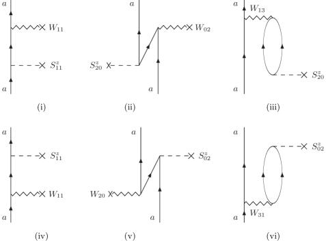
Figure 1: First–order quasiparticle diagrams contributing to the Schiff moment. Diagrams (i), (ii), (iv) and (v) do not contribute if the valence nucleon is a neutron, which is the case in ${}^{199}{\rm Hg}$. Diagram (vi) is the complex conjugate of diagram (iii).

The zeroth–order contribution to the Schiff moment in Eq. (6) vanishes because the Schiff operator cannot connect two states with the same parity, and also because the Schiff operator acts only on protons while the valence particle in ${}^{199}{\rm Hg}$ is a neutron. (There are no center–of–mass corrections to the effective charges Sushkov et al. (1984).) The terms that are first order in $H_{\rm res}$ do not include the strong interaction $V$ because it has a different parity from the Schiff operator. Thus the lowest order contribution to the Schiff moment is

$$\langle\Psi_{a}|S^{z}|\Psi_{a}\rangle^{\rm first-order}~{}=~{}\langle-|q_{a}\left[W\left(\frac{Q}{\epsilon_{a}-H_{0}}\right)S^{z}\right]q^{{\dagger}}_{a}|-\rangle+{\rm c.c.}~{},$$ (7)

where $q^{{\dagger}}_{a}$ is the creation operator for a quasiparticle in the valence level ${a}$ and $|-\rangle$ is the no–quasiparticle BCS vacuum describing the even–even core, so that $|\Phi_{a}\rangle$ is just $q^{{\dagger}}_{a}|-\rangle$. The contribution of Eq. (7) in an arbitrary nucleus can be represented as the sum of the diagrams in Fig. 1, the rules for which we give in the Appendix. In ${}^{199}{\rm Hg}$, because the valence particle is a neutron, only diagrams (iii) and (vi) are nonzero. We can interpret diagram (iii) as the Schiff operator exciting the core to create a virtual three–quasiparticle state, which is then de–excited back to the ground state when the valence neutron interacts with the core through $W$. This diagram and its partner (vi) are what was evaluated by Flambaum et al. Flambaum et al. (1986), though their mean field was a simple Wood–Saxon potential, their $W$ was a zero–range approximation that didn’t include exchange terms, and they neglected pairing.

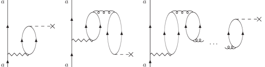
Figure 2: Examples of diagrams contributing to the collective response to the Schiff operator. The sum of all these diagrams is represented in Fig. 3(i). The broken line represents the action of the Schiff operator (as in Fig. 1), the zig-zag line represents the P– and T–violating interaction (also as in Fig. 1), and the looped line represents a generic Skyrme interaction.

Core polarization, implemented through a version of the canonical–basis QRPA code reported in Ref. Terasaki et al. (2005) (with residual spurious center–of–mass motion removed following Ref. Agrawal et al. (2003)), can be represented by a subset of the higher–order diagrams. Because $W$ is so weak, we need only include it in first order. The higher order terms in $V$ that we include have the effect of replacing the two–quasiparticle bubble in (iii) and (vi) of Fig. 1 with chains of such bubbles (see Fig. 2), as well adding diagrams in which the QRPA bubble chains are excited through a strong interaction of the core with the valence neutron. We therefore end up evaluating diagrams labeled A, B1, and B2, in Fig. 3 (plus two more of type B in which the interaction $W$ is below the Schiff operator). The explicit expression for diagram A, the first on the left in the figure, is

$$\langle\Psi_{a}|S^{z}|\Psi_{a}\rangle_{\rm diag-A}~{}=~{}-\sum_{\lambda}\sum_{{k}>{l}}\sum_{k^{\prime}>l^{\prime}}Z^{\lambda\ast}_{{k}{l}}\langle-|S^{z}_{02}|{k}{l}\rangle Z^{\lambda}_{k^{\prime}l^{\prime}}\langle{a}k^{\prime}l^{\prime}|W_{31}|{a}\rangle{\cal E}_{\lambda}^{-1}~{}.$$ (8)

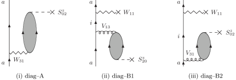
Figure 3: QRPA diagrams contributing to the Schiff moment. The filled bubble represents an infinite sum of quasiparticle bubbles, including all the forward and backward amplitudes. The two B diagrams have partners (not shown) in which $W$ acts below $S^{z}$.

Here, $Z^{\lambda}_{{k}{l}}\equiv X^{\lambda}_{{k}{l}}+Y^{\lambda}_{{k}{l}}$ represents the QRPA amplitudes (the sum appears because the matrix elements of all our operators are real) and ${\cal E}_{\lambda}$ is the energy of the collective state $\lambda$ in ${}^{198}{\rm Hg}$. The quasiparticle matrix elements $\langle-|S^{z}_{02}|{k}{l}\rangle$ and $\langle{a}{k}{l}|W_{31}|{a}\rangle$ are related to the usual particle matrix elements $\langle{k}|S^{z}|{l}\rangle$ and $\langle{a}{k}|W|{a}{l}\rangle$ through the transformations discussed in the Appendix. In the absence of QRPA correlations, the $X$ and $Y$ amplitudes are 1 or 0, and Eq. (8) reduces to that associated with diagrams (iii) and (vi) of Fig. 1.

Diagrams B1 and B2 of Fig. 3 have the explicit expressions

$$\langle\Psi_{a}|S^{z}|\Psi_{a}\rangle_{\rm diag-B1} = -2\sum_{\lambda}\sum_{i}\sum_{{k}>{l}}\sum_{k^{\prime}>l^{\prime}}\langle{a}|W_{11}|{i}\rangle Z^{\lambda\ast}_{{k}{l}}\langle{i}|V_{13}|{a}{k}{l}\rangle Z^{\lambda}_{k{\prime}l^{\prime}}\langle k^{\prime}l^{\prime}|S^{z}_{20}|-\rangle(\epsilon_{a}-\epsilon_{i})^{-1}{\cal E}_{\lambda}^{-1}~{},$$ (9)

$$\langle\Psi_{a}|S^{z}|\Psi_{a}\rangle_{\rm diag-B2} = -2\sum_{\lambda}\sum_{i}\sum_{{k}>{l}}\sum_{k^{\prime}>l^{\prime}}\langle{a}|W_{11}|{i}\rangle Z^{\lambda\ast}_{{k}{l}}\langle-|S^{z}_{02}|{k}{l}\rangle Z^{\lambda}_{k^{\prime}l^{\prime}}\langle{i}k^{\prime}l^{\prime}|V_{31}|{a}\rangle(\epsilon_{a}-\epsilon_{i})^{-1}({\cal E}_{\lambda}-\epsilon_{a}+\epsilon_{i})^{-1}~{}.$$ (10)

The factor 2 accounts for diagrams not shown in Fig. 3 in which $W$ acts below the QRPA bubble, and the $\epsilon$’s are quasiparticle energies. The difference between Eq. (9) and Eq. (10) is mainly in the three-quasiparticle intermediate states.

A complete QRPA calculation that is first order in $W$ would also include versions of diagram A in which $W$ trades places with one of the $V$’s in the bubble sum. We don’t evaluate such diagrams but estimate their size (which we find to be small) rom calculations in the simpler nucleus ${}^{209}{\rm Pb}$ in the next section. We also use that nucleus to examine other low–order diagrams not included in the bubble sum of diagram A.

Why do we expect the QRPA subset of diagrams to be sufficient? The reason is that they generally account for the collectivity of virtual excitations in a reliable way when calculated with Skyrme interactions. We illustrate this statement below with some calculations of isoscalar–E1 strength in ${}^{208}{\rm Pb}$.

II.2 Interactions

We carry out the calculation with 5 different Skyrme interactions: our preferred interaction SkO^′ Bender et al. (2002); Reinhard et al. (1999) (preferred for reasons discussed in Ref. Engel et al. (2003)), and the older, commonly used interactions SIII Beiner et al. (1975), SkM^∗ Bartel et al. (1982), SLy4 Chabanat et al. (1998), and SkP Dobaczewski et al. (1984). To get some idea of how well they will work, we calculate the strength distribution of the isoscalar–E1 operator

$$\bm{D}_{0}~{}=\sum_{p=1}^{Z}r_{p}^{2}\bm{r}_{p}+\sum_{n=1}^{N}r_{n}^{2}\bm{r}_{n}~{}.$$ (11)

This operator is interesting because it is the isoscalar version of the Schiff operator (the isoscalar version of the second term in the Schiff operator acts only on the center of mass and so doesn’t appear in $\bm{D}_{0}$). The isoscalar–E1 strength, measured, e.g., in ${}^{208}{\rm Pb}$ Clark et al. (2001), seems to fall mainly into two peaks. The high–energy peak, related to the compressibility coefficient ${\rm K}_{\infty}$, Davis et al. (1997); Hamamoto et al. (1998); Colò et al. (2000); Vretenar et al. (2000); Clark et al. (2001); Abrosimov et al. (2002); Shlomo and Sanzhur (2002), is observed to lie between 19 and 23 MeV, depending on the experimental method used Davis et al. (1997); Clark et al. (2001). Recent interest has focused on a smaller but still substantial low–energy peak around $12~{}{\rm MeV}$, which has been studied theoretically in the RPA Colò et al. (2000); Vretenar et al. (2000) as well as experimentally Clark et al. (2001).

Figure 4 shows the predictions of several Skyrme interactions in the RPA, with widths of 1 MeV introduced by hand following Ref. Hamamoto et al. (1998), for the isoscalar–E1 strength distribution in ${}^{208}{\rm Pb}$. The figure also shows the locations of the measured low– and high–energy peaks of Davis et al. Davis et al. (1997) and of Clark et al. Clark et al. (2001). Nearly all self–consistent RPA calculations, including ours (except with SkP) over–predict the energy of the larger peak by a few MeV Colò et al. (2000); Clark et al. (2001). SIII does a particularly poor job. The predicted low–energy strength is closer to experiment, though usually a little too low. Table 1 summarizes the situation. Unfortunately, the data are not precise enough to extract much more than the centroids of the two peaks. Since the Schiff–strength distribution in ${}^{199}{\rm Hg}$ helps determine the Schiff moment, it would clearly be useful to have better data, either in that nucleus or a nearby one such as ${}^{208}{\rm Pb}$.

The isovector–E1 strength distribution also bears on the Schiff moment through the second term of the Schiff operator, but it is well understood experimentally and generally reproduced fairly well by Skyrme interactions.

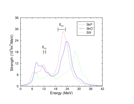
Figure 4: Isoscalar–E1 strength distributions for ${}^{208}{\rm Pb}$ predicted by the Skyrme interactions SkP, SkO^′ and SIII in self–consistent HF+RPA. The experimental bounds on the low–energy ($\rm{E_{x1}}$) and high–energy (${\rm E_{x2}}$) peaks are also shown (see Table 1).

		low (MeV)	high (MeV)
SkM⋆		$11.0$	$25.3$
SkP		$10.0$	$23.4$
SIII		$11.6$	$28.3$
SLy4		$11.4$	$26.4$
SkO′		$10.3$	$24.8$
Experiment Davis et al. (1997)		$-$	$22.4\pm 0.5$
Experiment Clark et al. (2001)		$12.2\pm 0.6$	$19.9\pm 0.8$

Table 1: Comparison between experimental and theoretical results for the centroids of the low- and high-energy peaks in the distribution of isoscalar E1 strength in ${}^{209}{\rm Pb}$. The experimental results are from Refs. Clark et al. (2001) and Davis et al. (1997). (Ref. Davis et al. (1997) identifies only the high-energy peak.) The theoretical distributions are from self-consistent HF+RPA calculations with five different Skyrme interactions.

III Results and estimate of uncertainty

III.1 Results with several forces

The Schiff moment can be written as

$$S=a_{0}~{}{\rm g\bar{g}}_{0}+a_{1}~{}{\rm g\bar{g}}_{1}+a_{2}~{}{\rm g\bar{g}}_{2}~{},$$ (12)

where ${\rm\bar{g}}_{i}$ are the P– and T–odd $\pi$NN coupling constants and all the nuclear physics is summarized by the three coefficients $a_{i}$. We present our results for these coefficients by showing the effects, in turn, of several improvements on early calculations.

The first calculations of Schiff moments Flambaum et al. (1986), as noted above, correspond to our first–order diagrams (iii) and (vi) of Fig. 1 but with no pairing, with a simple Wood–Saxon potential in place of a self–consistent mean field, and with the zero–range limit of the direct part of $W$. The results of Ref. Flambaum et al. (1986) are given here in the first line of Tab. 2.

	$a_{0}$	$a_{1}$	$a_{2}$
Ref. Flambaum et al. (1986)	$0.087$	$0.087$	$0.174$
Naive limit	$0.095$	$0.095$	$0.190$
Diagram A only	$0.018$	$0.034$	$0.031$
Full result	$0.010$	$0.074$	$0.018$

Table 2: Calculated coefficients $a_{i}$ from Ref. Flambaum et al. (1986) and with the Skyrme interaction SkO^′ in several limits (see text). The full result is in the last line.

When we repeat the calculation, evaluating diagrams (iii) and (vi) with $W$ approximated by its direct part in the zero–range limit and with the mean field from the Skyrme interaction SkO^′ (so that the only differences in the calculations are the one–body potential and BCS paring), we get the coefficients in second line of the table.

The finite range of the potential reduces the $a_{i}$ from these zero–range values by 30–40%, depending on the Skyrme interaction used. Exchange terms, when the range is finite, decrease $a_{0}$ by a few percent, have no effect on $a_{1}$ and increase $a_{2}$ by half the amount they decrease $a_{0}$.

The three coefficients in lines 1 and 2 of the table are not independent; the isotensor coefficient is exactly two times larger than the isovector and isoscalar coefficients. Because the valence neutron must excite core protons to couple to the Schiff operator through (iii) and (vi) of Fig. 1, only the neutron–proton part of $W$ contributes, and under the assumptions of no core spin, no exchange terms, and zero–range, $W$ reduces to

$$W^{\rm contact}_{\rm direct}(\bm{r}_{n}-\bm{r}_{p})~{}=~{}-\frac{1}{2m_{\pi}^{2}m_{\rm N}}({\rm g}{\rm\bar{g}}_{0}+{\rm g}{\rm\bar{g}}_{1}+2{\rm g}{\rm\bar{g}}_{2})\bm{\sigma}_{n}\cdot\bm{\nabla}_{n}\delta(\bm{r}_{n}-\bm{r}_{p})~{},\qquad{\rm no~{}core~{}spin}$$ (13)

Thus, in the approach of Flambaum et al. Flambaum et al. (1986), the Schiff moment is a function of a single parameter, usually called $\eta_{np}$. Exchange terms add another independent parameter and QRPA bubbles bring in a third. This last term arises because the valence neutron, besides exciting a proton quasiparticle pair in the core, can now excite neutron quasiparticle pairs that annihilate and create proton pairs inside the bubble that then couple to the Schiff operator (see Fig. 2). Thus, in our complete calculation, particularly when the B diagrams are included, the three coefficients $a_{i}$ are independent.

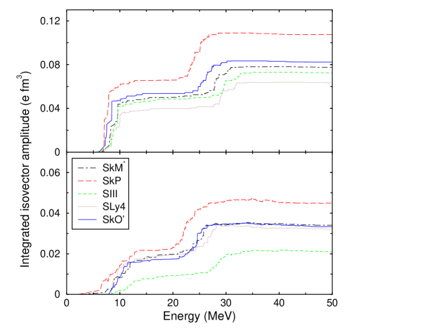
Figure 5: Integrated contribution of ${\rm\bar{g}}_{1}$ to diagram A as a function of core–excitation energy (the value of the isovector part of the diagram is given by the lines at large energy) in the two–quasiparticle limit (top) and in the QRPA (bottom) for five different Skyrme interactions. The two bumps are at the energies of the low– and high–lying peaks of the isoscalar–E1 strength distribution.

The collectivity of the core turns out to be very important. As can be seen in the third line of Tab. 2, when the single–particle bubble in the calculation above is replaced by the full QRPA bubble sum to give diagram A, all three $a_{i}$ shrink substantially. The reason is that the Schiff strength is pushed on average to higher energies, both in the low–lying and high–lying analogs of the isoscalar–E1 distribution. (The high–lying peak actually is replaced by two peaks, the higher of which is at about 38 MeV. There is no peak corresponding to the giant isovector–E1 resonance, as was shown in Ref. Engel et al. (1999).) The reduction is greater in the isoscalar and tensor channels — a factor of 4 to 6 depending on the Skyrme interaction — than in the isovector channel, where it is a factor of 2 to 3. Figure 5 shows the integral of the contribution to diagram A as a function of core–excitation energy (so that at large energy the lines approach the value for the diagram) for $a_{1}$, with and without the bubble sum, for all 5 forces.

The reason for the difference in the size of the reduction is that the ${\rm\bar{g}}_{0}$ and ${\rm\bar{g}}_{2}$ parts of the interaction affect protons and neutrons in opposite ways (see, e.g., Eq. (9) of Ref. Engel et al. (2003)), causing a destructive interference, while the ${\rm\bar{g}}_{1}$ part affects them in the same way. This difference is absent from the single–quasiparticle picture because neutron excitations of the core don’t play a role there. Another way of saying the same thing is that when the neutrons and protons are affected in the same way, the second (dipole–like) term in the Schiff operator, Eq. (2), contributes very little because the center of mass and center of charge move together. In the other two channels the contribution of the second term is similar in magnitude and opposite in sign to that of the first term so that, as Fig. 6 shows, the net value is smaller.

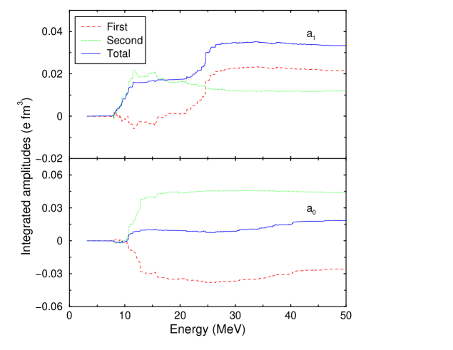
Figure 6: Integrated contributions of the first (dashed) and second (dotted) terms in the Schiff operator, together with the total contribution (solid) to diagram A, as a function of core–excitation energy with the SkO^′ interaction. The top panel is for the isovector coefficient $a_{1}$ and the bottom for the isoscalar coefficient $a_{0}$.

The type–B diagrams (see Fig. 2) are important corrections to diagram A. The effective weak isoscalar and isotensor one–body potentials (i.e. the tadpole) contribute with opposite sign from that of the isovector potential; again, see Eq. (9) of Engel et al. (2003), which displays the direct part of the one–body potential explicitly. The sign turns out to be opposite that of diagram A in the isoscalar and isotensor channels, further suppressing $a_{0}$ and $a_{2}$, and the same as diagram A in the isovector channel, largely counteracting the suppression by collectivity in that diagram. The net result for SkO^′ is in the last line of Tab. 2; for the other forces the net results appear in Tab. 3. The isovector coefficient $a_{1}$ ends up not much different from the early estimate of Ref. Flambaum et al. (1986) but the isoscalar coefficient $a_{0}$ is smaller by a factor of about 9 to 40 and the isotensor coefficient $a_{2}$ by a factor of about 7 to 16.

	$a_{0}$	$a_{1}$	$a_{2}$
SkM⋆	$0.009$	$0.070$	$0.022$
SkP	$0.002$	$0.065$	$0.011$
SIII	$0.010$	$0.057$	$0.025$
SLy4	$0.003$	$0.090$	$0.013$
SkO′	$0.010$	$0.074$	$0.018$

Table 3: Full coefficients $a_{i}$ in ${}^{199}{\rm Hg}$ for the five different Skyrme interactions used here. The units are $e~{}{\rm fm}^{3}$.

III.2 Uncertainty and final result

The several Skyrme interactions we use all give different results, but the spread in numbers is about a factor of four in the isoscalar channel, two in the isotensor channel, and much less for the large isovector coefficient $a_{1}$. It is possible that all the interactions are systematically deficient, but we have no evidence for that. In any event, the effective interaction is not the only source of uncertainty. We have evaluated only a subset of all diagrams, and although it is not obvious whether all the rest should be evaluated with effective interactions that are determined through Hartree–Fock– or RPA–based fits, there are some that should certainly be included and we would like to estimate their size.

The diagrams labeled C and D in Fig. 7 are the leading terms in bubble chains that would result from including $W$ in the Hartree–Fock calculation (C) and in the QRPA calculation (D) in ${}^{198}{\rm Hg}$. We evaluated both sets in the simple nucleus ${}^{209}{\rm Pb}$ (which has no pairing at the mean–field level), and found that diagram C can be nearly as large as the type–B diagrams in the isovector and isotensor channels. The same is true of diagram D in the isotensor channel. In that nucleus, however, diagram A is much larger than all the others and essentially determines the $a_{i}$. In ${}^{199}{\rm Hg}$, we only evaluated diagram C, but found that even though diagrams A and B can cancel there, they do so the most in the isoscalar channel, where the diagrams C and D are smallest. In the end diagram C never amounts to more than 10% of the sum of the A and B diagrams, and usually amounts to much less. Including the higher order (QRPA) terms in the bubble chain will only reduce the diagram-C contribution, so we conclude that it can be neglected. We are not positive that the same statement is true of diagram D, but unless it is much larger in ${}^{199}{\rm Hg}$ than in ${}^{209}{\rm Pb}$ (none of the other diagrams are), it can be neglected too.

The diagram labeled E represents a correction from outside our framework that is of the same order as the terms we include. We evaluated it in ${}^{209}{\rm Pb}$; it is uniformly smaller than those of type C and D. Unless the situation is very different in ${}^{199}{\rm Hg}$, it can be neglected as well. The fact that these extra diagrams are all small is not terribly surprising; they all bring in extra energy denominators and/or interrupt the collective bubble.

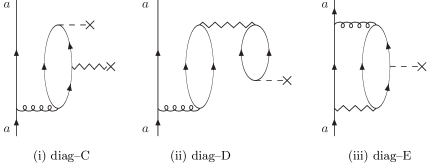
Figure 7: Diagrams we did not include in our calculation in ${}^{199}{\rm Hg}$ but the value of which we estimated through calculations in ${}^{209}{\rm Pb}$ (and ${}^{199}{\rm Hg}$ in the case of diagram C). We have omitted the labels on the the interactions; they are the same as in the earlier figures.

We have also not included the normalization factor ${\cal N}$ in Equation (6). When calculated to second order in ${}^{209}{\rm Pb}$, it is about 1.05, independent of the Skyrme interaction used. Though this factor could be larger in RPA order because of low–lying phonons, most strength is pushed up by the RPA and we do not anticipate a large increase. It is reasonable to assume these statements are true in ${}^{199}{\rm Hg}$ as well.

At short distances the NN potential is strongly repulsive and the associated short–range correlations should be taken into account. Reference Griffiths and Vogel (1991), however, reports that the correlations reduce matrix elements of the effective one–body P– and T–violating pion–exchange potential only by about 5%, and in Ref. Dobaczewski and Engel (2005), which calculates the Schiff moment of ${}^{225}{\rm Ra}$, their effects are smaller than 10%. We are not missing much by neglecting them, though we would be if we included a $\rho$–meson exchange potential.

When all is said and done, the uncertainty is dominated by our uncertainty in the effective interaction. Our preferred interaction is SkO^′, which (to repeat) gives the result

$$S_{{}^{199}{\rm Hg}}^{\rm SkO^{\prime}}~{}=~{}0.010{\rm g\bar{g}}_{0}+0.074{\rm g\bar{g}}_{1}+0.018{\rm g\bar{g}}_{2}~{}~{}~{}[e~{}{\rm fm}^{3}]~{}.$$ (14)

If instead we average the results from the five interactions, we get

$$S_{{}^{199}{\rm Hg}}^{\rm ave}~{}=~{}0.007{\rm g\bar{g}}_{0}+0.071{\rm g\bar{g}}_{1}+0.018{\rm g\bar{g}}_{2}~{}~{}~{}[e~{}{\rm fm}^{3}]~{},$$ (15)

The range of results in Tab. 3 is a measure of the uncertainty.

As noted in the introduction, Refs. Dmitriev and Sen’kov (2003); Dmitriev et al. (2005) contain a similar calculation. They report

$$S_{{}^{199}{\rm Hg}}^{\rm Ref.\ [8]}~{}=~{}0.0004{\rm g\bar{g}}_{0}+0.055{\rm g\bar{g}}_{1}+0.009{\rm g\bar{g}}_{2}~{}~{}~{}[e~{}{\rm fm}^{3}]~{},$$ (16)

the most striking aspect of which is the isoscalar coefficient $a_{0}$; it is more than an order of magnitude smaller than our preferred value and five times smaller than the smallest coefficient produced by any of our interactions. We see no fundamental reason for such serious suppression, and suspect that the same cancellation we observe is coincidentally more precise in the single Hg calculation of Refs. Dmitriev and Sen’kov (2003); Dmitriev et al. (2005). The authors applied their method to other nuclei, but did not find the same level of suppression in any of them. Even the cancellation produced in our calculations by SkP and SLy4 seems coincidentally severe. Though it is possible that other realistic Skyrme interactions would produce still smaller coefficients, we have a hard time imagining it.

IV Conclusions

Our goal has been a good calculation of the dependence of the Schiff moment of ${}^{199}{\rm Hg}$, the quantity that determines the electric dipole moment of the corresponding atom, on three P– and T–violating $\pi$NN coupling constants. The current experimental limit on the dipole moment of the ${}^{199}{\rm Hg}$ atom, $|d|<2.1\times 10^{-28}e~{}{\rm cm}$, together with the theoretical results of Ref. Dzuba et al. (2002), $d=-2.8\times 10^{-17}(S/e~{}{\rm fm}^{3})~{}e~{}{\rm cm}$, yields the constraint $|S|<7.5\times 10^{-12}e~{}{\rm fm}^{3}$. The $a_{i}$ calculated in this paper then give a constraint on the three ${\rm\bar{g}}_{i}$.

In obtaining the $a_{i}$ we have included what we believe to be most of the important physics, including a pion–exchange P– and T–violating interaction, collective effects that are known to renormalize strength distributions of Schiff–like operators, pairing at the mean–field level, self–consistency, and finally, several different Skyrme interactions. The last of these, together with an examination of effects we omitted, allows us to give the first real discussion of uncertainty for a calculation in this experimentally important nucleus.

We conclude that while the isovector coefficient $a_{1}$ is not very different from the initial estimate of Ref. Flambaum et al. (1986), the isoscalar coefficient, which determines the limit one can set on the QCD parameter $\bar{\theta}$, is smaller by between about 9 and 40 (with the former our preferred value) and the isotensor parameter $a_{2}$ by a factor between about 7 and 16 (with our preferred value about 10). The uncertainty in these numbers comes primarily from our lack of knowledge about the effective interaction. There is good reason to make better measurements of low–lying dipole strength, particularly in the isoscalar channel. They would help to unravel the details of nuclear structure that determine the Schiff moment.

V Appendix

V.1 Rules for quasiparticle diagrams in the uncoupled basis

There are some differences between our rules for quasiparticle diagrams and the usual rules for particle–hole diagrams. The main one is that one– and two–body operators are written in a quasiparticle basis and do not conserve quasiparticle number, leading to different expressions for matrix elements. An example is the generic quasiparticle operator $O_{20}$, which contains two quasiparticle creation and no destruction operators. Its matrix elements will be written $\langle kl|O_{20}|-\rangle$, which means that it creates two quasiparticle states $|k\rangle|l\rangle$ out of the quasiparticle vacuum $|-\rangle$.

In what follows, “in” refers to lines with arrows pointing toward the vertex and “out” to lines pointing away from it. A diagram should be read from top to bottom, and from left to right. The rules are then:

1. Each operator $O_{11}$ contributes $\langle{\rm out}|O_{11}|{\rm in}\rangle$;

2. Each operator $O_{20}$ contributes $\langle{\rm out,out^{\prime}}|O_{20}|-\rangle$; because the diagram is read from the left, the label “out” is on the line that is further to the left;

3. Each operator $O_{02}$ contributes $\langle-|O_{02}|{\rm in,in^{\prime}}\rangle$;

4. Each operator $O_{22}$ contributes $\langle{\rm out,out^{\prime}}|O_{22}|{\rm in,in^{\prime}}\rangle$;

5. Each operator $O_{31}$ contributes $\langle{\rm out,out^{\prime},out^{\prime\prime}}|O_{31}|{\rm in}\rangle$;

6. Each operator $O_{13}$ contributes $\langle{\rm out}|O_{13}|{\rm in,in^{\prime},in^{\prime\prime}}\rangle$;

7. Each operator $O_{40}$ contributes $\langle{\rm out,out^{\prime},out^{\prime\prime},out^{\prime\prime\prime}}|O_{40}|-\rangle$;

8. Each operator $O_{04}$ contributes $\langle-|O_{04}|{\rm in,in^{\prime},in^{\prime\prime},in^{\prime\prime\prime}}\rangle$;

9. The diagram should be summed over all intermediate states;

10. Energy denominators are evaluated by operating with $(\epsilon_{a}-H_{0})^{-1}$ between the action of every two operators in the diagram, giving $[\epsilon_{a}+\sum_{k}\epsilon_{k}]^{-1}$, where $\epsilon_{k}$ are quasiparticle energies;

11. The phase for each diagram is $(-)^{n_{l}}$, where $n_{l}$ is the number of closed loops.

12. A factor of $1/2$ is included for each pair of lines that start at the same vertex and end at the same vertex.

Folded diagrams with additional rules occur in general, but we do not discuss them here.

V.2 Matrix elements of quasiparticles operators

We first summarize some important quantities involving the quasiparticle creation and annihilation operators $q^{{\dagger}}$ and $q$, which are defined in terms of the usual particle operators $a^{{\dagger}}$ and $a$ by

$$\left\{\begin{array}[]{c}q_{k}=u_{k}a_{k}-v_{k}\tilde{a}_{k}^{{\dagger}}\\ q_{k}^{{\dagger}}=u_{k}a_{k}^{{\dagger}}-v_{k}\tilde{a}_{k}\end{array}\right.,$$ (19)

(20)

$$\left\{\begin{array}[]{c}\tilde{q}_{k}=u_{k}\tilde{a}_{k}+v_{k}a_{k}^{{\dagger}}\\ \tilde{q}_{k}^{{\dagger}}=u_{k}\tilde{a}_{k}^{{\dagger}}+v_{k}a_{k}\end{array}\right..$$ (23)

Here

$$\tilde{q}_{k}~{}\equiv~{}\tilde{q}_{l_{k}j_{k}m_{k}}~{}=~{}(-)^{l_{k}+j_{k}+m_{k}}q_{l_{k}j_{k}-m_{k}}~{}=~{}(-)^{l_{k}+j_{k}+m_{k}}q_{-k}~{}.$$ (24)

From the anti–commutation rules for $a^{{\dagger}}$ and $a$, we derive the following anti–commutation rules for the quasiparticle operators in Eq. (20)

$$\begin{array}[]{c}\{q_{k},q_{l}\}=\{q^{{\dagger}}_{k},q^{{\dagger}}_{l}\}=\{\tilde{q}_{k},\tilde{q}_{l}\}=\{\tilde{q}^{{\dagger}}_{k},\tilde{q}^{{\dagger}}_{l}\}=\{\tilde{q}_{k},q_{l}\}=\{\tilde{q}^{{\dagger}}_{k},q^{{\dagger}}_{l}\}=0\\ \{q_{k},q^{{\dagger}}_{l}\}=\{\tilde{q}_{k},\tilde{q}^{{\dagger}}_{l}\}=\delta_{kl}\\ \{\tilde{q}_{k},q^{{\dagger}}_{l}\}=(-)^{l_{k}+j_{k}+m_{k}}\delta_{-kl}\end{array}$$ (28)

Using definition (20) and properties (24) and (28), one can write a one–body operator in second quantization as

$$T=\sum_{kl}T_{kl}a^{{\dagger}}_{k}a_{l}=T_{0}+T_{11}+T_{20}+T_{02}~{},$$ (29)

where

$$T_{0} = \sum_{k}v^{2}_{k}T_{kk}~{},$$ (30)

$$T_{11} = \sum_{kl}T_{kl}(u_{k}u_{l}q^{{\dagger}}_{k}q_{l}-v_{k}v_{l}\tilde{q}^{{\dagger}}_{l}\tilde{q}_{k})~{},$$ (31)

$$T_{20} = \sum_{kl}T_{kl}u_{k}v_{l}q^{{\dagger}}_{k}\tilde{q}^{{\dagger}}_{l}~{},$$ (32)

$$T_{02} = \sum_{kl}T_{kl}u_{l}v_{k}\tilde{q}_{k}q_{l}~{}.$$ (33)

Here, the subscripts indicate the number of quasiparticle creation and annihilation operators involved. In the same way, a two–body operator takes the form

$$V = -\frac{1}{4}\sum_{klij}(V_{klij}-V_{klji})a^{{\dagger}}_{k}a^{{\dagger}}_{l}a_{i}a_{j}=-\frac{1}{4}\sum_{klij}\overline{V}_{klij}a^{{\dagger}}_{k}a^{{\dagger}}_{l}a_{i}a_{j}=$$ (34)

$$= V_{0}+V_{11}+V_{20}+V_{02}+V_{22}+V_{31}+V_{13}+V_{40}+V_{04}~{},$$

where

$$V_{0} = \frac{1}{4}\sum_{kl}\left(u_{k}v_{k}u_{l}v_{l}P_{k}P_{l}\overline{V}_{k-kl-l}+2v_{k}^{2}v_{l}^{2}\overline{V}_{klkl}\right)~{},$$ (35)

$$V_{11} = \frac{1}{2}\sum_{kli}u_{k}v_{l}u_{i}v_{i}P_{i}\overline{V}_{kli-i}\left(q^{{\dagger}}_{k}\tilde{q}_{l}+\tilde{q}^{{\dagger}}_{l}q_{k}\right)$$ (36)

$$+\mbox{}\sum_{kli}v_{k}^{2}\overline{V}_{klki}\left(u_{l}u_{i}q^{{\dagger}}_{l}q_{i}-v_{l}v_{i}\tilde{q}^{{\dagger}}_{i}\tilde{q}_{l}\right)~{},$$

$$V_{20} = \frac{1}{4}\sum_{kli}u_{i}v_{i}P_{i}\overline{V}_{kli-i}\left(u_{k}u_{l}q^{{\dagger}}_{k}q^{{\dagger}}_{l}+v_{k}v_{l}\tilde{q}^{{\dagger}}_{l}\tilde{q}^{{\dagger}}_{k}\right)$$ (37)

$$+\mbox{}\sum_{kli}u_{k}v_{l}^{2}v_{i}\overline{V}_{klil}q^{{\dagger}}_{k}\tilde{q}^{{\dagger}}_{i},$$

$$V_{22} = \frac{1}{4}\sum_{klij}\overline{V}_{klij}\left(u_{k}u_{l}u_{i}u_{j}q^{{\dagger}}_{k}q^{{\dagger}}_{l}q_{j}q_{i}+v_{k}v_{l}v_{i}v_{j}\tilde{q}^{{\dagger}}_{j}\tilde{q}^{{\dagger}}_{i}\tilde{q}_{k}\tilde{q}_{l}\right)$$ (38)

$$+\mbox{}\sum_{klij}u_{k}v_{l}u_{j}v_{i}\overline{V}_{klij}q^{{\dagger}}_{k}\tilde{q}^{{\dagger}}_{i}\tilde{q}_{l}q_{j}~{},$$

$$V_{31} = \frac{1}{2}\sum_{klij}u_{k}v_{l}\overline{V}_{klij}\left(u_{i}u_{j}q^{{\dagger}}_{i}q^{{\dagger}}_{j}\tilde{q}^{{\dagger}}_{l}q_{k}+v_{i}v_{j}q^{{\dagger}}_{k}\tilde{q}^{{\dagger}}_{j}\tilde{q}^{{\dagger}}_{i}\tilde{q}_{l}\right)~{},$$ (39)

$$V_{40} = \frac{1}{4}\sum_{klij}u_{k}u_{l}v_{i}v_{j}\overline{V}_{klij}q^{{\dagger}}_{k}q^{{\dagger}}_{l}\tilde{q}^{{\dagger}}_{j}\tilde{q}^{{\dagger}}_{i}~{},$$ (40)

with $P_{k}=(-)^{l_{k}+j_{k}+m_{k}}$, $V_{ba}=(V_{ab})^{\dagger}$ and $\overline{V}_{abcd}=V_{abcd}-V_{abdc}$.

The matrix elements of quasiparticle operators are related to those of the usual one– and two–body operators. We show how this works for the operator $T_{20}$; the generalization to other operators follows automatically. $T_{20}$ adds two quasiparticles to any state. From $|ij\rangle=q^{{\dagger}}_{i}q^{{\dagger}}_{j}|-\rangle$ and Eq. (32), we write

$$\langle ij|T_{20}|-\rangle~{}=~{}\sum_{kl}T_{kl}u_{k}v_{l}\langle-|q_{j}q_{i}q^{{\dagger}}_{k}\tilde{q}^{{\dagger}}_{l}|-\rangle~{}.$$ (41)

Since

$$\langle-|q_{j}q_{i}q^{{\dagger}}_{k}\tilde{q}^{{\dagger}}_{l}|-\rangle~{}=~{}P_{l}[-\delta_{jk}\delta_{-li}+\delta_{-lj}\delta_{ik}]~{},$$ (42)

Eq. (41) becomes

$$\langle ij|T_{20}|-\rangle~{}=~{}-P_{i}u_{j}v_{i}\langle j|T|-i\rangle+P_{j}u_{i}v_{j}\langle i|T|-j\rangle~{}.$$ (43)

References

- Romalis et al. (2001) M. V. Romalis, W. C. Griffith, J. P. Jacobs, and E. N. Fortson, Phys. Rev. Lett. 86, 2505 (2001).
- Schiff (1963) L. I. Schiff, Phys. Rev. 132, 2194 (1963).
- Herczeg (1988) P. Herczeg, in Tests of Time Reversal Invariance in Neutron Physics (World Scientific, Singapore, New Jersey, Hong Kong, 1988), n. R. Rogerson, C. R. Gould, and J. D. Bowman, eds., page 24.
- Griffiths and Vogel (1991) A. Griffiths and P. Vogel, Phys. Rev. C 44, 1195 (1991).
- Towner and Hayes (1994) I. S. Towner and A. C. Hayes, Phys. Rev. C 49, 2391 (1994).
- Flambaum et al. (1986) V. V. Flambaum, I. B. Khriplovich, and O. P. Sushkov, Nucl. Phys. A449, 750 (1986).
- Flambaum and Ginges (2002) V. V. Flambaum and J. S. M. Ginges, Phys. Rev. A 65, 032113 (2002).
- Dmitriev and Sen’kov (2003) V. F. Dmitriev and R. A. Sen’kov, Phys. Atom. Nucl. 66, 1940 (2003).
- Dmitriev et al. (2005) V. F. Dmitriev, R. A. Sen’kov, and N. Auerbach (2005).
- Brown (1970) G. E. Brown, in Facets of Physics (Academic Press, New York, 1970), d. Allen Bromley and Vernon W. Hughes, eds.
- Ellis and Osnes (1997) P. J. Ellis and E. Osnes, Rev. Mod. Phys. 1997, 777 (1997).
- Bender et al. (2002) M. Bender, J. Dobaczewski, J. Engel, and W. Nazarewicz, Phys. Rev. C 65, 054322 (2002).
- Sushkov et al. (1984) O. P. Sushkov, V. V. Flambaum, and I. B. Khriplovich, Sov. Phys. JETP 60, 873 (1984).
- Terasaki et al. (2005) J. Terasaki, J. Engel, M. Bender, J. Dobaczewski, W. Nazarewicz, and M. Stoitsov, Phys. Rev. C 71, 034310 (2005).
- Agrawal et al. (2003) B. Agrawal, S. Shlomo, and A. Sanzhur, Phys. Rev. C 67, 034314 (2003).
- Reinhard et al. (1999) P.-G. Reinhard, D. J. Dean, W. Nazarewicz, J. Dobaczewski, J. A. Maruhn, and M. R. Strayer, Phys. Rev. C 60, 014316 (1999).
- Engel et al. (2003) J. Engel, M. Bender, J. Dobaczewski, J. H. de Jesus, and P. Olbratowski, Phys. Rev. C 68, 025501 (2003).
- Beiner et al. (1975) M. Beiner, H. Flocard, N. V. Giai, and P. Quentin, Nucl. Phys. A238, 29 (1975).
- Bartel et al. (1982) J. Bartel, P. Quentin, M. Brack, C. Guet, and H. B. Håkansson, Nucl. Phys. A386, 79 (1982).
- Chabanat et al. (1998) E. Chabanat, P. Bonche, P. Haensel, J. Meyer, and R. Schaeffer, Nucl. Phys. A635, 231 (1998), Nucl. Phys. A643, 441(E) (1998).
- Dobaczewski et al. (1984) J. Dobaczewski, H. Flocard, and J. Treiner, Nucl. Phys. A 422, 103 (1984).
- Clark et al. (2001) H. L. Clark, Y.-W. Lui, and D. H. Youngblood, Phys. Rev. C 63, 031301(R) (2001).
- Davis et al. (1997) B. F. Davis et al., Phys. Rev. Lett. 79, 609 (1997).
- Hamamoto et al. (1998) I. Hamamoto, H. Sagawa, and X. Z. Zhang, Phys. Rev. C 57, R1064 (1998).
- Colò et al. (2000) G. Colò, N. V. Giai, P. F. Bortignon, and M. R. Quaglia, Phys. Lett. B485, 362 (2000).
- Vretenar et al. (2000) D. Vretenar, A. Wamdelt, and P. Ring, Phys. Lett. B487, 334 (2000).
- Abrosimov et al. (2002) V. I. Abrosimov, A. Dellafiore, and F. Matera, Nucl. Phys. A697, 748 (2002).
- Shlomo and Sanzhur (2002) S. Shlomo and A. Sanzhur, Phys. Rev. C 65, 044310 (2002).
- Engel et al. (1999) J. Engel, J. L. Friar, and A. C. Hayes, Phys. Rev. C 61, 035502 (1999).
- Dobaczewski and Engel (2005) J. Dobaczewski and J. Engel, Submmitted to Phys. Rev. Lett. (2005).
- Dzuba et al. (2002) V. A. Dzuba, V. V. Flambaum, J. S. M. Ginges, and M. G. Kozlov, Phys. Phys. A 66, 012111 (2002).