Coordinates, modes and maps for the density functional

Abstract

Special bases of orthogonal polynomials are defined, that are suited to expansions of density and potential perturbations under strict particle number conservation. Particle-hole expansions of the density response to an arbitrary perturbation by an external field can be inverted to generate a mapping between density and potential. Information is obtained for derivatives of the Hohenberg-Kohn functional in density space. A truncation of such an information in subspaces spanned by a few modes is possible. Numerical examples illustrate these algorithms.

I Introduction

The well-known Hohenberg-Kohn (HK) density functional [1] and its finite temperature generalization by Mermin [2] suffer from the absence of constructive algorithms after their respective existence theorems. The Thomas-Fermi (TF) approach, however, and related developments such as [3], [4], have gone a long way into creating functionals with practical physical values. For reviews on the effectiveness of the detailed forms of the functional found empirically, see for instance [5] and [6]. For applications of Skyrme forces to nuclear densities, see for instance [7] and [8].

Standard perturbation theories (particle hole hierarchy of excitations, configuration mixing, generator coordinates, etc.), extrapolating from well understood mean field theories, give a constructive approach to the intricacies of a true ground state (GS), at the well known heavy cost of calculations with many degrees of freedom. But such theories proved to be practical, because suitable truncations were found that restricted calculations to few modes, collective or not, subspaces with fewer degrees of freedom. The purpose of the present note is to attempt answering a similar question in the space of densities rather than the space of wave functions: are there possible truncations, is there a possibility to restrict the functional to a set of few density modes?

For this we visit again the fundamentals of the HK functional $F[\rho]$ in a systematic approach, based upon the following chain of arguments,

i) given the full Hamiltonian, $H=T+V+U,$ with a fixed kinetic operator $T=\sum_{i}t_{i},$ a fixed two-body potential operator $V=\sum_{i>j}v_{ij},$ and a variable one-body potential operator $U=\sum_{i}u_{i},$ assume a non degenerate, square normalized GS $\Psi,$ with its corresponding eigenvalue $E,$ density $\rho$ and functional $F[\rho]\equiv\langle\Psi|(T+V)|\Psi\rangle=E-\langle\Psi|U|\Psi\rangle;$ find the functional derivatives $\delta\rho/\delta u$ and, considering first $F$ as a functional of $u$ rather than $\rho,$ find $\delta F/\delta u,$

ii) expand such functional derivatives into suitable bases, to describe them by convenient matrices and vectors,

iii) then invert $\delta\rho/\delta u$ to know $\delta u/\delta\rho,$

iv) furthermore obtain $\delta F/\delta\rho$ by eliminating $\delta u$ between $\delta F/\delta u$ and $\delta u/\delta\rho;$ further information about $F$ might be obtained by integrating $\delta F/\delta\rho,$ or by comparing with phenomenological approaches, such as gradient expansions,

v) at each stage, try a compression of the information, by a truncation of the theory to a few “density modes”.

A preliminary question is in order, however: can this formal program be carried if particle number is conserved in the mean only, as occurs with Lagrange multiplier techniques? According to [5], the chemical potential, as a function of a continuous particle number, shows derivative discontinuities. We thus find it safer, in this paper, to stick to “slices” of the functional, those for fixed, integer particle numbers. We also restrict our considerations to pure eigenstates of $H,$ at zero temperature.

In Section II, we carry the program in the absence of $V;$ the trivially soluble situation of independent fermions allows us to easily describe the mapping, $\rho\leftrightarrow u,$ for both infinitesimal and finite variations of $u.$ In Section III we reinstate $V,$ but use the Hartree-Fock (HF) approximation to still obtain $\rho$ without excessive technical complications. Section IV is dedicated to a better understanding of the “tangent” mapping $\delta\rho/\delta u$ [9] when full correlations are present. Then Section V introduces, via a new family of orthogonal polynomials, candidates for density and potential space modes, that might allow a compacted description of the functional and its $\rho\leftrightarrow u$ mapping. An investigation of the relevance of such modes is provided numerically, for a toy model of independent fermions. The numerical investigation is continued in Section VI, by means of a second toy model, with now correlated fermions. Section VII contains a discussion and a conclusion.

II Particle-hole expansions for independent fermions

Let $Z$ be the particle number for a finite Fermion system. For simplicity we ignore discrete labels such as spins and isospins. Set $v=0,$ temporarily, the case of two-body forces being discussed later. The one-body potential function $u$ is taken here as a local potential $u(r).$ The Hamiltonian then boils down to $H=\sum_{i=1}^{Z}(t_{i}+u_{i})$ and its GS, assumed to be non degenerate, is a Slater determinant. The HK functional, in this special case, reduces to the kinetic expectation value, $\langle\Psi|T|\Psi\rangle.$

Consider a perturbation $\delta u$ of the local potential $u.$ We find it practical to expand it in an orthonormal basis of functions $w_{\alpha}(r),$ namely $\delta u(r)=\sum_{\alpha=1}^{\infty}w_{\alpha}(r)\,\delta u_{\alpha}.$ According to the HK theorem [1], this basis must be orthogonal to a “flat potential component” $w_{0}(r)=1.$ This is satisfied if we find a basis such that, $\forall\alpha>0,\,\int dr\,w_{\alpha}(r)=0.$ It is then understood that the index $\alpha$ will run from $1$ to $\infty.$ For obvious practical reasons, however, the expansion will sooner or later be truncated at some finite rank of the basis.

The perturbation $\delta u$ induces a perturbation $\delta\rho$ of the density of the GS $\Psi$ of $H,$ and we find it convenient to expand $\delta\rho$ in the same orthonormal basis $\{w_{\beta}(r)\},$ namely $\delta\rho(r)=\sum_{\beta=1}^{\infty}w_{\beta}(r)\,\delta\rho_{\beta}.$ The fact that this basis satisfies the constraint, $\forall\beta>0,\ \int dr\,w_{\beta}(r)=0,$ is very useful because $\delta\rho$ does not change the particle number, namely $\delta\rho$ automatically satisfies the condition $\int dr\,\delta\rho(r)=0.$ It is very convenient that the constraint of particle number conservation and that of “non constant potential variation” allow the same choice for our forthcoming basis $\{w_{\alpha}\}.$

A trivial particle-hole argument then provides that perturbation $\delta\Psi$ induced by $\delta u.$ Let the “hole index” $i=1,...,Z$ and “particle index” $I$ (running from $Z+1$ to $\infty$) denote occupied and empty orbitals, respectively, with the corresponding single particle energies $\eta_{i}$ and $\eta_{I}$ and orthonormal wave functions $\psi_{i}$ and $\psi_{I}.$ For the sake of simplicity in the following, such orbital wave functions $\psi(r)$ are assumed to be real in the coordinate representation. Each filled orbital picks a variation $\delta\psi_{i}(r)=\sum_{I}\psi_{I}(r)\,\langle I|\delta u|i\rangle/(\eta_{i}-\eta_{I}).$ Hence,

$$\delta\rho(r)=2\sum_{iI}\,\psi_{i}(r)\psi_{I}(r)\,\frac{\langle I|\delta u|i\rangle}{\eta_{i}-\eta_{I}}\,.$$ (1)

This reads, when $\delta u$ and $\delta\rho$ are expanded,

$$\delta\rho_{\beta}=2\sum_{iI\alpha}{\cal D}_{\beta iI}\,\frac{\langle I|w_{\alpha}|i\rangle}{\eta_{i}-\eta_{I}}\,\delta u_{\alpha}\,,$$ (2)

where ${\cal D}$ denotes the projection of a particle-hole product of orbitals upon the basis $\{w_{\alpha}\},$

$${\cal D}_{\beta iI}=\int dr\,w_{\beta}(r)\,\psi_{i}(r)\,\psi_{I}(r).$$ (3)

Note, incidentally, that particle-hole orthonormality ensures that, $\forall iI,$ $\int dr\,\psi_{i}(r)\psi_{I}(r)=0.$ Hence, functions $w_{\alpha}$ expanded in the basis of particle-hole products $\psi_{i}\,\psi_{I},$ a basis to be orthonormalized, automatically fulfill the requested condition for $\delta u$ and $\delta\rho.$ Furthermore, positivity of the density is guaranteed as variations $\delta\rho$ in Eq. (1) are based on variations of the wave function, in particular by particle-hole admixtures to the GS determinant $\Psi.$

Define the matrix,

$${\cal N}_{\beta\alpha}=2\sum_{iI}{\cal D}_{\beta iI}\,\frac{\langle I|w_{\alpha}|i\rangle}{\eta_{i}-\eta_{I}}\,.$$ (4)

Notice also that the perturbation matrix element, $\langle I|w_{\alpha}|i\rangle,$ coming from $\delta u,$ is nothing but an integral of a three term product, amounting to ${\cal D}_{\alpha iI}.$ Notice finally that the energy denominators correspond to a propagator $G=Q(E-QHQ)^{-1}Q,$ if Q is the particle-hole space projector. This operator is diagonal in the particle-hole space, obviously. Then, in a condensed notation, ${\cal N}=2\,{\cal D}\,G\,\tilde{\cal D},$ where the tilde denotes transposition between index $\alpha$ and pair index $iI.$ Consider now $\delta\rho$ and $\delta u$ as just vectors with components $\delta\rho_{\beta}$ and $\delta u_{\alpha},$ respectively, sooner or later truncated. Since Eq. (2) reads $\delta\rho={\cal N}\delta u,$ the HK theorem states that, under the usual condition of non degeneracy for the GS of $H,$ an inversion is possible. Namely for any $\delta\rho$ which leaves $\rho+\delta\rho$ in the manifold of actual densities, there exists a unique $u+\delta u,$ provided $\delta u$ does not add a constant component to $u.$ Under such precautions, the infinite matrix ${\cal N}$ can be inverted, and the same can be expected under “reasonable” truncations of ${\cal N}.$ Accordingly, while Eq. (2) provides the functional derivative $\delta\rho/\delta u,$ one obtains the functional derivative $\delta u/\delta\rho,$

$$\delta u_{\alpha}=\sum_{\beta}\left({\cal N}^{-1}\right)_{\alpha\beta}\delta\rho_{\beta}\,.$$ (5)

Now, that variation $\delta E$ of the GS energy induced by $\delta u$ is trivial. It just reads,

$$\delta E=\langle\Psi|\delta U|\Psi\rangle,$$ (6)

because of the stationarity of the GS energy with respect to $\delta\Psi.$ Accordingly, for the functional under study,

$$\delta F=\delta E-\delta\langle\Psi|U|\Psi\rangle=-\langle\delta\Psi|U|\Psi\rangle-\langle\Psi|U|\delta\Psi\rangle=-2\langle\Psi|U|\delta\Psi\rangle=-2\langle\Psi|U\,G\,\delta U|\Psi\rangle,$$ (7)

hence,

$$\delta F=-2\sum_{iI}\langle i|u|I\rangle\,(\eta_{i}-\eta_{I})^{-1}\,\langle I|\delta u|i\rangle,$$ (8)

and finally, with proper expansions,

$$\delta F=-2\sum_{iI}\langle i|u|I\rangle\,(\eta_{i}-\eta_{I})^{-1}\,\sum_{\alpha}{\cal D}_{\alpha iI}\sum_{\beta}\left({\cal N}^{-1}\right)_{\alpha\beta}\delta\rho_{\beta}\,.$$ (9)

It may be convenient here to set from $u$ a column vector ${\cal U}$ with components

$${\cal U}_{\,iI}=\int dr\,u(r)\,\psi_{i}(r)\,\psi_{I}(r),$$ (10)

hence the functional derivative $\delta F/\delta\rho$ reads, in a condensed, matrix and vector notation,

$$\delta F=-\,\tilde{\cal U}\,G\,\tilde{\cal D}\,\left({\cal D}\,G\,\tilde{\cal D}\right)^{-1}\,\delta\rho.$$ (11)

This simplifies if one observes that, because of orthogonality between particle and hole orbitals, the product $\psi_{i}(r)\,\psi_{I}(r)$ can be expanded in the $w$-basis as,

$$\psi_{i}(r)\,\psi_{I}(r)=\sum_{\beta}{\cal D}_{iI\beta}\,w_{\beta}(r).$$ (12)

Accordingly,

$${\cal U}_{iI}=\int dr\,u(r)\,\sum_{\beta}{\cal D}_{iI\beta}\,w_{\beta}(r)=\sum_{\beta}u_{\beta}\,{\cal D}_{iI\,\beta},$$ (13)

with $u_{\beta}$ the components of $u$ in our special basis. Combining Eqs. (11) and (13) results in

$$\delta F=-\sum_{\alpha\beta\gamma}u_{\beta}\left({\cal D}\,G\,\tilde{\cal D}\right)_{\beta\gamma}\,\left[\left({\cal D}\,G\,\tilde{\cal D}\right)^{-1}\right]_{\gamma\alpha}\,\delta\rho_{\alpha}=-\sum_{\alpha}u_{\alpha}\,\delta\rho_{\alpha}.$$ (14)

This avoids the transition between different bases through the matrix ${\cal D}.$ One thus recovers the trivial result, $\delta F=-\int dr\,u(r)\,\delta\rho(r),$ but it must be kept in mind that, here, $u$ has become a functional of $\rho.$ Whether this simplification is made or not, this makes a set of numerical, non linear, coupled, partial differential equations relating $F$ and $\rho.$ The non linearity comes in particular from the orbitals and single particle energies which occur in the definition of ${\cal N}.$ We stress again that the vector, $\tilde{\cal U}\,{\cal D}^{-1},$ just makes an “$\alpha$” representation of $u,$ converted from its particle-hole representation ${\cal U}.$

A comment about Legendre transforms is here in order [9]. According to the Hellmann-Feynman theorem, $\delta E/\delta u=\rho.$ But then, $F\equiv E-\int dr\,u(r)\,\rho(r)$ is nothing but the Legendre transform of $E$ and the primary degree of freedom is not $u$ any more, but $\rho.$ Note that the reasoning remains if $V$ is reinstated. In all cases, $u$ is recovered from $\delta F/\delta\rho=-u.$

For Eq. (11), and its generalization if two-body forces are present, to become a tool to obtain information about $F,$ dynamical models are obviously necessary. These are the subjects of several of the forthcoming sections.

III Two-body forces and Hartree-Fock model

In this section, we stay with $Z$ fermions, but reinstate in the Hamiltonian the two-body interaction $v_{ij}$ with the operator $V=\sum_{i>j=1}^{Z}v_{ij}.$ The HK functional is $\langle\Psi|(T+V)|\Psi\rangle.$ While a Slater determinant $\Psi$ was available as the true GS of a simpler $H=T+U$ in the previous section, we cannot usually obtain the true GS with two-body forces present in a full $H=T+V+U.$ Thus, in this section, we tolerate for $\Psi$ the HF ground state of $H,$ with energy $E_{0},$ and furthermore assume that this HF approximation does not create degeneracies between distinct $\Psi$’s. Under this precaution of uniqueness, there exists an extension of the HK theorem. Indeed, in the space of Slater determinants, let $\Psi$ and $\Psi^{\prime}$ be the HF GSs of $H=T+V+U$ and $H^{\prime}=T+V+U^{\prime},$ respectively, and let $\rho(r)$ and $\rho^{\prime}(r)$ be their respective densities. The two Hamiltonians differ by their (local) one-body operators $U=\sum_{i=1}^{Z}u(r_{i})$ and $U^{\prime}=\sum_{i=1}^{Z}u^{\prime}(r_{i})$ only. Their HF GS energies $E_{0}=\langle\Psi|H|\Psi\rangle$ and $E^{\prime}_{0}=\langle\Psi^{\prime}|H^{\prime}|\Psi^{\prime}\rangle,$ non degenerate, may be equal or distinct. Now, if $\rho$ and $\rho^{\prime}$ were equal, then the usual HK arguments, namely $E_{0}^{\prime}-E_{0}<\langle\Psi|(H^{\prime}-H)|\Psi\rangle=\int dr\,[u^{\prime}(r)-u(r)]\,\rho(r)$ and $E_{0}-E_{0}^{\prime}<\langle\Psi^{\prime}|(H-H^{\prime})|\Psi^{\prime}\rangle=\int dr\,[u(r)-u^{\prime}(r)]\,\rho(r),$ necessarily lead to $\rho\neq\rho^{\prime},$ by contradiction.

It can be stressed here that, again because of the stationarity of the energy with respect to variations of $\Psi,$ we can still take advantage of Eq. (6) for the variation of the energy induced by a variation $\delta u.$ This reads, with notations already used in the previous section,

$$\delta E_{0}=\langle\Psi|\delta U|\Psi\rangle\,.$$ (15)

The same holds every time we approximate the GS by means of the Rayleigh-Ritz principle in a restricted space of wave functions. As a general consequence, we obtain again Eq. (7), namely, $\delta F=-2\langle\Psi|U|\delta\Psi\rangle,$ for every such variational approximation of $\Psi.$

That variation of $\delta\Psi$ induced by $\delta u$ is slightly more complicated, in the HF case, than in the trivial case of Section II where $H=T+U.$ Indeed, each filled orbital is driven by the perturbed HF equation,

$$[\eta_{i}+\delta\eta_{i}-u(r)-\delta u(r)]\,[\psi_{i}(r)+\delta\psi_{i}(r)]+\frac{\hbar^{2}}{2m}\,\Delta_{r}\,[\psi_{i}(r)+\delta\psi_{i}(r)]\,=$$ (16)

$$\sum_{j=1}^{Z}\int dr^{\prime}\,v(r-r^{\prime})\,[\psi_{j}(r^{\prime})+\delta\psi_{j}(r^{\prime})]^{2}\,[\psi_{i}(r)+\delta\psi_{i}(r)]\,-$$ (17)

$$\sum_{j=1}^{Z}\int dr^{\prime}\,v(r-r^{\prime})\,[\psi_{j}(r^{\prime})+\delta\psi_{j}(r^{\prime})]\,[\psi_{i}(r^{\prime})+\delta\psi_{i}(r^{\prime})]\,[\psi_{j}(r)+\delta\psi_{j}(r)]\,.$$ (18)

The non locality of the HF mean field, because of antisymmetrization, is written in an explicit way in the right-hand side above, in the coordinate representation. An equivalent form of this perturbed HF Eq. (18) is obtained if we retain its first order terms only and consider the particle-hole infinitesimal components $\delta c_{iI},$ again assumed here to be real numbers,

$$(\eta_{i}-\eta_{I})\,\delta c_{iI}-\langle I|\delta u|i\rangle=\sum_{jJ}\,[\langle IJ|v|ij\rangle+\langle Ij|v|iJ\rangle]\,\delta c_{jJ}.$$ (19)

Thus $\psi_{i}(r)$ becomes $\psi_{i}(r)+\sum_{I}\psi_{I}(r)\,\delta c_{iI}.$ Notice that $\delta\eta_{i}$ drops out from the calculation, as should be expected. Then define in particle-hole space the symmetric matrix, with antisymmetrized matrix elements of $v,$

$$A_{(iI)(jJ)}=(\eta_{i}-\eta_{I})\delta_{ij}\delta_{IJ}-\langle IJ|v|ij\rangle-\langle Ij|v|iJ\rangle.$$ (20)

Here $\delta$ is a Kronecker symbol and we must use pairwise indices $(iI)$ when defining the inverse $A^{-1}$ to be used; this $A^{-1}$ generalizes the propagator used in Eq. (4), and thus,

$$\delta c_{iI}=\sum_{jJ}\left(A^{-1}\right)_{(iI)(jJ)}\,\langle J|\delta u|j\rangle.$$ (21)

This leads to the variation $\delta\rho,$ and the analog of Eq. (2) reads,

$$\delta\rho_{\beta}=2\sum_{(iI)(jJ)\alpha}{\cal D}_{\beta iI}\,\left(A^{-1}\right)_{(iI)(jJ)}\,\langle J|w_{\alpha}|j\rangle\,\delta u_{\alpha},$$ (22)

where the overlap matrix ${\cal D}$ is the same as defined in the previous section. Actually, this boils down to the even simpler formula, in matrix and vector notations,

$$\delta\rho=2\,{\cal D}\,A^{-1}\,\tilde{\cal D}\,\delta u,$$ (23)

where the tilde again denotes transposition of that connection ${\cal D}$ between the particle-hole products $\psi_{i}(r)\psi_{I}(r)$ and their rearrangement into an orthonormal basis $\{w_{\alpha}(r)\}.$ Note, incidentally, that, if $v=0,$ the matrix ${\cal F}\equiv 2\,{\cal D}\,A^{-1}\,\tilde{\cal D}$ boils down to the matrix ${\cal N},$ which is obviously negative semidefinite. We even expect ${\cal N}$ to be negative definite. The same is expected for ${\cal D}\,A^{-1}\,\tilde{\cal D}.$ The stability of our HF solutions is assumed as long, at least, as $v$ is a weak enough interaction, and this “definiteness” of ${\cal F}$ is intuitively most likely.

In the following, we shall also need the inverse of ${\cal F}.$ The final result for the variation of $F$ reads,

$$\delta F=-\,\tilde{\cal U}\,A^{-1}\,\tilde{\cal D}\,\left[\,{\cal D}\,A^{-1}\,\tilde{\cal D}\,\right]^{-1}\delta\rho,$$ (24)

and, like in Section II, this expression, in a transparent notation, reads $\delta F=-\sum_{\alpha}u_{\alpha}\,\delta\rho_{\alpha}.$ For obvious reasons of numerical convergence, the number of needed $w_{\alpha}$ states must be large enough to overlap a sufficient number of particle-hole components of $\delta\rho.$ But as will be found in the coming numerical applications, a surprisingly small number of $w_{\alpha}$ states might sometimes be sufficient.

IV Symmetry of the density-potential mapping in general

With the exact ground energy $E$ and exact GS $\Psi$ of a full $H=T+V+U,$ and $Q=1-|\Psi\rangle\langle\Psi|$ the projector out of $\Psi,$ the Brillouin-Wigner perturbation theory gives the exact result for first order functional derivatives,

$$|\delta\Psi\rangle=\frac{Q}{E-QHQ}\,\delta U\,|\Psi\rangle=\sum_{n=1}^{\infty}|\Psi_{n}\rangle\,\frac{\langle\Psi_{n}|\delta U|\Psi\rangle}{E-E_{n}}\,.$$ (25)

We assume here that a resolution of the identity with real numbers and reasonable truncations, convenient for numerics, are available. The sum over excited states $\Psi_{n}$ includes integrals over the continuum, if necessary. Let us single out the first of our identical particles and integrate out all the other ones, to define the following transition densities,

$$\Theta_{n}(r)=\int dr_{2}\,dr_{3}\,...\,dr_{Z}\,\Psi_{n}(r,r_{2},r_{3},...,r_{Z})\,\Psi(r,r_{2},r_{3},...,r_{Z}).$$ (26)

Notice that, from its very definition, $\Theta_{n}$ integrates out to $0,$ namely $\int dr\ \Theta_{n}(r)=0.$ Hence $\Theta_{n}$ can be represented in the $w$-basis without any loss of information.

Since $\delta U=\sum_{i=1}^{Z}\delta u(r_{i})$ is a symmetric operator, it is clear that Eq. (25) also reads,

$$|\delta\Psi\rangle=\sum_{n=1}^{\infty}|\Psi_{n}\rangle\,\frac{Z\int dr\,\delta u(r)\,\Theta_{n}(r)}{E-E_{n}}=\sum_{n\,\alpha}|\Psi_{n}\rangle\,\frac{Z\int dr\,w_{\alpha}(r)\,\Theta_{n}(r)}{E-E_{n}}\,\delta u_{\alpha}\,,$$ (27)

where we have again expanded $\delta u$ in the basis $\{w\}.$ There pops out a matrix,

$$D_{\alpha\,n}=Z\int dr\,w_{\alpha}(r)\,\Theta_{n}(r),$$ (28)

as a generalization of the matrix ${\cal D}_{\alpha\,iI}.$

Now, by definition, the density of the GS is,

$$\rho(r)=Z\int dr_{2}\,dr_{3}\,...\,dr_{Z}\,\left[\Psi(r,r_{2},r_{3},...,r_{Z})\right]^{2},$$ (29)

and its variation is,

$$\delta\rho(r)=2Z\int dr_{2}\,dr_{3}\,...\,dr_{Z}\,\Psi(r,r_{2},r_{3},...,r_{Z})\,\delta\Psi(r,r_{2},r_{3},...,r_{Z}).$$ (30)

This becomes, if one replaces $\delta\Psi$ by its expression, Eq. (27),

$$\delta\rho(r)=2Z\sum_{n\,\alpha}\Theta_{n}(r)\,\frac{D_{\alpha\,n}}{E-E_{n}}\,\delta u_{\alpha}.$$ (31)

An expansion of $\delta\rho$ in the $\{w\}$ basis gives its coordinates,

$$\delta\rho_{\beta}=2\,\sum_{n\,\alpha}D_{\beta\,n}\,\frac{1}{E-E_{n}}\,D_{\alpha\,n}\,\delta u_{\alpha},$$ (32)

hence, in an obvious notation, a symmetric “flexibility” matrix ${\cal F}=2\,D\,G\,\tilde{D}$ connecting $\delta u$ and $\delta\rho.$ In hindsight, the symmetry of ${\cal F}$ (and of its approximations under the Rayleigh-Ritz variational principle) is straightforward. Indeed, since $u=-\,\delta F/\delta\rho,$ then $\delta u_{\alpha}/\delta\rho_{\beta}=-\,\delta^{2}F/(\delta\rho_{\alpha}\,\delta\rho_{\beta}).$ All denominators $E-E_{n}$ being negative definite, the negative definite nature of this exact ${\cal F}$ is also transparent.

We conclude this section on the general case with explicit expressions for $\delta F/\delta\rho$ and $\delta^{2}F/(\delta\rho\delta\rho^{\prime}).$ With Eqs. (27), (28) the general form for $\delta F,$ see Eq. (7), reads

$$\delta F=-2\langle\Psi|U|\delta\Psi\rangle=-2\sum_{n\alpha}\langle\Psi|U|\Psi_{n}\rangle\,(E-E_{n})^{-1}D_{\alpha n}\,\delta u_{\alpha}=-2\sum_{n\alpha}{\cal U}_{n}\,(E-E_{n})^{-1}D_{\alpha n}\,\delta u_{\alpha}.$$ (33)

Here the numbers

$${\cal U}_{n}=\int dr\,\langle\Psi|\left[\sum_{i=1}^{Z}u(r_{i})\right]|\Psi_{n}\rangle=Z\int dr\,u(r)\,\Theta_{n}(r),$$ (34)

are now the components of $u$ in the space of transition densities, generalizing Eq. (10) for states $\Psi,$ $\Psi_{n}$ containing correlations. Upon inverting Eq. (32) we find, as a generalization of Eq. (24),

$$\delta F=-\,\tilde{\cal U}\,G\,\tilde{D}\,\left[\,D\,G\,\tilde{D}\,\right]^{-1}\delta\rho.$$ (35)

This simplifies if we expand

$$\Theta_{n}(r)=Z^{-1}\sum_{\beta}D_{n\beta}\,w_{\beta}(r).$$ (36)

Then

$${\cal U}_{n}=\int dr\,u(r)\sum_{\beta}D_{n\beta}\,w_{\beta}(r)=\sum_{\beta}u_{\beta}\,D_{n\beta},$$ (37)

with again the components of $u$ in our special $w$-basis, $u_{\beta}=\int dr\,u(r)\,w_{\beta}(r).$ Accordingly,

$$\left[\tilde{\cal U}\,G\,\tilde{D}\right]_{\gamma}=\sum_{\beta n}u_{\beta}\,D_{\beta n}\,G_{nn}\,\tilde{D}_{n\gamma}=\frac{1}{2}\sum_{\beta}u_{\beta}\,{\cal F}_{\beta\gamma},$$ (38)

hence finally, as expected,

$$\delta F=-\sum_{\alpha\beta\gamma}u_{\beta}\,{\cal F}_{\beta\gamma}\,\left[{\cal F}^{-1}\right]_{\gamma\alpha}\,\delta\rho_{\alpha}=-\sum_{\alpha}u_{\alpha}\,\delta\rho_{\alpha},$$ (39)

as before in sections II and III. Similarly, the second derivative of $F$ is found directly from the inverse of Eq. (32),

$$\delta^{2}F/(\delta\rho_{\alpha}\delta\rho_{\beta})=-\left({\cal F}^{-1}\right)_{\alpha\beta}=-\left[\left(2DG\tilde{D}\right)^{-1}\right]_{\alpha\beta}.$$ (40)

Hence, from Eqs. (35) and (40),

$$\delta F/\delta\rho_{\alpha}=2\sum_{\beta}\left(\tilde{\cal U}G\tilde{D}\right)_{\beta}\ \delta^{2}F/(\delta\rho_{\beta}\delta\rho_{\alpha}),$$ (41)

another useful equation to test phenomenological functionals $F[\rho],$ by calculating quantities such as $\tilde{\cal U}G\tilde{D}$ from microscopic wave functions and energies for simple systems.

V One dimensional toy model, special polynomials

Assume that $r$ is just one dimensional, running from $-\infty$ to $\infty.$ Define $t=-d^{2}/(2dr^{2}),$ with a nucleon mass $m=1,$ $\hbar=1$ and $p=-id/dr.$ In the present section, we are first interested in the Hamiltonian $H_{0}=\sum_{i=1}^{Z}(p_{i}^{2}/2+r_{i}^{2}/2);$ it is not a bad approximation to most shell model Hamiltonians, whether one considers one-body potentials only or HF solutions to problems with two-body potentials as well. A trivial scaling of coordinates and momenta allows us to reduce to the case, $\omega=1,$ any situation, $\sum_{i}^{Z}(p_{i}^{2}/2+\omega^{2}r_{i}^{2}/2),$ where the physical spring constant would be different.

Then we shall consider the functional $F(\rho)=\langle\Psi|H_{0}|\Psi\rangle$ for a family of additional one-body potentials $u,$ with the corresponding GS density $\rho(r)$ of

$$H=\sum_{i=1}^{Z}\,[\,t_{i}+r_{i}^{2}/2+u(r_{i})\,].$$ (42)

Set temporarily $u=0,$ namely consider $H_{0}$ and its GS density $\rho_{0}(r).$ Since $\omega=1,$ which will be understood from now on, both initial particle and hole orbitals $\psi_{k}(r)$ are just trivial products $\varphi_{k}$ of a Hermite polynomial, a common Gaussian and a suitable normalization, $\varphi_{k}(r)=\pi^{-\frac{1}{4}}\,e^{-\frac{1}{2}r^{2}}\,P_{k}(r).$ For the sake of illustration, we list here the first five Hermite polynomials, with their coefficients adjusted for orthonormalization,

$$P_{0}=1,\,P_{1}=2^{\frac{1}{2}}\,r,\,P_{2}=2^{-\frac{1}{2}}\,(2r^{2}-1),\,P_{3}=3^{-\frac{1}{2}}\,r\,(2r^{2}-3),\,P_{4}=2^{-1}\,6^{-\frac{1}{2}}\,(4r^{4}-12r^{2}+3).$$ (43)

Particle-hole products, $\varphi_{i}(r)\,\varphi_{I}(r),$ make, in turn, just polynomials again, now multiplied by $e^{-r^{2}}.$ To build our basis, $\{w_{\alpha}(r)\},$ it is tempting to orthonormalize the set $\{\varphi_{i}\varphi_{I}\}$ containing that Gaussian, $e^{-r^{2}},$ and recover forms $2^{\frac{1}{4}}\varphi_{k}(r\sqrt{2}),$ with Hermite polynomials again, compressed by the obvious $\sqrt{2}$ for their argument $r,$ because of the new factor, $e^{-r^{2}}.$ This is correct for odd parity functions. But, for even parity ones, the constraint, $\int dr\,w_{\alpha}(r)=0,$ would be violated. Hence, out of each even function, $2^{\frac{1}{4}}\varphi_{2k}(r\sqrt{2}),\,k>0,$ we subtract a term proportional to $2^{\frac{1}{4}}\varphi_{0}(r\sqrt{2}),$ letting the subtraction cancel the integral, $\int_{-\infty}^{\infty}.$ (Alternately, we considered all elementary functions $r^{2k}\,e^{-r^{2}}.$) Then we use a Gram-Schmidt process to reorthonormalize such subtracted states. Notice that the subtraction cancels out the polynomial state of degree zero, and therefore the transformation from Hermite polynomials to this new set of orthonormal polynomials is not unitary, but only isometric, with “defect index” $1.$ In other words, our basis has codimension $1.$ This is also clear from the degree $2$ of the lowest member of the new even basis. For an illustration, we list the first four even states obtained,

$$w_{2}(r)=2\ 2^{\frac{1}{4}}\,(2\,r^{2}-1)/\sqrt{3}\ \pi^{-\frac{1}{4}}\,e^{-r^{2}},$$ (44)

$$w_{4}(r)=2^{\frac{3}{4}}\,(8\,r^{4}-14\,r^{2}+1)/\sqrt{15}\ \pi^{-\frac{1}{4}}\,e^{-r^{2}},$$ (45)

$$w_{6}(r)=\left(32\,r^{6}-128\,r^{4}+94\,r^{2}-11\right)/\left(2^{\frac{1}{4}}\sqrt{105}\right)\ \pi^{-\frac{1}{4}}\,e^{-r^{2}},$$ (46)

$$w_{8}(r)=\left(128\,r^{8}-928\,r^{6}+1752\,r^{4}-906\,r^{2}+39\right)/\left(9\ 2^{\frac{3}{4}}\sqrt{35}\right)\ \pi^{-\frac{1}{4}}\,e^{-r^{2}}.$$ (47)

For the sake of comparison with Hermite polynomials, which rather go with a factor $e^{-\frac{1}{2}r^{2}},$ we perform the transformation, $r\rightarrow r/\sqrt{2}$ on Eqs. (47) and multiply the results by a factor $2^{-\frac{1}{4}}$ to retain their (ortho)normalization. Discarding norm coefficients from the resulting polynomials we get,

$$Q_{2}=r^{2}-1,$$ (48)

$$Q_{4}=2\,r^{4}-7\,r^{2}+1,$$ (49)

$$Q_{6}=4\,r^{6}-32\,r^{4}+47\,r^{2}-11,$$ (50)

$$Q_{8}=8\,r^{8}-116\,r^{6}+438\,r^{4}-453\,r^{2}+39.$$ (51)

But, as already noticed, products $\varphi_{i}\,\varphi_{I}$ carry a factor $e^{-r^{2}}$ and we find it natural, in the following, to stick to those polynomials trivially derived from Eqs. (47),

$$\Gamma_{2}(r)=2\,(2\,r^{2}-1)/\sqrt{3}\,,$$ (52)

$$\Gamma_{4}(r)=2^{\frac{1}{2}}\,(8\,r^{4}-14\,r^{2}+1)/\sqrt{15}\,,$$ (53)

$$\Gamma_{6}(r)=\left(32\,r^{6}-128\,r^{4}+94\,r^{2}-11\right)/\sqrt{210}\,,$$ (54)

$$\Gamma_{8}(r)=\left(128\,r^{8}-928\,r^{6}+1752\,r^{4}-906\,r^{2}+39\right)/\left(18\,\sqrt{35}\right)\,,$$ (55)

and so on. We generated such polynomials up to degree 100 and will send them to interested readers. Such polynomials are orthonormal under the metric weight, $e^{-2r^{2}}\,\sqrt{2/\pi}.$ They must be completed by odd Hermite polynomials, $P_{2k+1}(r\sqrt{2}),$ suitably adjusted for the same metric. Hence, for instance,

$$\Gamma_{1}(r)=2\,r\,,$$ (57)

$$\Gamma_{3}(r)=r\,(4r^{2}-3)\,\sqrt{2/3}\,,$$ (58)

$$\Gamma_{5}(r)=r\,(16r^{4}-40r^{2}+15)/\sqrt{30}\,,$$ (59)

$$\Gamma_{7}(r)=r\,(64r^{6}-336r^{4}+420r^{2}-105)/(6\,\sqrt{35})\,.$$ (60)

More technicalities on such polynomials $\Gamma$ and related polynomials can be found in [10].

It is then trivial to calculate both even and odd blocks, respectively, of the initial matrix ${\cal D},$ see Eq. (3), according to the parity of the subscript of $w$ and its associated polynomial $\Gamma.$ With due normalizations, this reads,

$${\cal D}_{\beta iI}=\int_{-\infty}^{\infty}dr\ \left[\Gamma_{\beta}(r)\,e^{-r^{2}}\,(2/\pi)^{\frac{1}{4}}\right]\ \left[P_{i}(r)\,e^{-\frac{1}{2}r^{2}}\pi^{-\frac{1}{4}}\right]\ \left[P_{I}(r)\,e^{-\frac{1}{2}r^{2}}\pi^{-\frac{1}{4}}\right]\,.$$ (61)

For instance, if the hole label is restricted to $i=0,$ and the particle label $I$ runs from $1$ to $3,$ the sets of non vanishing odd, respectively even, matrix elements boil down to,

$${\cal D}_{101}=2^{-\frac{3}{4}}\,\pi^{-\frac{1}{4}},\,{\cal D}_{103}=-\sqrt{3}/\left[4\,(2\pi)^{1/4}\right],\,{\cal D}_{303}=2^{-\frac{7}{4}}\,\pi^{-\frac{1}{4}},\ \ \ \ \ {\cal D}_{202}=\sqrt{3}\ 2^{-\frac{7}{4}}\,\pi^{-\frac{1}{4}}.$$ (62)

We found it useful to precalculate and store such initial matrix elements ${\cal D}$ for the particle index $I$ running up to 100 and the $\alpha$ index running up to 100 also. This fastens generic calculations of ${\cal D}$ when $u$ becomes finite, as one represents $(t+r^{2}/2+u)$ by a matrix on the oscillator basis, diagonalizes it with eigenvalues $\eta_{k}$ and orthonormal eigenvectors $X_{\ell k},$ and finally expands orbitals of both holes and particles as $\psi_{k}(r)=\sum_{\ell}X_{\ell k}\,\varphi_{\ell}(r)$ in the same basis.

In [10] we set $Z=4,$ considered $u$ to be an infinitesimal $\delta u$ in the neighborhood of $u=0,$ then calculated and diagonalized the functional derivative ${\cal N}=\delta\rho/\delta u.$ The eigenvectors of ${\cal N}$ defined density and potential infinitesimal perturbations having the same shapes. Now we set again $Z=4,$ but are rather interested in cases where $u$ is finite. We are concerned in particular with the mapping between $u$ and $\rho,$ in that representation provided by the “modes” $w_{\alpha}.$ Truncations at a maximum degree $N$ are necessary. The finite expansion,

$$u(r)=\sum_{\alpha=1}^{N}u_{\alpha}\,w_{\alpha}(r),$$ (63)

defines those processed perturbations $u.$ Given $u,$ it is trivial to diagonalize $H$ with a good numerical accuracy and obtain $\rho.$ Then it is easy to obtain “coordinates in density space,”

$$\rho_{\alpha}=\int_{-\infty}^{\infty}dr\,w_{\alpha}(r)\,[\rho(r)-\rho_{0}(r)].$$ (64)

The harmonic potential, $r^{2}/2,$ serves here as the origin in potential space, and the origin in density space is the corresponding density $\rho_{0}.$ We show in Figures 1 and 2, respectively, a grid of values $\{u_{2},u_{4}\}$ in potential space and its image grid of density coordinates $\{\rho_{2},\rho_{4}\}.$ Dots at grid corners help matching the object and the image.

FIG. 1.: Grid of parameters $u_{2},u_{4}$ for the potential $u=u_{2}\,w_{2}+u_{4}\,w_{4}$ used in the toy model.

FIG. 2.: Density space image, projected onto the $\rho_{2},\rho_{4}$ plane, of the grid of potentials of Fig. 1.

FIG. 3.: Same as Fig. 2, but now the image grid is projected onto the $\rho_{6},\rho_{8}$ plane.

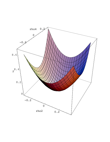
FIG. 4.: Toy model HK functional in a $\{\rho_{2},\rho_{4}\}$ frame. Note small deviations from paraboloid.

In this calculation, all coordinates $u_{\alpha}$ have been set to vanish, except $u_{2}$ and $u_{4},$ but it must be stressed that the resulting density variation, $\rho-\rho_{0},$ has non vanishing coordinates $\rho_{6},\rho_{8},...$ besides $\rho_{2}$ and $\rho_{4}.$ Such additional coordinates are small, but not very small, as shown by the grid for $\rho_{6},\rho_{8}$ in Figure 3. Qualitatively, if $u$ contains one mode $w_{\alpha}$ only, then $\rho_{\beta}$ tends to decrease when $|\alpha-\beta|$ increases. But this is likely to be valid for small enough $u$’s only, in a linear response regime. Curvature effects, evidenced by Figs. 2 and 3, must be expected further.

Of interest are plots of $F$ in $\rho$-space. If $u$ has two components $u_{2},u_{4}$ only, assume that $F$ is a function of $\rho_{2},\rho_{4}$ only. Then a gradient $\nabla F(\rho)$ can be observed directly. In Figure 4, the 3D plot of $F$ shows slight deviations from a traditional paraboloid. This is even more visible in Figure 5, showing the vector field $\{u_{2},u_{4}\}(\rho_{2},\rho_{4}),$ namely $-\nabla F.$ The field, read from Figs. 2 and 1, focuses towards the origin in $\rho$-space, but with clear distortions. We know that the field has a vanishing curl; it can be integrated back into $F.$

It is also trivial to create an approximate $F$ in the following way: i) assume indeed that $F$ depends only on $\rho_{2}$ and $\rho_{4}$ for this toy model, ii) take a few exact (numerical, actually) values of $F$ at random points taken from the partner grids shown in Figs. 1 and 2, iii) set a simple parametric ansatz such as,

$$F_{app}\simeq F_{00}+F_{10}\,\rho_{2} + F_{01}\,\rho_{4}+\left(F_{20}\,\rho_{2}^{2}+2\,F_{11}\,\rho_{2}\,\rho_{4}+F_{02}\,\rho_{4}^{2}\right)/2+\left(F_{30}\,\rho_{2}^{3}+3\,F_{21}\,\rho_{2}^{2}\,\rho_{4}+3\,F_{12}\,\rho_{2}\,\rho_{4}^{2}+F_{03}\,\rho_{4}^{3}\right)/6+$$ (66)

$$\left(F_{40}\,\rho_{2}^{4}\,+4\,F_{31}\,\rho_{2}^{3}\rho_{4}+6\,F_{22}\,\rho_{2}^{2}\,\rho_{4}^{2}+F_{13}\,\rho_{2}\,\rho_{4}^{3}+F_{04}\,\rho_{4}^{4}\right)/24\,,$$

and, finally, iv) least square fit the “exact” values selected at step ii). There are here 15 parameters and it is reasonable to select typically about twice as many exact values for the least square fit. The following result,

$$F_{app}\simeq 8.0005176-.0026263\,\rho_{2}+3.7994711\,\rho_{2}^{2}-.9776987\,\rho_{2}^{3}-.0208120\,\rho_{2}^{4}+.0034190\,\rho_{4}+$$ (67)

$$.9487531\,\rho_{2}\,\rho_{4}-.2536905\,\rho_{2}^{2}\,\rho_{4}-.5398019\,\rho_{2}^{3}\,\rho_{4}+3.7854603\,\rho_{4}^{2}+.9596720\,\rho_{2}\,\rho_{4}^{2}+$$ (68)

$$.0368183\,\rho_{2}^{2}\,\rho_{4}^{2}+.0172911\,\rho_{4}^{3}-3.0193024\,\rho_{2}\,\rho_{4}^{3}-.2356997\,\rho_{4}^{4}\,,$$ (69)

comes from fitting 26 values for $Z=4.$ Figure 6 shows several resulting contours, the smallest of which locates the minimum of $F_{app}$ very slightly only away from the origin, that is the true minimum by the very construction of the toy model. The value of the functional at the minimum turns out to be $8.0005165,$ instead of strictly $8.$ This toy numerical exercise demonstrates the possibility of contracting the description of the functional to few degrees of freedom.

FIG. 5.: Same as Fig. 4. The lines represent $-\nabla F$ at points $\{\rho_{2},\rho_{4}\}$ shown by dots. Note deviations from radial pattern.

FIG. 6.: Contours for $F_{app}.$

VI Correlations, from another toy model

In the previous sections we skirted around the difficulty of obtaining a GS with true correlations. Now we shall mix several Slater determinants, each made of $Z=4$ harmonic oscillator, one dimensional orbitals taken from $h_{0}=\frac{1}{2}(p^{2}+r^{2}).$ The Hamiltonian is a complete one,

$$H=\sum_{i=1}^{4}\left[\frac{1}{2}\left(-\frac{d^{2}}{dr_{i}^{2}}+r_{i}^{2}\right)+u_{2}\,w_{2}(r_{i})+u_{4}\,w_{4}(r_{i})\right]-V_{a}\sum_{i>j=1}^{4}\left[\delta(r_{i}-r_{j}-R_{a})+\delta(r_{i}-r_{j}+R_{a})\right].$$ (70)

This contact, finite range attraction between particles is expected to create a reasonable amount of correlations and was chosen to allow an easy precalculation and tabulation of matrix elements of $v.$ Such matrix elements are again understood to be antisymmetrized.

The first Slater determinant, $\Phi_{0},$ in the mixture contains the lowest $Z$ orbitals of the harmonic oscillator. It is expected to make the dominant component of the configuration mixture $\Psi,$ as we shall keep $u_{2},$ $u_{4}$ within the grid seen in Fig. 1, and also the strength $V_{a}$ moderate. Let $\xi_{i}$ and $\varphi_{j},$ $i,j=1,...,Z$ be the orbitals of two Slater determinants $\Xi$ and $\Phi,$ respectively. Define the cofactors $C_{ij}$ and double cofactors $C_{ikjl}$ of the determinant of scalar products $\langle\xi_{i}|\varphi_{j}\rangle.$ Such cofactors are very simple in the present orthogonal basis of orbitals, obviously. Then the matrix elements needed for the Hamiltonian matrix and the calculation of the HK functional read,

$$\langle\Xi|(H_{0}+U)|\Phi\rangle=\sum_{ik}C_{ik}\,\langle\xi_{i}|(h_{0}+u)|\varphi_{k}\rangle,\ \ \ \langle\Xi|V|\Phi\rangle=\frac{1}{4}\sum_{ijkl}C_{ikjl}\,\langle\xi_{i}\xi_{j}|v|\varphi_{k}\varphi_{l}\rangle\,.$$ (71)

With $V_{a}=5$ and $R_{a}=1$ the grids shown by Figures 7 and 8 come from a calculation with a single particle basis made of the first 10 harmonic oscillator orbitals and a corresponding Slater basis of 61 states made of $\Phi_{0}$ and all positive parity one-particle-one-hole and two-particle-two-hole determinants built upon $\Phi_{0}.$ Because of $V$ the centers of the density grids are not at the origin defined by $\Phi_{0},$ obviously. Indeed, for $u_{2}=u_{4}=0,$ this calculation gives $\{\rho_{2},\rho_{4},...\rho_{14}\}=\{-.14,-.36,-.43,-.06,.04,-.01,.005\}$ as the coordinates of the ground state density shift $\rho-\rho_{0}$ and the ground state energy is $E=-6.7,$ significantly down from $\langle\Phi_{0}|H_{0}|\Phi_{0}\rangle=8.$

FIG. 7.: Second toy model: influence of the two-body force $V$ on the $\rho_{2},\rho_{4}$ image of the grid of Fig. 1. Compare with Fig. 2.

FIG. 8.: Same as Fig. 7, but projection of the image grid into the $\rho_{6},\rho_{8}$ plane. Compare with Fig. 3.

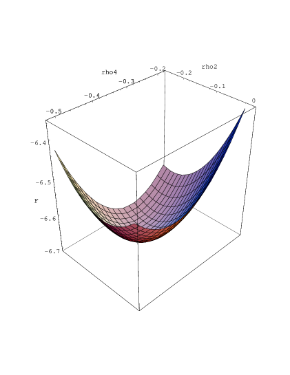
FIG. 9.: HK functional of the second toy model in $\{\rho_{2},\rho_{4}\}$ frame.

Had we taken as the origin in density space the density of the HF solution for $u=0,$ different drifts of grid centers would have been observed. Such new drifts are likely to make better signals of true correlations in $\Psi.$ For the sake of comparison between the first and the second toy models we kept $\rho_{0}$ as a reference, but we have a direct access to the amount of true correlations: it is easy here to calculate the density matrix $\hat{\rho},$ the diagonal of which gives $\rho.$ Here, for $u=0,$ the trace of $\hat{\rho}-\hat{\rho}^{2}$ is of order 5%, a reasonable amount. At that grid corner, $u_{2}=u_{4}=-2.2,$ the trace even reaches 8%. It can be concluded that this second toy model does create correlations.

While $\rho_{2}$ and $\rho_{4}$ both vary by $\sim.3$ across their grid and $\rho_{10},\rho_{12}...$ can be neglected, the variation of $\rho_{6}$ and $\rho_{8}$ across the grid is of order $\sim.1,$ which is not so small. For the sake of comparison with Fig. 4 we now show in Figure 9 a plot of the HK functional in terms of $\{\rho_{2},\rho_{4}\}$ again, but it will not be not forgotten in our agenda to find those two orthonormal combinations $\{\sigma_{2},\sigma_{4}\}$ of $\rho_{2},$ $\rho_{4},$ $\rho_{6}$ and $\rho_{8}$ which allow the “flattest” projection of the grid. It is clear that, in the spirit of Eqs. (66) and (69), the best parametrization of $F$ should now be in terms of $\{\sigma_{2},\sigma_{4}\}.$ In any case, from Fig. 9, the minimum of $F$ occurs at $\{\rho_{2},\rho_{4}\}=\{-.14,-.36\},$ the grid center, as should be. Fig. 9 also shows deviations from a paraboloid clearly stronger than those of Fig. 4.

VII Summary, discussion and conclusion

Particle number conservation is essential to that key element in the proof of the HK theorem, the one-to-one correspondence between density and external potential. However, variations of the potential should not be trivial: they should differ from constants. We treated both constraints of i) matter conservation and ii) non triviality of potential variations on the same footing: a vanishing average for both the potential and the density variations.

This constraint of vanishing average was implemented by means of a new family of orthogonal polynomials; hence appeared a set of modes in both the density and the potential spaces. We proved, numerically with toy models, that such modes might have a physical meaning, on two counts, i) converse linear responses $\delta\rho/\delta u,$ $\delta u/\delta\rho$ might be reasonably simple when described in terms of such modes, and ii) the HK functional itself might be practically truncated into projections into subspaces spanned by a few modes.

We have not discussed in this paper the constraints of positivity of the density, but it is clear that, within an algebra of polynomials such as ours, positivity conditions are not too difficult to implement. We have not discussed either more subtle constraints related to the Sobolev nature of the topological spaces available for densities. For this question, we refer to [11], [12], [13]. It can be stressed again that the compatibility of truncations of densities into a finite number of “polynomial modes” with such fine constraints can easily be tested.

An ultimate goal would be to create a constructive theory of the HK functional. The functional differential equation, $\delta F/\delta\rho=-u[\rho],$ cannot be integrated in the density space as long as $u[\rho]$ is not known accurately enough. Because of our detour through many-body perturbation theories we are clearly far from the goal, but this work gives a frame in which the task should become easier. The detour might allow a compression of the needed information through, for instance, the parametrization of a limited set of matrix elements of our matrices ${\cal D}$ for mean field approximations or $D$ in the correlated cases. Our main results are i) the existence of those special, orthogonal constrained polynomials $\Gamma_{\alpha}$ and associated modes $w_{\alpha}$ which design convenient sets of coordinates and convenient parametrizations of $F,$ $\delta F/\delta\rho,$ $\delta^{2}F/(\delta\rho\,\delta\rho^{\prime}),...$ etc., ii) the explicit relation we showed between these modes and the traditional perturbation theories used in the many-body problem and iii) the likely possibility of truncated descriptions and accurate parametrizations.

Actually, in the context of extended systems, the idea of density waves as important modes of the system has always been present. There remains to be seen, obviously, if our modes can be generalized to infinite systems. It also remains to be seen whether, for finite or infinite systems, our truncations are always justified, whether infinite resummations are possible, whether collective degrees of freedom are present, or absent, because of our new representation. Also, because of our choice of a Gaussian weight for the new family $\{\Gamma\},$ the present results are better meaningful if restricted to nuclei. A generalization to atoms and molecules obviously demands other weights for the constrained polynomials.

The usual perturbation theories have their hierarchy of modes in many-body space, most often a hierarchy of particle-hole components. Our approach, tuned to the one-body nature of the density functional, replaces the particle-holes by other modes, in a transparent way.

It is a pleasure to thank Y. Abe, R. Balian and B. Eynard for stimulating discussions.

REFERENCES

[1]
P. Hohenberg and W. Kohn, Phys. Rev. 136 3B (1964) B864.
[2] N. D. Mermin, Phys. Rev. 137 5A (1965) A1441.
[3] R. Berg and L. Wilets, Proc. Phys. Soc. A, LXVIII, (1955) 229.
[4]
W. Kohn and L. J. Sham, Phys. Rev. 140 4A (1965) A1133.
[5]
R. M. Dreizler and E. K. U. Gross, Density Functional Theory, Springer,
Berlin/Heidelberg (1990); see also the references in their review.
[6]
J.P. Perdew and S. Kurth, in A Primer in Density Functional Theory,
C. Fiolhais, F. Nogueira and M. Marques, eds., Lecture Notes in Physics,
620, Springer, Berlin (2003); see also the references in their review.
[7]
J. Dobaczewski, H. Flocard and J. Treiner, Nuclear Physics A 422 (1984)
103
[8]
G.F. Bertsch, B. Sabbey and M. Uusnäkki, Phys. Rev. C 71 (2005) 054311
[9]
J. L. Lebowitz and J.K. Percus, J. Math. Phys. 4 (1963) 116.
[10]
B. G. Giraud, M. L. Mehta and A. Weiguny, Comptes Rendus Acad. Sci 5
(2004) 871.
[11]
E.H. Lieb, Int. J. Quant. Chem. 24 (1983) 243.
[12]
H. Englisch and R. Englisch, Phys. Stat. Solidi B123 (1984) 711 and
B124 (1984) 373
[13]
R. van Leeuwen, Advances Quant. Chem. 43 (2003) 25