Self-Consistent Nuclear Shell-Model Calculation Starting from a Realistic $NN$ Potential

Abstract

First self-consistent realistic shell-model calculation for the light $p$-shell nuclei is performed, starting from the high-precision nucleon-nucleon ($NN$) CD-Bonn potential. This realistic potential is renormalized deriving a low-momentum $NN$ potential $V_{\rm low-k}$ that preserves exactly the two-nucleon low-energy physics. This $V_{\rm low-k}$ is suitable to derive a self-consistent Hartree-Fock basis that is employed to derive both effective single-particle energies and residual two-body matrix elements for the shell-model hamiltonian. Results obtained show the reliability of such a fundamental microscopic approach.

The nuclear shell model is the foundation upon which the understanding of the main features of the structure of the atomic nucleus is based. In such a frame, a central role is performed by the auxiliary one-body potential $U$, which has to be introduced in order to break up the nuclear hamiltonian as the sum of a one-body component $H_{0}$, which describes the independent motion of the nucleons, and a residual interaction $H_{1}$:

$$H=\sum_{i=1}^{A}\frac{p_{i}^{2}}{2m}+\sum_{i<j}V_{ij}=T+V=(T+U)+(V-U)=H_{0}+H_{1}~{}~{}.$$ (1)

Once $H_{0}$ has been introduced, it is possible to define a reduced Hilbert space, the model space, in terms of a finite subset of $H_{0}$’s eigenvectors. In this way the unfeasible task of diagonalizing the many-body hamiltonian (1) in a infinite Hilbert space, may be reduced to the one of solving an eigenvalue problem for an effective hamiltonian in a finite model space.

During the last forty years, a lot of efforts have been devoted to derive effective shell-model hamiltonians, starting from free nucleon-nucleon ($NN$) potentials $V_{NN}$, which reproduce with extreme accuracy the $NN$ scattering data and the deuteron properties (see for instance hjorth95 ). In particular, during the last ten years many realistic shell-model calculations have been performed to describe quantitatively with a great success the properties of nuclei over a wide mass range jiang92 ; engeland93 ; holt00 ; andreozzi97 ; coraggio99 .

In all these studies, for the sake of simplicity, a harmonic oscillator potential has been adopted as auxiliary potential. This choice simplifies the computation of the two-body interaction matrix elements, as well as the derivation of the effective hamiltonian, by way of a degenerate time-dependent pertubation theory krenc80 ; suzuki80 .

A more fundamental microscopic choice for $U$ is the Hartree-Fock (HF) potential, that is self-consistently derived from the free potential $V_{NN}$. Such a choice leads to a so-called self-consistent shell model zamick02 . It is well known, however, that modern realistic $NN$ potentials cannot be used directly to calculate a HF self-consistent potential, owing to their strong repulsion at short distances. A traditional approach to this problem is the Brueckner-Hartree-Fock (BHF) procedure, where the self-consistent potential is defined in terms of the reaction matrix vertices $G$ day67 . However, this approach cannot be considered the basis for a fully self-consistent realistic shell-model calculation zamick02 , because the choice of the BHF potential for states above the Fermi surface cannot be uniquely defined towner .

Recently, a new technique to renormalize the short-range behavior of a realistic $NN$ potential by integrating out its high-momentum components has been introduced bogner02 . The resulting low-momentum potential $V_{\rm low-k}$ is a smooth potential that preserves the low-energy physics of $V_{NN}$ and can be used directly to derive a self-consistent HF potential coraggio03 . This paves the way to perform a full self-consistent realistic shell-model calculation.

In this Letter, we present results of such a kind of shell-model calculation for light $p$-shell nuclei, starting from the high precision CD-Bonn $NN$ potential cdbonn01 .

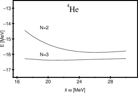
Figure 1: Behavior of $E_{\rm HF}$ with $\hbar\omega$ and $N$ for ⁴He.

First, for the sake of clarity, we outline the path through which our calculation winds up. The first step consists in deriving from the CD-Bonn potential a low-momentum potential $V_{\rm low-k}$ defined within a cutoff momentum $\Lambda$. This is done in the spirit of the renormalization group theory so obtaining a smooth potential which preserves exactly the on-shell properties of the original $V_{NN}$ bogner02 . In Ref. bogner02 a detailed discussion has been done about the value of $\Lambda$ and a criterion for its choice. According to this criterion, we have used here $\Lambda=2.1\;{\rm fm}^{-1}$. The so obtained $V_{\rm low-k}$, hermitized using the procedure based on Choleski decomposition suggested in Ref. andreozzi96 , has been used directly to solve the HF equations for ⁴He doubly closed-shell core. We remove the spurious center-of-mass kinetic energy davies71 writing the kinetic energy operator $T$ as

$$T=\frac{1}{2Am}\sum_{i<j}({\rm{\bf p}}_{i}-{\rm{\bf p}}_{j})^{2}~{}~{}.$$ (2)

So, the hamiltonian can be re-written as

$$H=\left(1-\frac{1}{A}\right)\sum_{i=1}^{A}\frac{p_{i}^{2}}{2m}+\sum_{i<j}\left(V_{ij}-\frac{{\rm{\bf p}}_{i}\cdot{\rm{\bf p}}_{j}}{mA}\right)~{}~{}.$$ (3)

The details of our HF procedure may be found in Ref. coraggio03 . In our calculations the HF single-particle (SP) states are expanded in a finite series of $N=3$ harmonic-oscillator wave-functions for ⁴He. This truncation is sufficient to ensure that the HF results do not significantly depend on the variation of the oscillator constant $\hbar\omega$, as shown in Fig. 1, where the behavior of the HF ground-state energy versus $\hbar\omega$ has been reported for different values of $N$. The value of $\hbar\omega$ adopted here is 18 MeV, as derived from the expression $\hbar\omega=45A^{-1/3}-25A^{-2/3}$ blomqvist68 .

Table 1: Experimental tilley02 and theoretical SP energies (referred to ⁴He closed-shell core) calculated including up to second- and third-order diagrams in $V_{\rm low-k}$. The experimental widths of the states are also given. Energies are in MeV.

	2nd order	3rd order	Expt.	$\Gamma$
$\pi 0p_{3/2}$	1.109	1.355	1.97	1.23
$\pi 0p_{1/2}$	4.800	4.970	3.46	6.60
$\nu 0p_{3/2}$	-0.081	0.202	0.89	0.65
$\nu 0p_{1/2}$	3.796	3.984	2.16	5.57

The HF SP eigenvectors define the basis to be used for our shell-model calculation. More precisely, we assume that doubly-magic ⁴He is an inert core and let the valence nucleons occupy the two HF orbits $0p3/2$ and $0p1/2$.

The next step is to derive the effective hamiltonian for the chosen model space. Starting from the time-dependent perturbation theory krenc80 , the effective hamiltonian is written in operator form as

$$H_{\rm eff}=\hat{Q}-\hat{Q^{\prime}}\int\hat{Q}+\hat{Q^{\prime}}\int\hat{Q}\int\hat{Q}-\hat{Q^{\prime}}\int\hat{Q}\int\hat{Q}\int\hat{Q}+~{}...~{}~{},$$ (4)

where $\hat{Q}$ is the irreducible vertex function $\hat{Q}$-box composed of irreducible valence-linked diagrams, and the integral sign represents a generalized folding operation. $\hat{Q^{\prime}}$ is obtained from $\hat{Q}$ by removing terms of first order in $V_{\rm low-k}$.

Table 2: Experimental and calculated energy levels, in MeV, in ⁶Li and ⁶He. The calculated results obtained including diagrams up to second and third order in $V_{\rm low-k}$ are compared. See text for comments.

6Li	Expt.	3rd order	2nd order
Binding energy	31.995	31.501	32.198
$E_{\rm x}(1^{+}_{1}0)$	0.0	0.0	0.0
$E_{\rm x}(3^{+}0)$	2.186	1.912	1.757
$E_{\rm x}(0^{+}1)$	3.563	2.627	2.401
$E_{\rm x}(2^{+}0)$	4.312	5.215	5.170
$E_{\rm x}(2^{+}_{1}1)$	5.366	4.911	4.590
$E_{\rm x}(1^{+}_{2}0)$	5.65	7.825	7.305
6He	Expt.	3rd order	2nd order
Binding energy	29.269	29.797	30.837
$E_{\rm x}(0^{+}_{1}1)$	0.0	0.0	0.0
$E_{\rm x}(2^{+}1)$	1.8	2.108	2.072

We take the $\hat{Q}$-box to be composed of one- and two-body diagrams through third order in $V_{\rm low-k}$.

After the $\hat{Q}$-box is calculated, the energy-independent $H_{\rm eff}$ is then obtained by summing up the folded-diagram series of Eq. (4) to all orders using the Lee-Suzuki iteration method suzuki80 . However, such a method is appropriate for degenerate model spaces only, this is the case when using a harmonic oscillator basis, as pointed out before.

Table 3: Experimental and calculated energies (MeV) and electromagnetic properties in ⁷Li. The reduced transition probabilities are expressed in W.u..

7Li	Expt.	Calc.
Binding energy	39.243	39.556
$E_{\rm x}(\frac{3}{2}^{-}_{1}\frac{1}{2})$	0.0	0.0
$E_{\rm x}(\frac{1}{2}^{-}_{1}\frac{1}{2})$	0.478	0.498
$E_{\rm x}(\frac{7}{2}^{-}_{1}\frac{1}{2})$	4.652	3.998
$E_{\rm x}(\frac{5}{2}^{-}_{1}\frac{1}{2})$	6.604	5.993
$E_{\rm x}(\frac{5}{2}^{-}_{2}\frac{1}{2})$	7.454	7.213
$E_{\rm x}(\frac{3}{2}^{-}_{2}\frac{1}{2})$	8.75	8.985
$E_{\rm x}(\frac{1}{2}^{-}_{2}\frac{1}{2})$	9.09	9.899
$E_{\rm x}(\frac{7}{2}^{-}_{2}\frac{1}{2})$	9.57	9.564
$E_{\rm x}(\frac{3}{2}^{-}_{1}\frac{3}{2})$	11.24	9.206
$Q_{\rm gs}$ [$e$ mb]	-40.6(8)	-24.4
$\mu_{\rm gs}$ [nm]	+3.256	+4.28
B(E2;$\frac{1}{2}^{-}_{1}\rightarrow\frac{3}{2}^{-}_{1}$)	19.7(1.2)	9.71
B(E2;$\frac{7}{2}^{-}_{1}\rightarrow\frac{3}{2}^{-}_{1}$)	4.2	4.18
B(M1;$\frac{1}{2}^{-}_{1}\rightarrow\frac{3}{2}^{-}_{1}$)	2.75(14)	2.37

The model space we are dealing with is non-degenerate, the unperturbed HF SP energies (respect to ⁴He closed-shell core) being 4.217 and 7.500 MeV for $\pi 0p_{3/2}$ and $\pi 0p_{1/2}$, 3.106 and 6.577 MeV for $\nu 0p_{3/2}$ and $\nu 0p_{1/2}$, respectively. So we use a generalization of the Lee-Suzuki iteration method to sum up the folded diagram series, expressed, in the case of non-degenerate model spaces, in terms of the multi-energy $\hat{Q}$-boxes kuo95 . To our knowledge this is the first time that the above technique has been employed to derive a realistic shell-model effective interaction.

As mentioned before, $H_{\rm eff}$ contains one-body contributions, the sum of all these contributions (the so-called $\hat{S}$-box shurpin83 ) is what actually determines the SP energies that should be used in a shell-model calculation. It is customary, however, to use a subtraction procedure shurpin83 so that only the two body terms of $H_{\rm eff}$ are retained and the SP energies are taken from the experimental data regarding the low lying spectra of the nuclei with one neutron or proton outside the inert core. In this calculation we have followed a more fundamental approach, where the SP energies are the theoretical ones obtained from the $\hat{S}$-box calculation (see Table I).

Table 4: Experimental and calculated electromagnetic properties in ⁶Li. The reduced transition probabilities are expressed in W.u..

6Li	Expt.	Calc.
$Q_{\rm gs}$ [$e$ mb]	-0.818(17)	-0.442
$\mu_{\rm gs}$ [nm]	+0.822	+0.866
B(E2;$3^{+}_{1}0\rightarrow 1^{+}0$)	16.5(1.3)	6.61
B(E2;$2^{+}0\rightarrow 1^{+}_{1}0$)	6.8(3.5)	6.45
B(M1;$0^{+}1\rightarrow 1^{+}_{1}0$)	8.62(18)	9.01
B(M1;$2^{+}_{1}1\rightarrow 1^{+}_{1}0$)	0.083(15)	0.154

Table 5: Same as Table IV, but for ⁷Be.

7Be	Expt.	Calc.
Binding energy	37.600	37.751
$E_{\rm x}(\frac{3}{2}^{-}_{1}\frac{1}{2})$	0.0	0.0
$E_{\rm x}(\frac{1}{2}^{-}_{1}\frac{1}{2})$	0.429	0.469
$E_{\rm x}(\frac{7}{2}^{-}_{1}\frac{1}{2})$	4.57(5)	3.922
$E_{\rm x}(\frac{5}{2}^{-}_{1}\frac{1}{2})$	6.73(10)	5.782
$E_{\rm x}(\frac{5}{2}^{-}_{2}\frac{1}{2})$	7.21(6)	7.123
$\mu_{\rm gs}$ [nm]	-1.398(15)	-1.013
B(M1;$\frac{1}{2}^{-}_{1}\rightarrow\frac{3}{2}^{-}_{1}$)	2.07(27)	1.81

In Tables II-VIII we compare experimental binding energies, low-energy spectra, and electromagnetic properties of ⁶Li, ⁶He, ⁷Li, ⁷Be, ⁸Be, ⁸Li, and ⁸B selove88 ; audi93 ; tilley02 with calculated ones. All calculations have been performed using the OXBASH shell-model code oxb . A quantitative amount of data for different nuclei is taken into account in order to verify the reliability of a self-consistent shell-model calculation. As regards binding energy results, it is well known that shell-model calculations give ground state energies referred to the closed-shell core. In our approach, we can consistently calculate the ⁴He binding energy by means of the Goldstone linked-cluster expansion coraggio03 . So, our theoretical binding energies are obtained summing the ground state energies of the open-shell nuclei to the calculated ⁴He binding energy, whose value is 25.967 MeV including up to third-order contributions. Electromagnetic properties have been calculated using effective operators krenc75 which take into account core-polarization effects.

Table 6: Experimental and calculated energies (MeV) in ⁸Be.

8Be	Expt.	Calc.
Binding energy	56.50	54.010
$E_{\rm x}(0^{+}_{1}0)$	0.0	0.0
$E_{\rm x}(2^{+}_{1}0)$	3.04	2.985
$E_{\rm x}(4^{+}_{1}0)$	11.40	10.056
$E_{\rm x}(2^{+}_{1}1)$	16.63	15.889
$E_{\rm x}(2^{+}_{2}0)$	16.92	15.174
$E_{\rm x}(1^{+}_{1}1)$	17.64	15.927
$E_{\rm x}(1^{+}_{1}0)$	18.15	15.070
$E_{\rm x}(3^{+}_{1}1)$	19.01	18.863
$E_{\rm x}(3^{+}_{1}0)$	19.24	16.983
$E_{\rm x}(4^{+}_{2}0)$	19.86	21.191

Table 7: Same as Table IV, but for ⁸Li.

8Li	Expt.	Calc.
Binding energy	41.276	44.365
$E_{\rm x}(2^{+}_{1}1)$	0.0	0.0
$E_{\rm x}(1^{+}_{1}1)$	0.981	0.922
$E_{\rm x}(3^{+}_{1}1)$	2.255	2.074
$E_{\rm x}(1^{+}_{2}1)$	3.21	4.667
$E_{\rm x}(4^{+}_{1}1)$	6.53	6.929
$E_{\rm x}(0^{+}_{1}2)$	10.822	8.230
$Q_{\rm gs}$ [$e$ mb]	24(2)	26.7
$\mu_{\rm gs}$ [nm]	+1.653	+2.89
B(M1;$1^{+}_{1}1\rightarrow 2^{+}_{1}1$)	2.8(9)	2.67
B(M1;$3^{+}_{1}1\rightarrow 2^{+}_{1}1$)	0.29(13)	0.38

In Table II we compare calculated binding energies and spectra of ⁶Li and ⁶He, obtained including contributions up to second- and third-order in perturbation theory. In all other tables calculated quantities refer to a third-order $H_{\rm eff}$.

From the inspection of Tables II-VIII, we can conclude that the overall agreement between theory and experiment may be considered to be quite satisfactory. This agreement is of the same quality, and in some cases even better, of that obtained in our previous work coraggio01 , where a realistic shell-model calculation for $p$-shell nuclei was carried out within the framework of the semi-phenomenological two-frequency shell model. It is worth to note that the inclusion of a realistic three-body force could lead to an overall improvement in the agreement with experiment, as shown in Refs. pieper01 ; navratil03

Table 8: Experimental and calculated energies (MeV) and electromagnetic properties in ⁸B.

8B	Expt.	Calc.
Binding energy	37.74	40.429
$E_{\rm x}(2^{+}_{1}1)$	0.0	0.0
$E_{\rm x}(3^{+}_{1}1)$	2.32	2.061
$E_{\rm x}(0^{+}_{1}2)$	10.619	8.245
$Q_{\rm gs}$ [$e$ mb]	64.6(1.5)	40.1
$\mu_{\rm gs}$ [nm]	+1.036	+1.73

This work was supported in part by the Italian Ministero dell’Istruzione, dell’Università e della Ricerca (MIUR).

References

- (1) M. Hjorth-Jensen, T. T. S. Kuo, and E. Osnes, Phys. Rep. 261, 125 (1995).
- (2) M. F. Jiang, R. Machleidt, D. B. Stout, and T. T. S. Kuo, Phys. Rev. C 46, 910 (1992).
- (3) T. Engeland, M. Hjorth-Jensen, A. Holt, and E. Osnes, Phys. Rev. C 48, 535(R) (1993).
- (4) A. Holt, T. Engeland, M. Hjorth-Jensen, and E. Osnes, Phys. Rev. C 61, 064318 (2000).
- (5) F. Andreozzi, L. Coraggio, A. Covello, A. Gargano, T. T. S. Kuo, and A. Porrino, Phys. Rev. C 56, R16 (1997).
- (6) L. Coraggio, A. Covello, A. Gargano, N. Itaco, and T. T. S. Kuo, Phys. Rev. C 60, 064306 (1999).
- (7) E. M. Krenciglowa and T. T. S. Kuo, Nucl. Phys. A 342, 454 (1980).
- (8) K. Suzuki and S. Y. Lee, Prog. Theor. Phys. 64, 2091 (1980).
- (9) L. Zamick, Y. Y. Sharon, S. Aroua, and M. S. Fayache, Phys. Rev. C 65, 054321 (2002).
- (10) B. D. Day, Rev. Mod. Phys. 39, 719 (1967).
- (11) I. S. Towner, A Shell Model Description of Light Nuclei (Clarendon Press, Oxford, 1977).
- (12) Scott Bogner, T. T. S. Kuo, L. Coraggio, A. Covello, and N. Itaco, Phys. Rev. C 65, 051301(R) (2002).
- (13) L. Coraggio, N. Itaco, A. Covello, A. Gargano, and T.T. S. Kuo, Phys. Rev. C 68 034320 (2003).
- (14) R. Machleidt, Phys. Rev. C 63, 024001 (2001).
- (15) F. Andreozzi, Phys. Rev. C 54, 684 (1996).
- (16) K. T. R. Davies and Richard L. Becker, Nucl. Phys. A 176, 1 (1971).
- (17) J. Blomqvist and A. Molinari, Nucl. Phys. A 106, 545 (1968).
- (18) T. T. S. Kuo, F. Krmpotić, K. Suzuki, R. Okamoto, Nucl. Phys. A 582, 205 (1995).
- (19) J. Shurpin, T. T. S. Kuo, and D. Strottman, Nucl. Phys. A 408, 310 (1983).
- (20) F. Ajzenberg-Selove, Nucl. Phys. A 490, 1 (1988).
- (21) G. Audi and A. H. Wapstra, Nucl. Phys. A 565, 1 (1993).
- (22) T. R. Tilley, C. M. Cheves, J. L. Godwin, G. M. Hale, H. M. Hoffmann, J. H. Kelley, C. G. Sheu, and H. R. Weller, Nucl. Phys. A 708, 3 (2002).
- (23) B. A. Brown, A. Etchegoyen, and W. D. M. Rae, The computer code OXBAH, MSU-NSCL, Report No. 524 (1986).
- (24) E. M. Krenciglowa and T. T. S. Kuo, Nucl. Phys. A 240, 195 (1975).
- (25) L. Coraggio, N. Itaco, A. Covello, A. Gargano, and T.T. S. Kuo, J. Phys. G 27 2351 (2001).
- (26) S. C. Pieper, V. R. Pandharipande, R. B. Wiringa, and J. Carlson, Phys. Rev. C 64, 014001 (2001).
- (27) P. Navrátil and E. W. Ormand, Phys. Rev. C 68, 034305 (2003).
- (28) P. Navrátil, J. P. Vary, W. E. Ormand, and B. R. Barrett, Phys. Rev. Lett. 87, 172502 (2001).