Self-consistent relativistic random phase approximation
with vacuum polarization

Abstract

We present a theoretical formulation for the description of nuclear excitations within the framework of relativistic random-phase approximation whereby the vacuum polarization arising from nucleon-antinucleon fields is duly accounted for. The vacuum contribution to Lagrangian is explicitly described as extra new terms of interacting mesons by means of the derivative expansion of the effective action. It is shown that the self-consistent calculation yields zero eigenvalue for the spurious isoscalar-dipole state and also conserves the vector-current density.

PACS number(s): 21.10.-k,21.60.Jz, 13.75.Cs

I Introduction

The relativistic field theory based on the quantum hadrodynamics (QHD)WA74 has been very successful in describing the nuclear properties not only for ground states but also for excited states. Although the response of a system to an external field has been already investigated in the eighties by using the relativistic random-phase approximation (RRPA) in the relativistic mean-field (RMF) basis FU85 ; KUSU85 ; IC87 ; WE87 ; HOPI88 ; FU89 ; MC89 , the self-consistent methods with nonlinear effective Lagrangian for a quantitative description of excited states have been developed only during the last few years MA97 ; CO98 ; PI00 ; RI01 ; GR03 . However, in particular, it is important to emphasize here that the negative-energy RMF states contribute essentially to the current conservation of RRPA eigenstates and the decoupling of the spurious state. In our recent study, it has been shown that the negative-energy RRPA eigenstates generated from the RRPA equation with the fully consistent basis have a significant role for gauge invariance in the electromagnetic responseHA041 .

Almost all investigations of RRPA in the QHD model referred to above, however, neglected actual antinucleon degrees of freedom. The basis set used for the RRPA calculation is usually obtained from the RMF theory wherein only positive-energy nucleons are taken into account and the Dirac sea is always regarded as unoccupied (this is sometimes called no-sea approximation). This approximation is very convenient because we do not have to puzzle over a renormalization procedure not only in the calculation of basis set under the full one-nucleon-loop contribution, which we refer to as the relativistic Hartree approximation (RHA), but also in the RRPA calculation in which the Feynman part is essentially divergent. Thus, the RRPA calculations in a finite nuclear system with the inclusion of vacuum polarization have been performed only approximately IC87 ; WE87 ; HOPI88 ; FU89 . All the RHA + RRPA calculations performed earlier have been based on the local-density approximation, that is, the renormalization of the one-nucleon loop in the RHA calculation and of the Feynman part in the polarization function were done in nuclear matter and the results were applied to finite nuclei. However, as the local-density approximation of the nucleon-antinucleon loop corrections violates the self-consistency for finite nuclei, the spurious isoscalar-dipole strength associated with the uniform translation of the center-of-mass dose not get shifted all the way down to zero excitation energyHOPI88 .

The main aim of this letter is to demonstrate as to how such a deficiency contained in the previous RHA + RRPA calculations is removed by employing the derivative-expansion method to estimate the vacuum contribution. We verify the consistency by calculating explicitly the spurious state in the isoscalar-dipole mode and the current conservation of transition densities.

In the following we work out the vacuum-polarization effects using the Lagrangian density of the Walecka $\sigma-\omega$ model which is given by

$${\cal L}_{N} = \bar{\psi}_{N}(i\gamma_{\mu}\partial^{\mu}-m_{N}+g_{\sigma}\sigma-g_{\omega}\gamma^{\mu}\omega_{\mu})\psi_{N}$$

$$+\frac{1}{2}(\partial_{\mu}\sigma)^{2}-\frac{1}{2}m_{\sigma}^{2}\sigma^{2}-U(\sigma)$$

$$-\frac{1}{4}(\partial_{\mu}\omega_{\nu}-\partial_{\nu}\omega_{\mu})^{2}+\frac{1}{2}m_{\omega}^{2}\omega_{\mu}\omega^{\mu}-\delta{\cal L},$$

where $U(\sigma)=\frac{1}{3!}g_{2}\sigma^{3}+\frac{1}{4!}g_{3}\sigma^{4}$ denotes the self-interaction terms of scalar meson, and $\delta{\cal L}=-\frac{1}{4}\zeta_{\omega}(\partial_{\mu}\omega_{\nu}-\partial_{\nu}\omega_{\mu})^{2}+\frac{1}{2}\zeta_{\sigma}(\partial_{\mu}\sigma)^{2}+\sum_{i=1}^{4}(\alpha_{i}/i!)\sigma^{i}$ represents the counterterms to regularize the nucleon self-energy. The renormalization procedure in a finite nuclear system requires considerable effort even at the mean-field levelHA042 ; ST97 . The explicit calculation of the vacuum polarization for finite system has been performed recently by Haga et. al.HA042 wherein the density variation has been found to be substantially large. The use of the effective action developed in Ref. JA74 , on the other hand, provides a direct and simple approach to estimate the vacuum corrections. It is interesting to observe that the lowest order of derivative expansion for the one-baryon-loop correction agrees with the rigorous resultsHA042 . In the derivative expansion, the contribution from the Dirac sea to the Lagrangian density, which is expressed by the trace and the logarithm of the inverse of the Dirac Green function, is expanded by derivatives of the meson fields as expressed by

$$\int\frac{d^{4}p}{(2\pi)^{4}}[Tr\ln(\gamma_{\mu}p^{\mu} - m_{N}+g_{\sigma}\sigma-g_{\omega}\gamma^{\mu}\omega_{\mu})$$

$$- Tr\ln(\gamma_{\mu}p^{\mu}-m_{N})]-\delta{\cal L}$$

$$=-V_{F}(\sigma)+\frac{1}{2}Z_{F}^{\sigma}(\sigma)( \partial_{\mu} \sigma)^{2}$$

$$+\frac{1}{4}Z_{F}^{\omega}(\sigma)( \partial_{\mu} \omega_{\nu}-\partial_{\nu}\omega_{\mu})^{2}+\cdots.$$ (2)

Each term of the right-hand side of Eq.(2) is finite, and therefore we can treat them as ordinary potential terms. Here, we may need to use a standard technique of the renormalization to obtain explicit forms of $V_{F}(\sigma)$, $Z_{F}^{\sigma}(\sigma)$, and $Z_{F}^{\omega}(\sigma)$. The method of calculating them has been discussed by many authorsAI84 ; CH85 ; OCH85 and it has also been verified that the convergence of the expansion is quite rapid within a mean-field approximationHA042 ; ST97 ; PE86 . In the present calculation, we employ only the first three terms in the right-hand side of Eq.(2).

We proceed now to describe the calculational details of the random-phase approximation based on the leading-order terms of the derivative expansion. In the $\sigma-\omega$ model, we know that the effective Lagrangian density is given by

$$\mathcal{L}^{ren}_{(1)} = \bar{\psi}_{N}^{+}(i\gamma_{\mu}\partial^{\mu}-m_{N}+g_{\sigma}\sigma-g_{\omega}\gamma^{\mu}\omega_{\mu})\psi_{N}^{+}$$

$$+\frac{1}{2}(\partial_{\mu}\sigma)^{2}-\frac{1}{2}m_{\sigma}^{2}\sigma^{2}-U(\sigma)$$

$$-\frac{1}{4}(\partial_{\mu}\omega_{\nu}-\partial_{\nu}\omega_{\mu})^{2}+\frac{1}{2}m_{\omega}^{2}(\omega_{\mu})^{2}$$

$$-V_{F}(\sigma)+\frac{1}{2}Z_{F}^{\sigma}(\sigma)(\partial_{\mu}\sigma)^{2}$$

$$+\frac{1}{4}Z_{F}^{\omega}(\sigma)(\partial_{\mu}\omega_{\nu}-\partial_{\nu}\omega_{\mu})^{2},$$

where superscript $+$ in the nucleon-field operators means that only the positive-energy states are to be treated explicitly. Then, assuming the stationary and spherical system, the ground state expectation values of the $\sigma$ and $\omega_{0}$, which are written as $\phi$ and $V_{0}$, satisfy the following coupled equations:

$$(\partial_{\mu}\partial^{\mu}+m_{\sigma}^{2})\phi =g_{\sigma}\langle\bar{\psi}^{+}\psi^{+}\rangle-U^{\prime}(\phi)-V_{F}^{\prime}(\phi)$$

$$+\frac{1}{2}Z_{F}^{\sigma\prime}(\phi)(\partial_{\mu}\phi)^{2}-\partial_{\mu}(Z_{F}^{\sigma}(\phi)\partial^{\mu}\phi)$$

$$+\frac{1}{4}{Z_{F}^{\omega}}^{\prime}(\phi)(\partial_{\mu}V_{0})^{2},$$ (4)

$$(\partial_{\mu}\partial^{\mu}+m_{\omega}^{2})V_{0} =g_{\omega}\langle\bar{\psi}^{+}\gamma^{0}\psi^{+}\rangle$$

$$+\partial_{\mu}(Z_{F}^{\omega}(\phi)\partial^{\mu}V_{0}),$$ (5)

where the contributions of the negative-energy states to source terms are contained in $V_{F}$ and $Z_{F}$. The first step in calculating the RRPA response is the computation of the RHA, which is just to solve these equations together with the Dirac equation under the potentials of $\phi$ and $V_{0}$. The potentials achieved in the mean-field calculation are then used to generate the lowest-order polarization function. We mention here that the $V_{F}$ and $Z_{F}$ terms, which appear in the meson propagator parts, correspond to the excitation of negative-energy states to all the positive-energy states. Thus, we solve the RRPA equation given by

$$\Pi_{RPA}(\Gamma^{a} ,\Gamma^{b};\mathchoice{\mbox{\boldmath$\displaystyle p$}}{\mbox{\boldmath$\textstyle p$}}{\mbox{\boldmath$\scriptstyle p$}}{\mbox{\boldmath$\scriptstyle p$}},\mathchoice{\mbox{\boldmath$\displaystyle q$}}{\mbox{\boldmath$\textstyle q$}}{\mbox{\boldmath$\scriptstyle q$}}{\mbox{\boldmath$\scriptstyle q$}};E)=\Pi_{D}(\Gamma^{a},\Gamma^{b};\mathchoice{\mbox{\boldmath$\displaystyle p$}}{\mbox{\boldmath$\textstyle p$}}{\mbox{\boldmath$\scriptstyle p$}}{\mbox{\boldmath$\scriptstyle p$}},\mathchoice{\mbox{\boldmath$\displaystyle q$}}{\mbox{\boldmath$\textstyle q$}}{\mbox{\boldmath$\scriptstyle q$}}{\mbox{\boldmath$\scriptstyle q$}};E)$$ (6)

$$+ \sum_{i}g_{i}^{2}\int d\mathchoice{\mbox{\boldmath$\displaystyle k$}}{\mbox{\boldmath$\textstyle k$}}{\mbox{\boldmath$\scriptstyle k$}}{\mbox{\boldmath$\scriptstyle k$}}_{1}d\mathchoice{\mbox{\boldmath$\displaystyle k$}}{\mbox{\boldmath$\textstyle k$}}{\mbox{\boldmath$\scriptstyle k$}}{\mbox{\boldmath$\scriptstyle k$}}_{2}\Pi_{D}(\Gamma^{a},\Gamma^{i};\mathchoice{\mbox{\boldmath$\displaystyle p$}}{\mbox{\boldmath$\textstyle p$}}{\mbox{\boldmath$\scriptstyle p$}}{\mbox{\boldmath$\scriptstyle p$}},\mathchoice{\mbox{\boldmath$\displaystyle k$}}{\mbox{\boldmath$\textstyle k$}}{\mbox{\boldmath$\scriptstyle k$}}{\mbox{\boldmath$\scriptstyle k$}}_{1};E)$$

$$\times D_{i}(\mathchoice{\mbox{\boldmath$\displaystyle k$}}{\mbox{\boldmath$\textstyle k$}}{\mbox{\boldmath$\scriptstyle k$}}{\mbox{\boldmath$\scriptstyle k$}}_{1},\mathchoice{\mbox{\boldmath$\displaystyle k$}}{\mbox{\boldmath$\textstyle k$}}{\mbox{\boldmath$\scriptstyle k$}}{\mbox{\boldmath$\scriptstyle k$}}_{2};E)\Pi_{RPA}(\Gamma^{i},\Gamma^{b};\mathchoice{\mbox{\boldmath$\displaystyle k$}}{\mbox{\boldmath$\textstyle k$}}{\mbox{\boldmath$\scriptstyle k$}}{\mbox{\boldmath$\scriptstyle k$}}_{2},\mathchoice{\mbox{\boldmath$\displaystyle q$}}{\mbox{\boldmath$\textstyle q$}}{\mbox{\boldmath$\scriptstyle q$}}{\mbox{\boldmath$\scriptstyle q$}};E),$$

where the summation is over the meson fields and $\Gamma$’s are the $4\times 4$ matrices which denote the vertex couplings. This RRPA equation exactly has the same form as that of no-sea approximation. However, it should be noted that there is an essential difference in regard to the employed meson propagator, $D_{i}$, in which we must include the vacuum-polarization corrections to perform the consistent calculation. The $\sigma-\omega$ coupling term $Z_{F}^{\omega}(\sigma)(\partial_{\mu}\omega_{\nu}-\partial_{\nu}\omega_{\mu})^{2}$ in the present Lagrangian provides the coupled equations between the $\sigma$-meson propagator and the time component of the $\omega$-meson propagator

$$\left(\begin{array}[]{cc}D_{\sigma}&D_{\sigma\omega}\\ D_{\omega\sigma}&D_{\omega 00}\\ \end{array}\right)= \left(\begin{array}[]{cc}D_{\sigma}^{0}&0\\ 0&D_{\omega 00}^{0}\\ \end{array}\right)$$ (11)

$$+\left(\begin{array}[]{cc}D_{\sigma}^{0}&0\\ 0&D_{\omega 00}^{0}\\ \end{array}\right) \left(\begin{array}[]{cc}\tilde{\Pi}_{F}^{\sigma\sigma}&\tilde{\Pi}_{F}^{\sigma\omega}\\ \tilde{\Pi}_{F}^{\omega\sigma}&\tilde{\Pi}_{F}^{\omega\omega}\\ \end{array}\right)\left(\begin{array}[]{cc}D_{\sigma}&D_{\sigma\omega}\\ D_{\omega\sigma}&D_{\omega 00}\\ \end{array}\right),$$ (18)

while the spatial component of $\omega$-meson propagator can be evaluated independently. Here, the Fourier transforms of

$$\tilde{\Pi}_{F}^{\sigma\sigma}(y,x) =\delta(x-y)\left[U^{\prime\prime}(\phi)+V_{F}^{\prime\prime}(\phi)\right.$$

$$-\frac{1}{2}Z_{F}^{\sigma\prime\prime}(\phi)(\partial_{\mu}\phi)^{2}-\frac{1}{2}Z_{F}^{\omega\prime\prime}(\phi)(\partial_{\mu}V_{0})^{2}$$

$$\left.+(\partial_{\mu}\partial^{\mu}Z^{\sigma}_{F}(\varphi))\right]+(\partial^{\mu})\left[Z_{F}^{\sigma}(\phi)\left[\partial_{\mu}\delta(x-y)\right]\right]$$ (19)

$$\tilde{\Pi}_{F}^{\sigma\omega}(y,x) =\partial_{\mu}[Z_{F}^{\omega\prime}(\phi)(\partial_{\mu}V_{0})\delta(x-y)]$$ (20)

$$\tilde{\Pi}_{F}^{\omega\sigma}(y,x) =-Z_{F}^{\omega\prime}(\phi)(\partial_{\mu}V_{0})[\partial^{\mu}\delta(x-y)]$$ (21)

$$\tilde{\Pi}_{F}^{\omega\omega}(y,x) =\partial^{\mu}\left[Z_{F}^{\sigma}(\phi)\left[\partial_{\mu}\delta(x-y)\right]\right]$$ (22)

and the effective meson propagators $D_{i}$ as well as free meson propagators $D_{i}^{0}$ are expressed as the matrices of the momentum space. Details of the formulation on the present technique along with the comparison between the Feynman part in our calculation and that in the local-density approximation will be elucidated in a forthcoming publication.

The parameter set used in the present work is listed in Table I and has been determined to reproduce the total binding energies and charge radii of the spherical nuclei in the RHA calculation. This parameter set is similar to that introduced in Ref. MA99 , where the derivative expansion has been used. Small difference between the two sets stems from the fact that in the treatment of Ref. MA99 the one-meson loop corrections have been considered in the calculation of the ground state.

Table 1: Parameter set used in the present work.

$\begin{array}[]{cccccccccc}\hline\cr\hline\cr&m_{\sigma}({\rm MeV})&m_{\omega}({\rm MeV})&\hskip 2.84526ptg_{\sigma}&\hskip 2.84526ptg_{2}({\rm fm}^{-1})&\hskip 2.84526ptg_{3}&\hskip 2.84526ptg_{\omega}\\ \hline\cr{\rm RHA}&458.0&814.0&7.10&24.09&-15.99&8.85\\ \hline\cr\hline\cr\end{array}$

In what follows we discuss the results of our RRPA calculations. In Figs. 1(a) and 1(b) we display the distributions for the Coulomb responses of isoscalar-dipole mode in ¹⁶O and ⁴⁰Ca at the momentum transfers of $q=237$ MeV and $q=118$ MeV, respectively as the function of the excitation energy. The most remarkable result of our RRPA calculations including the vacuum polarization is that the spurious state which is the collective mode corresponding to the center-of-mass motion, appears at zero excitation energy in both nuclei (shown by solid curves) as also obtained in the conventional RRPA calculation without vacuum polarization (shown by dashed curves)FU85 . The spurious state is clearly separated from the physical states, which are shown by using the small imaginary part of energy $\eta=0.05$ MeV. We emphasize that although earlier RRPA calculations with vacuum polarization have never succeeded to decouple the spurious stateHOPI88 , we are now able to achieve this by handling the Lagrangian (I) correctly.

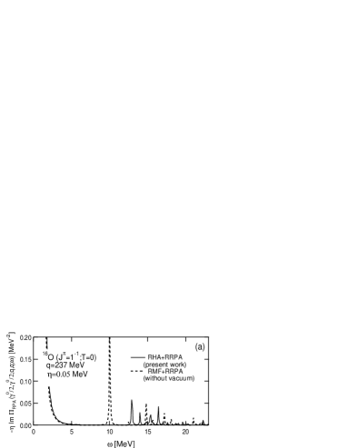
Figure 1: Distributions of isoscalar-dipole strength in (a) ¹⁶O and in (b) ⁴⁰Ca.

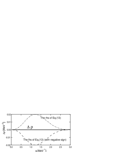
Figure 2: RHA + RRPA results for the current conservation in the transition densities for the lowest positive-energy (12.94MeV) isoscalar-dipole state in ¹⁶O. The $\Delta\varrho$ depicted by thick-solid line shows the extent of violation of current conservation. For details refer to the text.

Another important aspect for the correctness of the RPA calculations is to check whether transition charge density $\langle I^{\prime}||M_{\lambda}(q)||I\rangle$ and current density $\langle I^{\prime}||T_{\lambda L}(q)||I\rangle$, connecting the ground state $I$ and the excited states $I^{\prime}$ for different multipolarity $\lambda$ and $L$, satisfy the conservation law FU85 ; MC89 . Assuming $\omega_{N}$ denotes the excitation energy of the nucleus, the conservation relation is given by,

$$\omega_{N}\langle I^{\prime}||M_{\lambda}(q)||I\rangle =-q\sqrt{\frac{\lambda}{2\lambda+1}}\langle I^{\prime}||T_{\lambda\lambda-1}(q)||I\rangle$$

$$+ q\sqrt{\frac{\lambda+1}{2\lambda+1}}\langle I^{\prime}||T_{\lambda\lambda+1}(q)||I\rangle.$$ (23)

Our results for the RRPA transition current have been depicted in Fig. 2 where the contributions from the left-hand side (lhs) and right-hand side (rhs) of Eq. (23) are shown separately by the dashed and dash-dotted lines, respectively. Note that for the purpose of clarity the lhs of Eq. (23) has been plotted with a negative sign. The difference of these two contributions denoted by $\Delta\varrho$ and shown by thick-solid line in Fig. 2, represents the violation of the current conservation. It is gratifying to see from Fig. 2 that the RRPA transition current is sufficiently conserved.

In summary, we have studied the self-consistent RHA + RRPA method including the vacuum-polarization contribution given by the derivative-expansion method. We stress here that the present method is able to treat the change of the negative-energy states due to the presence of particles in the positive-energy states for the formation of the nucleus and also to treat consistently excited states using the RRPA. In contrast to the previous calculations based on the local-density approximation, the self-consistency of the model has been fulfilled so that we have obtained the desired results for decoupling the spurious isoscalar-dipole state, and for conserving the current density.

Also, it would be pertinent to take stock of the present scenario as regards to where we stand now. Indeed we now have a powerful method of describing the ground state of nuclei in the relativistic mean-field approximation with the inclusion of negative-energy states which are influenced by the meson mean fields. Further, we also now have a method of calculating the excited states in nuclei whereby the excitation of nucleons from negative-energy states to positive-energy states is duly included. This makes the present treatment of excited states fully consistent with the description of the ground state. Numerically, however, the $\sigma$- and $\omega$-mean fields obtained in the present treatment are found to be insufficient in strength, entailing a weaker spin-orbit splitting which is about a half as compared to that obtained in the usual RMF model SU94 . There are several possibilities to provide the missing spin-orbit splitting. One interesting idea is to explore the possibility of surface pion condensation suggested recently OG04 . Another thing could be to consider the tensor coupling for the $\omega$ meson SU942 ; MA03 . These extensions of the model constitute an effective field theory including the vacuum polarization. Further calculations testing the RRPA with these extended RHA models for a wide variety of observables in nuclear excitations would be of immense interest.

This work has been supported by MATSUO FOUNDATION, Suginami, Tokyo. We thank Prof. P. Ring and Prof. A. E. L. Dieperink for fruitful discussions.

References

• (1) J. D. Walecka, Ann. Phys. (N.Y.) 83, 491 (1974); B. D. Serot and J. D. Walecka, Adv. Nucl. Phys. 16, 1 (1986).
• (2) R. J. Furnstahl, Phys. Lett. B152, 313 (1985); J. F. Dawson and R. J. Furnstahl, Phys. Rev. C42, 2009 (1990).
• (3) H. Kurasawa and T. Suzuki, Nucl. Phys. A490, 571 (1988).
• (4) S. Ichii, W. Bentz, A. Arima, and T. Suzuki, Nucl. Phys. A487, 493 (1988).
• (5) K. Wehrberger and F. Beck, Nucl. Phys. A491, 587 (1989).
• (6) C. J. Horowitz and J. Piekarewicz, Nucl. Phys. A511, 461 (1990); J. Piekarewicz, Nucl. Phys. A511, 487 (1990).
• (7) R. J. Furnstahl and C. E. Price, Phys. Rev. C41, 1792 (1990).
• (8) J. R. Shepard, E. Rost, and J. A. McNeil, Phys. Rev. C40, 2320 (1989).
• (9) Z. Y. Ma, H. Toki, and N. Van Giai, Nucl. Phys. A627, 1 (1997); Z. Ma, A. Wandelt, N. Van Giai, D. Vretenar, P. Ring, and L. Cao Nucl. Phys. A703, 222 (2002)
• (10) C. De Conti, A. P. Galeao, and F. Krmpotic, Phys. Lett. B444, 14 (1998)
• (11) J. Piekarewicz, Phys. Rev. C64, 024307 (2001).
• (12) P. Ring, Z. Y. Ma, N. Van Giai, and D. Vretenar, Nucl. Phys. A694, 249 (2001);
• (13) V. Greco et al., Phys. Rev. C67 (2003) 015203.
• (14) A. Haga, Y. Horikawa, Y. Tanaka, and H. Toki, Phys. Rev. C69, 044308 (2004).
• (15) A. Haga, S. Tamenaga, H. Toki, and Y. Horikawa, Phys. Rev. C70, 064322 (2004).
• (16) I. W. Stewart and P. G. Blunden, Phys. Rev. D55, 3742 (1997).
• (17) R. Jackiw, Phys. Rev. D9, 1686 (1974).
• (18) I. J. R. Aitchison and C. M. Fraser, Phys. Lett. B146, 63 (1997).
• (19) L.-H. Chan, Phys. Rev. Lett. 55, 21 (1985).
• (20) O. Cheyette, Phys. Rev. Lett. 55, 2394 (1985).
• (21) R. J. Perry, Phys. Lett. B 182, 269 (1986).
• (22) G. Mao, H. StΓΆcker, and W. Greiner, Int. J. Mod. Phys. E8, 389 (1999).
• (23) R. J. Furnstahl, B. D. Serot, and H. -B. Tang, Nucl. Phys. A618, 446 (1997).
• (24) Y. Sugahara and H. Toki, Nucl. Phys. A579, 557 (1994).
• (25) Y. Ogawa, H. Toki, S. Tamenaga, H. Shen, A. Hosaka, S. Sugimoto, and K. Ikeda, Prog. Theore. Phys. 111, 75 (2004).
• (26) Y. Sugahara and H. Toki, Prog. Theor. Phys. 92, 803 (1994).
• (27) G. Mao, Phys. Rev. C67, 044318 (2003).