Quark-Hadron Duality and Parity Violating Asymmetry
of Electroweak Reactions in the $\Delta$ Region

Abstract

A dynamical modelsl1 ; sl2 ; sl3 of electroweak pion production reactions in the $\Delta$(1232) region has been extended to include the neutral current contributions for examining the local Quark-Hadron Duality in neutrino-induced reactions and for investigating how the axial $N$-$\Delta$ form factor can be determined by the parity violating asymmetry of $N(\vec{e},e^{\prime})$ reactions. We first show that the recent data of $(e,e^{\prime})$ structure functions $F_{1}$ and $F_{2}$, which exhibit the Quark-Hadron Duality, are in good agreement with our predictions. For possible future experimental tests, we then predict that the structure functions $F_{1}$, $F_{2}$, and $F_{3}$ for $(\nu,e)$ and $(\nu,\nu^{\prime})$ processes also show the similar Quark-Hadron Duality. The spin dependent structure functions $g_{1}$ and $g_{2}$ of $(e,e^{\prime})$ have also been calculated from our model. It is found that the local Quark-Hadron Duality is not seen in the calculated $g_{1}$ and $g_{2}$, while our results for $g_{1}$ and some polarization observables associated with the exclusive $p(\vec{e},e^{\prime}\pi)$ and $\vec{p}(\vec{e},e^{\prime}\pi)$ reactions are in reasonably good agreement with the recent data. In the study of parity violating asymmetry $A$ of $N(\vec{e},e^{\prime})$ reactions, the relative importance between the nonresonant mechanisms and the $\Delta$ excitation is investigated by taking into account the unitarity condition. Predictions are made for using the data of $A$ to test the axial $N$-$\Delta$ form factors determined previously in the studies of $N(\nu_{\mu},\mu^{-}\pi)$ reactions. The predicted asymmetry $A$ are also compared with the Parton Model predictions for future experimental investigations of Quark-Hadron Duality.

I Introduction

In recent years, a dynamical model had been developedsl1 ; sl2 to investigate electromagnetic pion production reactions in the region near the $\Delta$(1232) resonance. The model was subsequently extendedsl3 to also investigate neutrino-induced reactions $(\nu_{\mu},\mu^{-}\pi)$. Fairly consistent descriptions of all of the available data in the $\Delta$ region have been obtained. In this work, we further extend this model (called the SL model ) to address two questions of current interest : (1) Will Hadron-Quark Duality first observed by Bloom and Gilmanbg in inclusive $p(e,e^{\prime})$ be also seen in the neutrino-induced $N(\nu,e)$ and $N(\nu,\nu^{\prime})$ reactions ? (2) How can parity violating asymmetry of inclusive $N(\vec{e},e)$ reaction be used to improve our knowledge about the axial $N$-$\Delta$ form factor ? Experimental data for testing our predictions can be obtained at new neutrino facilitiesfermi and Jefferson Laboratory (JLab)well ; bosted .

Our first step is to construct neutral currents within the SL model. This then allows us to extend our previous calculationssl3 of $N(\nu_{\mu},\mu^{-}\pi)$ reactions to also predict $N(\nu,\nu^{\prime}\pi)$ reactions for examining some questions concerning the Quark-Hadron Duality. Simply speaking, an inclusive lepton scattering observable exhibits Quark-Hadron Duality when an average of this quantity over an appropriately chosen scaling variable in the resonance region is close to that in the Deeply Inelastic Scattering (DIS) region. More details on this subject can be found in a recent review by Melnitchouk, Ent and Keppelmeln . The Quark-Hadron Duality was first observedbg for the $p(e,e^{\prime})$ structure function $F_{2}=\omega W_{2}$. Recent experimental datanicu ; liang for both $F_{2}$ and $F_{1}=m_{N}W_{1}$ have further confirmed more quantitatively this interesting observation. Theoretical attempts in understanding the Quark-Hadron Duality within QCD were already madenach ; gp ; rgp in 1970’s. More recent works are reported in, for example, Refs.xi1 ; xi2 ; mueller ; carlson ; edel ; meln-1 . Within the Standard modelholstein , it is natural to ask whether the Quark-Hadron Duality should also exist in the neutrino-induced $N(\nu,e)$ and $N(\nu,\nu^{\prime})$ reactions (from nowon, $\nu$ and $e$ denote the neutrinos and charged leptons, respectively, of any generation within the Standard Model). In the absence of necessary neutrino data, this can be explored theoretically in the $\Delta$ region using the extended SL model presented in this paper. Obviously, we can only explore the ’local’ Quark-Hadron Duality in the $\Delta$ region.

We will also report on our investigations of the spin dependent structure functions $g_{1}$ and $g_{2}$ of $(e,e^{\prime})$ processes. To see the accuracy of our model in predicting these quantities, we first show that some recent databiselli ; joo of the polarization observables associated with the exclusive $p(\vec{e},e^{\prime}\pi)$ and $\vec{p}(\vec{e},e^{\prime}\pi)$ reactions agree well with the predictions from the considered SL model. We then find that $g_{1}$ calculated from our model agree reasonably well with the recent datafatemi , but do not show Quark-Hadron Duality when compared with the DIS dataabe . The calculated $g_{2}$ is also found to be rather different from the DIS data which can be described reasonably well by the Wandzura-Wilczek formulawwil .

Our second task in this work is to apply the extended SL model to address some questions concerning the $N$-$\Delta$ form factors. It has been well recognized that these form factors are important information for testing current hadron models and also lattice QCD calculations in the near future. The vector parts of the $N$-$\Delta$ form factors in the $Q^{2}\leq 4$ (GeV/c)² region have been rather well determined by analyzing very extensive high precision data of electromagnetic pion production reactions, as reviewed in Ref.burkertlee . On the other hand, the axial vector $N$-$\Delta$ form factor is not well determined mainly because of the short of high precision data of neutrino-induced pion production reactions in the $\Delta$ region. For example, the axial $N$-$\Delta$ from factor determined in Ref.sl3 is rather different from the one determined previouslykitagaki . This leads to uncertainties in interpreting the axial $N$-$\Delta$ form factor in terms of the hadron structure calculations such as those reported in Refs.nimi-1 ; nimi-2 ; golli ; bruno . The situation will be improved when the data from new neutrino facilities become available in the near future. Alternatively, progress can be made by following Refs.cg ; jones ; isha ; hwang ; nath ; musolf ; hammer ; nimi-3 ; rekalo to investigate the parity violating asymmetry of inclusive $N(\vec{e},e^{\prime})$ reactions. This polarization observable is due to the interference between the electromagnetic currents and neutral currents and hence can be used to explore the axial $N$-$\Delta$ form factor. Experimental effort in this direction is being madewell at JLab. To facilitate this study, we have applied the extended SL model to explore the dependence of the parity violating asymmetry of $N(\vec{e},e^{\prime})$ on the axial $N$-$\Delta$ form factor.

In section II, we will specify the considered models of electromagnetic currents ($em$), weak charged currents ($cc$), and weak neutral currents ($nc$). We first recall their forms in the Standard modelholstein and then specify how such currents are defined in terms of hadronic degrees of freedom of the SL model. In section III, we give expressions of the inclusive cross sections and indicate how the structure functions are calculated within our hadronic model and Parton Model. Section IV is devoted to present results for studying the Quark-Hadron Duality in the $\Delta$ region. The predicted $N(e,e^{\prime})$ structure functions will also be compared with the recent data. The results for the parity violating asymmetry of the inclusive $N(\vec{e},e^{\prime})$ will be given in section V. A summary is given in section VI.

II Models of Electroweak Currents

We first recall the electroweak currents defined in the Standard Modelholstein . In the considered $\Delta$ excitation region, we can eliminate heavy $W$ and $Z$ bosons and keep interactions involving only up ($u$) and down ($d$) quarks. The interaction Lagrangian for our study can then be written as

$$L_{eff} = -\sqrt{4\pi\alpha}[\bar{e}\gamma^{\mu}e+j^{\mu}_{em}]A_{\mu}$$ (1)

$$-\frac{G_{F}V_{ud}}{\sqrt{2}}[\bar{\nu}\gamma_{\mu}(1-\gamma_{5})ej^{\mu\dagger}_{cc}+\bar{e}\gamma_{\mu}(1-\gamma_{5})\nu j^{\mu}_{cc}]$$

$$-\frac{G_{F}}{\sqrt{2}}[\bar{\nu}\gamma_{\mu}(1-\gamma_{5})\nu+\bar{e}(2g_{V}^{e}\gamma_{\mu}-2g_{A}^{e}\gamma_{\mu}\gamma^{5})e]j^{\mu}_{nc}\,,$$

where $\alpha=1/137$, $G_{F}=1.1664\times 10^{-5}$ GeV^-2, $g_{V}^{e}=-1/2+2\sin^{2}\theta_{W}$, $g_{A}^{e}=-1/2$, $A_{\mu}$ is the photon field, $e$ and $\nu$ are the field operators of the charged leptons and neutrinos, respectively. The Weinberg angle $\theta_{W}$ is known empirically to be $\sin^{2}\theta_{W}=0.231$ and $V_{ud}=0.974$ is the the Cabibbo-Kobayashi-Maskawa (CKM) coefficient. The electromagnetic current ($j^{\mu}_{em}$), weak charge current ($j^{\mu}_{cc}$) and weak neutral current ($j^{\mu}_{nc}$) carried by $u$ and $d$ quarks can be written as

$$j^{\mu}_{em} = \frac{2}{3}\bar{u}\gamma^{\mu}u-\frac{1}{3}\bar{d}\gamma^{\mu}d\,,$$ (2)

$$j^{\mu}_{cc} = \bar{u}\gamma^{\mu}(1-\gamma_{5})d\,,$$ (3)

$$j^{\mu}_{nc} = \frac{1}{2}[\bar{u}\gamma^{\mu}(1-\gamma_{5})u-\bar{d}\gamma^{\mu}(1-\gamma_{5})d]-2\sin^{2}\theta_{W}j_{em}^{\mu}\,.$$ (4)

With the simplification that only $u$ and $d$ quarks are kept, it is well knownmusolf that the above currents can be classified according ’strong’ isospin. We thus can write

$$j^{\mu}_{em} = V^{\mu}_{3}+V^{\mu}_{isoscalar}\,,$$ (5)

$$j^{\mu}_{cc} = (V^{\mu}_{1}+iV^{\mu}_{2})-(A^{\mu}_{1}+iA^{\mu}_{2})\,,$$ (6)

$$j^{\mu\dagger}_{cc} = (V^{\mu}_{1}-iV^{\mu}_{2})-(A^{\mu}_{1}-iA^{\mu}_{2})\,,$$ (7)

$$j^{\mu}_{nc} = (1-2\sin^{2}\theta_{W})j^{\mu}_{em}-V^{\mu}_{isoscalar}-A^{\mu}_{3}\,,$$ (8)

where the isospin components of the vector ($V$) and axial vector ($A$) currents are defined as

$$V^{\mu}_{i} = \bar{q}\gamma^{\mu}\frac{\tau_{i}}{2}q\,,$$ (9)

$$A^{\mu}_{i} = \bar{q}\gamma^{\mu}\gamma_{5}\frac{\tau_{i}}{2}q\,,$$ (10)

$$V^{\mu}_{isoscalar} = \bar{q}\frac{1}{6}\gamma^{\mu}q\,.$$ (11)

Here we have defined an isospin doublet field operator $\bar{q}=q^{+}\gamma^{0}=(u^{+},d^{+})\gamma^{0}$ and $\tau_{i}$ is the usual Pauli operator.

The above expressions will allow us to calculate electroweak structure functions of deeply inelastic $(e,e^{\prime})$, $(\nu,e)$ and $(\nu,\nu^{\prime})$ processes within the Parton Model, as explained in, for example, Ref.tw . However, they can not be used directly for investigating meson production reactions in the resonance region where the perturbative QCD is not applicable. At the present time, the most tractable ways for investigating these reactions are in terms of hadronic degrees of freedom. The starting point is a hadronic effective Lagrangian constrained by the symmetry properties of the Standard Model. Accordingly, the resulting electroweak currents have the forms of Eqs.(5)-(8), but are written in terms of hadronic field operators. This can be achieved by using the standard effective chiral lagrangian methodspark ; gl ; holstein . In the SL model developed in Refs.sl1 ; sl2 ; sl3 , the constructed electroweak currents are expressed in terms of the field operators of the nucleon ($N$), Delta ($\Delta$), pion ($\vec{\pi}$), omega meson ($\omega$), and rho meson ($\vec{\rho}$). They can be written as

$$\vec{V}^{\mu}\cdot\vec{v}_{\mu} = \bar{N}{}[\gamma^{\mu}\vec{v}_{\mu}-\frac{\kappa^{V}}{2m_{N}}\sigma^{\mu\nu}\partial_{\nu}\vec{v}_{\mu}]\cdot\frac{\vec{\tau}}{2}N+\frac{g_{A}}{2F}\bar{N}\gamma^{\mu}\gamma_{5}[\vec{v}_{\mu}\cdot\vec{\tau}]N\times\vec{\pi}$$ (12)

$$+[\vec{\pi}\times\partial^{\mu}\vec{\pi}]\cdot\vec{v}_{\mu}-\frac{g_{\omega\pi V}}{m_{\pi}}\epsilon_{\alpha\mu\nu\delta}[\partial^{\alpha}\vec{v}^{\mu}]\cdot\vec{\pi}[\partial^{\nu}\omega^{\delta}]-i\bar{\Delta}_{\mu}\vec{T}\cdot\vec{v}_{\nu}\Gamma^{\mu\nu}_{V}N\,,$$

$$\vec{A}^{\mu}\cdot\vec{v}_{\mu} = g_{A}\bar{N}\gamma^{\mu}\gamma_{5}\frac{\vec{\tau}}{2}\cdot\vec{v}_{\mu}N-F\partial^{\mu}\vec{\pi}\cdot\vec{v}_{\mu}-f_{\rho\pi A}(\vec{\rho}^{\mu}\times\vec{\pi})\cdot\vec{v}_{\mu}+\bar{\Delta}_{\nu}\vec{T}\cdot\vec{v}_{\mu}\Gamma^{\mu\nu}_{A}N\,,$$ (13)

where $\vec{v}_{\mu}$ is an arbitrary isovector function, $F=93$ MeV is the pion decay constant, and $g_{A}=1.26$ is the axial coupling strength of the nucleon. The other parameters as well as the vertex $\Gamma^{\mu\nu}_{A,V}$ and isospin operator $T$ of the $N$-$\Delta$ transition are given in Refs.sl1 ; sl2 ; sl3 . With the electromagnetic current $j^{\mu}_{em}$ given explicitly in Ref.sl1 , the relation Eq.(5) and Eq.(12) can be used to get $V^{\mu}_{isoscalar}$ and hence $j^{\mu}_{nc}$ of Eq.(8) is also completely determined within the SL model. The neutral current $j^{\mu}_{nc}$ is needed to extend the calculations of Refs.sl1 ; sl2 ; sl3 to also study $(\nu,\nu^{\prime}\pi)$ reactions and the parity violating asymmetry of the $(\vec{e},e^{\prime})$ reaction.

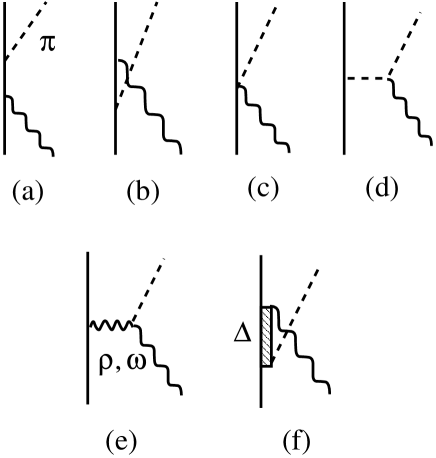
Figure 1: Non-resonant pion production mechanisms of the SL model. See text for explaining how these mechanisms are related to the electrmagnetic current, charged current, and neutral current.

The electroweak currents defined by Eqs.(5)-(8) and (12)-(13) must be supplemented by additional effective Lagrangians describing the haronic interactions, such as $\pi NN$, $\pi N\Delta$, $\rho NN$, $\rho\pi\pi$, and $\omega NN$ couplings, to calculate the meson production amplitudes within the SL model. The details of such a dynamical approach have been given in Refs.sl1 ; sl2 ; sl3 . Here it is sufficient to just illustrate schematically the basic meson production mechanisms of the SL model. In Fig.1, we show the constructed non-resonant pion production mechanisms. For the $em$ current contributions, the waved-line is photon and all diagrams contribute. For $cc$ and $nc$ current contributions, the wave-line is the vector current $V$ or axial vector current $A$. Like the $em$ case, all terms in Fig.1 contribute to $nc$ amplitude but with different isospin weighting factors defined by Eqs.(5) and (8). For the $cc$ contributions, all terms contribute to the amplitudes induced by the vector current $V$ except that the $\rho$ exchange in (c) should be excluded because it is an isoscalar interaction. The $cc$’s amplitude due to axial vector current $A$ contains only mechanisms (a), (b), (e) with only $\rho$ exchange, and (f). In both $cc$ and $nc$ cases, the pion pole term due to the second term $-F\partial^{\mu}\vec{\pi}\cdot\vec{v}_{\mu}$ of axial current Eq.(13) has additional contributions, as explained in Ref.sl3 .

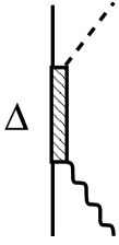
Figure 2: The $\Delta$ excitation mechanism.

The $\Delta$ excitation mechanism is illustrated in Fig.2. For the later discussions in this paper, here we recall that the matrix element of the axial $N$-$\Delta$ coupling $\Gamma_{A}^{\mu\nu}$ in Eq.(13) can be written as

$$<p_{\Delta}\mid\Gamma^{\mu\nu}_{A}\mid p_{N}> = d_{1}(q^{2})g^{\mu\nu}+\frac{d_{2}(q^{2})}{m^{2}_{N}}P_{\alpha}(q^{\alpha}g^{\mu\nu}-g^{\alpha\mu}q^{\nu})$$ (14)

$$-\frac{d_{3}(q^{2})}{m^{2}_{N}}q^{\mu}p_{N}^{\nu}-i\frac{d_{4}(q^{2})}{m^{2}_{N}}\epsilon^{\mu\nu\alpha\beta}P_{\alpha}q_{\beta}\gamma_{5}\,,$$

where $p_{\Delta}$ and $p_{N}$ are the momenta of the $\Delta$ and $N$, respectively, $q=p_{\Delta}-p_{N}$, and $P=(p_{\Delta}+p_{N})$. The strengths of the form factors at $Q^{2}=-q^{2}=0$ are identified with the quark model predictionsnimi-1 and are found to be $d_{i}(0)=D_{i}\frac{6}{\sqrt{2}5}g_{A}$ with $g_{A}=1.26$, $D_{1}=0.969$, $D_{2}=-0.180$, $D_{3}=0.836$, and $d_{4}=0$. In Ref.sl3 , it was found that all of the available data of $N(\nu_{\mu},\mu^{-}\pi)$ data in the $\Delta$ region can be well described if the $q^{2}$-dependence of each form factor in Eq.(14) is taken to be ($Q^{2}=-q^{2}$)

$$d_{1,2}(Q^{2}) = d_{1,2}(0)G^{A}_{N,\Delta}(Q^{2})\,,$$

$$d_{3}(Q^{2}) = d_{3}(0)\frac{m_{N}^{2}}{Q^{2}+m_{\pi}^{2}}G^{A}_{N,\Delta}(Q^{2})\,,$$

with

$$G^{A}_{N,\Delta}(Q^{2})=(1+aQ^{2})exp(-bQ^{2})G_{A}(Q^{2})\,,$$ (15)

where $a=0.154$ (GeV/c)^-2, $b=0.166$ (GeV/c)², and $G_{A}(Q^{2})=1/(1+Q^{2}/M^{2}_{A})^{2}$ with $M_{A}=1.02$ GeV is the nucleon axial form factormiss . The corresponding vector form factor $G^{V}_{\Delta,N}(Q^{2})$, which is associated with $\Gamma^{\mu\nu}_{V}$ of Eq.(12) and has been well determinedsl1 ; sl2 by analyzing the data of pion electroproduction, has the same form as Eq.(15) except that $G_{A}(Q^{2})$ is replaced by the usual proton form factor $G_{p}(Q^{2})=1/(1+Q^{2}/\Lambda_{p}^{2})^{2}$ with $\Lambda_{p}^{2}=0.71$ (GeV/c)².

We further mention that the electroweak pion production amplitudes (denoted as $J$ from nowon) calculated within the SL model can be written schematically in the center of mass (c.m.) frame of the final $\pi N$ system as

$$J_{\pi N,aN}(k,q,W)=J_{\pi N,aN}^{(n.r.)}(k,q,W)+\frac{\bar{\Gamma}^{\dagger}_{\Delta,\pi N}(k,W)\bar{\Gamma}_{\Delta,aN}(q,W)}{W-m_{\Delta}-\Sigma(W)}\,,$$ (16)

where $a=\gamma$, W or $Z$ bosons, $q$ and $k$ are the relevant initial and final momenta, $\Sigma(W)$ is the $\Delta$ self-energy. The non-resonant amplitudes $J^{(n.r.)}_{\pi N,aN}(k,q,W)$ are calculated from

$$J^{(n.r.)}_{\pi N,aN}(k,q,W)=v_{\pi N,aN}+t_{\pi N,\pi N}G_{\pi N}(W)v_{\pi N,aN}\,,$$ (17)

where $v_{\pi N,aN}$ are the non-resonant amplitudes illustrated in Fig.1, $t_{\pi N,\pi N}$ is the non-resonant $\pi N$ scattering amplitude, and $G_{\pi N}(W)$ is the $\pi N$ propagator. Note that the second term of Eq.(17) is the consequence of the unitarity condition. This is neglected in the previous investigationshwang ; hammer ; nimi-3 ; rekalo of the effects due to the non-resonant amplitudes on the parity violating asymmetry of $N(\vec{e},e^{\prime})$ reaction. Furthermore, the non-resonant mechanisms considered in those works also differ from what are illustrated in Fig.1 and well tested in extensive investigations of exclusive $N(\gamma,\pi)$, $N(e,e^{\prime}\pi)$, and $N(\nu_{\mu},\mu^{-}\pi)$ reactions. For example, the vector meson exchanges are not included in Refs.hammer ; nimi-3 and pseudo-scalar $\pi NN$ coupling, instead of the pseudo-vector coupling used in the SL model, is used in Ref.rekalo .

The resonant term in Eq.(16) is defined by the dressed vertices which contain the influence of the non-resonant interactions as given by the following equation

$$\bar{\Gamma}_{\Delta,aN}(q,W) = \Gamma_{\Delta,aN}(q)+\int d{\bf k}\Gamma_{\Delta,\pi N}(k)G_{\pi N}(k,W)J_{\pi N,aN}^{(n.r.)}(k,q,W)\,,$$ (18)

where $\Gamma_{\Delta,aN}(q)$ is the $bare$ $N$-$\Delta$ form factor. The second term in Eq.(18) is commonly called the meson cloud contributions to the $N$-$\Delta$ transition. Explicit calculations of these meson cloud effects also mark an important difference between this work and all of the previous investigationscg ; jones ; isha ; hwang ; nath ; musolf ; hammer ; nimi-3 ; rekalo of parity violating asymmetry of $N(\vec{e},e^{\prime})$ reactions. We emphasize that Eqs.(16)-(18) satisfy the unitarity condition which is essential in interpreting the meson production data, as explained in Refs.sl1 ; sl2 ; sl3 as well as in many works reviewed in Ref.burkertlee .

III Calculations of Structure Functions

With the Lagrangian Eq.(1), the formula for calculating the exclusive cross sections for $(e,e^{\prime}\pi)$ and $(\nu,e\pi)$ processes are given in details in Refs.sl1 ; sl2 ; sl3 . The formula for calculating $(\nu,\nu^{\prime}\pi)$ cross sections can be easily obtained from Ref.sl3 with minor modifications. In this paper, we focus on inclusive processes. Their cross sections can be more simply written in terms of structure functions.

Following Ref.tw , the symmetry properties require that the lepton scattering structure functions $W_{1}$, $W_{2}$ and $W_{3}$ are in general related to the hadron tensor $W^{\mu\nu}$ by

$$W^{\mu\nu} = -W_{1}g^{\mu\nu}+\frac{W_{2}}{m_{N}^{2}}p^{\mu}p^{\nu}+i\frac{W_{3}}{2m_{N}^{2}}\epsilon^{\mu\nu\alpha\beta}p_{\alpha}q_{\beta}\,,$$ (19)

where the convention $\epsilon^{0123}=-1$ is chosen. The structure functions are functions of two independent invariant variables. One usually chooses $Q^{2}$ and the invariant mass $W=\sqrt{s}=\sqrt{(p+q)^{2}}$ in the resonance region, but chooses Bjorken scaling variable $x=Q^{2}/(2p\cdot q)$ and $Q^{2}$ in the deeply inelastic region. Here $q$ and $p$ are the momenta of the exchanged boson ($\gamma$, $W$ or $Z$) and the initial nucleon, respectively. The unpolarized inclusive $N(e,e^{\prime})$ cross sections can then be written as

$$\frac{d\sigma}{d\Omega dE^{\prime}}=\frac{4\alpha^{2}E^{\prime 2}}{Q^{4}}[2W_{1}\sin^{2}\frac{\theta}{2}+W_{2}\cos^{2}\frac{\theta}{2}]\,,$$ (20)

with

$$Q^{2}=-q^{2}=4EE^{\prime}\sin^{2}\frac{\theta}{2}\,,$$ (21)

where $E$ and $E^{\prime}$ are the incident and outgoing lepton energies, respectively, $\theta$ is the lepton scattering angle with respect to the incident lepton . For inclusive $(\nu,e^{-})$ and $(\bar{\nu},e^{+})$ processes, we have

$$\frac{d\sigma^{\nu,\bar{\nu}}}{dE^{\prime}d\Omega^{\prime}}=\frac{G^{2}_{F}\mid V_{ud}\mid^{2}}{2\pi^{2}}E^{\prime 2}[2W_{1}\sin^{2}\frac{\theta}{2}+W_{2}\cos^{2}\frac{\theta}{2}\pm W_{3}\frac{E+E^{\prime}}{m_{N}}\sin^{2}\frac{\theta}{2}]\,,$$ (22)

where the sign in front of $W_{3}$ is $+$ (-) for $(\nu,e^{-})$ ($(\bar{\nu},e^{+})$). For $(\nu,\nu^{\prime})$, the cross section formula is the same as Eq.(22) except that the factor $\mid V_{ud}\mid^{2}$ is removed.

Within the hadronic models, such as the SL model considered in this paper, the hadron tensor $W^{\mu\nu}$ in the region near the $\Delta$ excitation can be calculated from summing all contributions from $a(q)+N(p)\rightarrow\pi(k)+N(p)$ with $a=\gamma,W,Z$. We can write in general the hadron tensor $W^{\mu\nu}$ for electroweak pion reactions as

$$W^{\mu\nu} = \sum<f|J_{\alpha}^{\mu}|i>^{*}<f|J_{\alpha}^{\nu}|i>\,,$$ (23)

where $\alpha=em,cc,nc$ denotes the considered current, and we have introduced concise notations

$$\sum=\sum_{\bar{i}}\sum_{f}(2\pi)^{3}\delta^{4}(p+q-p^{\prime}-k)\frac{E_{N}}{m_{N}}\,,$$ (24)

and

$$<f\mid J_{\alpha}^{\mu}\mid i> = \frac{1}{(2\pi)^{3}}\sqrt{\frac{m_{N}^{2}}{E_{N}E_{N}^{\prime}2E_{\pi}}}<k(t_{\pi}),p^{\prime}(s^{\prime},t^{\prime})|J_{\alpha}^{\mu}(q)|p(s,t)>\,,$$ (25)

Here $(s,t)$ denote the z-components of the nucleon spin-isospin, $t_{\pi}$ the z-component of the pion isospin, and $<k(t_{\pi}),p^{\prime}(s^{\prime},t^{\prime})|J_{\alpha}^{\mu}(q)|p(s,t)>$ is the $a+N\rightarrow\pi+N$ amplitude with $a=\gamma$, $W$, $Z$ for $\alpha=em$, $cc$, and $nc$, respectively. In the dynamical approach of Refs.sl1 ; sl2 ; sl3 , the current matrix element Eq.(25) has the form of Eq.(16), consisting of a non-resonant term and a resonant term.

From Eqs.(19) and (23), one can derive the expressions for calculating the structure functions $W_{1}$, $W_{2}$, and $W_{3}$ from the current matrix elements defined by Eq.(25). It is convenient to calculate these structure functions in the center of mass (c.m.) frame of the initial $aN$ and final $\pi N$ systems. The direction of the momentum-transfer is chosen to be the quantization $z$-direction : i.e. $q=(\omega_{c},0,0,\mid{\bf q}_{c}\mid)$ for the exchanged boson and $p=(E_{N},0,0,-\mid{\bf q}_{c}\mid)$ for the initial nucleon. We then have for the contribution from current $j_{\alpha}$ with $\alpha=em,cc,nc$,

$$W_{1} = \frac{1}{2}\sum[|<f\mid J_{\alpha}^{x}\mid i>|^{2}+|<f\mid J_{\alpha}^{y}\mid i>|^{2}]\,,$$ (26)

$$W_{2} = \frac{Q^{2}}{{\bf q}^{2}}\sum[\frac{1}{2}(|<f\mid J_{\alpha}^{x}\mid i>|^{2}+|<f\mid J_{\alpha}^{y}\mid i>|^{2})+\frac{Q^{2}}{{\bf q}_{c}^{2}}|<f\mid\bar{J}_{\alpha}\mid i>|^{2}]\,,$$ (27)

$$W_{3} = -\frac{2m_{N}}{\mid{\bf q}\mid}\sum Im[<f\mid J_{\alpha}^{x}\mid i><f\mid J_{\alpha}^{y}\mid i>^{*}]\,,$$ (28)

where $\bar{J}_{\alpha}=J_{\alpha}^{0}+\frac{\omega_{c}}{Q^{2}}J_{\alpha}\cdot q$, and ${\bf q}$ is three-momentum transfer in the laboratory frame (i.e. $q=(\omega,{\bf q})$). In practice, the calculation of any term of the structure functions defined by Eqs.(26)-(28) can be obtained from appropriate combinations of the following integrations

$$I^{\mu\nu}_{\alpha,\beta} = \sum[<f\mid J_{\alpha}^{\mu}\mid i><f\mid J_{\beta}^{\nu}\mid i>^{*}]$$

$$= \frac{1}{2}\sum_{s,s^{\prime},t^{\prime},t_{\pi}}\int d\Omega_{\pi}\frac{|{\bf k}_{c}|m_{N}}{16\pi^{3}W}<k(t_{\pi})p^{\prime}(s^{\prime},t^{\prime})|J_{\alpha}^{\mu}(q)|p(s,t)><k(t_{\pi})p^{\prime}(s^{\prime},t^{\prime})|J_{\beta}^{\nu}(q)|p(s,t)>^{*}\,.$$

were $\alpha,\beta=em,cc,nc$, and ${\bf k}_{c}$ is final pion momentum in the final $\pi N$ c.m. system.

We will also examine the spin dependent structure functions of $(e,e^{\prime})$. They are definedtw by writing the hadron tensor for a polarized target with spin vector $S^{\mu}$ ($S^{2}=-1,p\cdot S=0$) as

$$W^{\mu\nu}=W^{\mu\nu}_{S}+W^{\mu\nu}_{A}\,,$$ (30)

where

$$W^{\mu\nu}_{S} = W_{1}(-g^{\mu\nu}+\frac{q^{\mu}q^{\nu}}{q^{2}})+\frac{W_{2}}{M^{2}}(p^{\mu}-\frac{p\cdot q}{q^{2}}q^{\mu})(p^{\nu}-\frac{p\cdot q}{q^{2}}q^{\nu})\,,$$ (31)

$$W^{\mu\nu}_{A} = i\frac{\epsilon^{\mu\nu\alpha\beta}q_{\alpha}}{p\cdot q}[g_{1}S_{\beta}+g_{2}(S_{\beta}-\frac{S\cdot q}{p\cdot q}p_{\beta})]\,.$$ (32)

With some derivations, one can show that

$$g_{1} = \frac{1}{1+\frac{Q^{2}}{\omega^{2}}}[\frac{Q^{2}}{\omega^{2}}X^{y0}+X^{xy}]\,,$$ (33)

$$g_{2} = \frac{1}{1+\frac{Q^{2}}{\omega^{2}}}[X^{y0}-X^{xy}]\,,$$ (34)

with

$$X^{y0} = -m_{N}\frac{\omega}{\mid{\bf q}\mid}Im[I^{y0}_{em,em}\mid_{s=S(x)}]\,,$$ (35)

$$X^{xy} = -m_{N}Im[I^{xy}_{em,em}\mid_{s=S(z)}]\,,$$ (36)

where $I^{\mu\nu}_{em,em}\mid_{s=S(i)}$ is the same as that defined in Eq.(29) except that the initial nucleon projection $s$ is not summed over but is fixed in the chosen direction defined by $S(i)$. $S(x)$ ($S(z)$) means that the initial nucleon spin is polarized in the direction perpendicular (parallel) to the incident electron direction.

For investigating Quark-Hadron Duality, we would like to compare the structure functions calculated from using the above formula for hadronic models with those calculated from the quark currents Eqs.(2)-(4) in the deeply inelastic region. With the standard definitions

$$F_{1}(x,Q^{2}) = m_{N}W_{1}(x,Q^{2})\,,$$

$$F_{2}(x,Q^{2}) = \omega W_{2}(x,Q^{2})\,,$$

$$F_{3}(x,Q^{2}) = \omega W_{3}(x,Q^{2})\,,$$ (37)

where $x=Q^{2}/(2p\cdot q)=Q^{2}/(2m_{N}\omega)$, the Parton Model givestw (keeping only the contributions from the $u$ and $d$ quarks in the considered $\Delta$ region)

III.1 $p(e,e^{\prime})$

$$F_{2}(x,Q^{2}) = x[\frac{4}{9}(u(x,Q^{2})+\bar{u}(x,Q^{2}))+\frac{1}{9}(d(x,Q^{2})+\bar{d}(x,Q^{2}))]\,,$$ (38)

$$F_{1}(x,Q^{2}) = F_{2}(x,Q^{2})/2x\,,$$ (39)

$$g_{1}(x,Q^{2}) = \frac{4}{18}[u^{\uparrow}(x,Q^{2})-u^{\downarrow}(x,Q^{2})+\bar{u}^{\uparrow}(x,Q^{2})-\bar{u}^{\downarrow}(x,Q^{2})]$$ (40)

$$+\frac{1}{18}[d^{\uparrow}(x,Q^{2})-d^{\downarrow}(x,Q^{2})+\bar{d}^{\uparrow}(x,Q^{2})-\bar{d}^{\downarrow}(x,Q^{2})]\,.$$

III.2 $p(\nu,e^{-})$

$$F_{2}(x,Q^{2}) = 2xF_{1}(x,Q^{2})=2x(d(x,Q^{2})+\bar{u}(x,Q^{2}))\,,$$ (41)

$$F_{3}(x,Q^{2}) = 2(d(x,Q^{2})-\bar{u}(x,Q^{2}))\,.$$ (42)

III.3 $p(\nu,\nu^{\prime})$

$$F_{2}(x,Q^{2}) = 2xF_{1}(x,Q^{2})=x[\frac{1}{4}+(\frac{1}{2}-\frac{3}{4}\sin^{2}\theta_{W})^{2}](u(x,Q^{2})+\bar{u}(x,Q^{2}))$$ (43)

$$+x[\frac{1}{4}+(-\frac{1}{2}+\frac{2}{3}\sin^{2}\theta_{W})^{2}](d(x,Q^{2})+\bar{d}(x,Q^{2}))\,,$$

$$F_{3}(x,Q^{2}) = [\frac{1}{2}-\frac{4}{3}\sin^{2}\theta_{W}](u(x,Q^{2})-\bar{u}(x,Q^{2}))$$ (44)

$$+[\frac{1}{2}-\frac{2}{3}\sin^{2}\theta_{W}](d(x,Q^{2})-\bar{d}(x,Q^{2}))\,.$$

Here $q(x,Q^{2})$, $\bar{q}(x,Q^{2})$ with $q=u,d$ are the parton distribution functions (PDF) determined from fitting the data in deeply inelastic region. In Eq.(40) $q^{\uparrow\downarrow}(x,Q^{2})$ are the spin dependent parton distribution functions. The structure functions for the neutron target can be obtained from Eqs.(38)-(44) by interchanging the $u$ and $d$ parton distribution functions. In actual calculations, the strange quark and sea quark contributions are included, but are found to be very small in the considered $\Delta$ region. Thus our results presented below are from Eqs.(38)-(44). This is consistent with the considered hadronic SL model which also neglects any possible reaction mechanisms involving intermediate strange hadrons.

IV Quark-Hadron Duality

We now turn to exploring the Quark-Hadron Duality in the $\Delta$ excitation region. This is done by comparing the structure functions calculated from Eqs.(38)-(44) using the CTEQ6 parton distribution functions cteq6 with those from Eqs.(26)-(28) and (33)-(36) using the hadronic SL model described in section II. It is well knownrgp ; ji-1 ; barbieri that more quantitative tests of Quark-Hadron Duality need to include target mass corrections. Furthermore, the role of the higher-twist effects must be better understood. For simplicity, we will not take such a more involved procedure and will only compare all results from the SL model with the Parton Model predictions at $Q^{2}=10$ (GeV/c)². Thus our goal here is more qualitative. We will focus on exploring whether the neutrino-induced reactions show the similar Quark-Hadron Duality observed in $(e,e^{\prime})$. Furthermore we will also consider the spin dependent structure functions and parity violating asymmetry of $p(\vec{e},e)$ to which the procedures for including the target mass corrections have not been developed. We follow the usual criterionbg ; rgp ; meln that the local Quark-Hadron Duality is seen if the the predictions from our hadronic model are ”oscillating” around the predictions from Parton Model such that their averaged values could be very close after target mass corrections are included.

Following the previous works, as reviewed in Ref.meln , we present the calculated structure functions as functions of the Nachtmann scaling variable defined by

$$\xi=\frac{2x}{1+(1+4x^{2}m_{N}^{2}/Q^{2})^{1/2}}$$ (45)

where $x=\frac{Q^{2}}{2p\cdot q}=\frac{Q^{2}}{2m_{N}\omega}$ is the Bjorken scaling variable. One can showrgp that $\xi=p_{q}^{+}/p^{+}$ is the fraction of the plus light-front momentum of the nucleon carried by the struck quark in the infinite momentum frame. The use of this variable includes some of the target mass corrections, as discussed in Ref.rgp . We note here that in the $\xi<$ about 0.7 region the Parton Model results at $Q^{2}=10$ (GeV/c)² will correspond to $W>$ about 2 GeV which is much larger than the considered $\Delta$ region (1.1 GeV $\leq$ W $\leq$ 1.4 GeV). For example, for $Q^{2}=1.5$ (GeV)² the $\Delta$ peak ( $W=1.232$ GeV) occurs at $\xi=0.57$ which corresponds to $W=2.8$ GeV at $Q^{2}=10$ (GeV/c)².

First we consider the $p(e,e^{\prime})$ processes. As reported in Refs.nicu ; liang , the recent data of structure functions $F_{1}$ and $F_{2}$ from JLab have further established the Quark-Hadron Duality in the entire resonant region. This is illustrated in Fig.3 along with the results calculated from the SL model (solid curves near $\xi\sim 0.6$ ) in the $\Delta$ region. From now on, we will only consider the data in the $\Delta$ region. In Fig.4 we compare our hadronic model calculations at $Q^{2}=0.7,1.5,2.5,3.5$ (GeV/c)² (solid curves, from left to right) with these data. Each solid curve covers the same $\Delta$ region with $1.1$ GeV $\leq$ W $\leq 1.4$ GeV. We see that the predictions from the employed hadronic model (solid curves) agree well with the data and oscillate around the Parton Model predictions (dashed curve).

To pursue further, it is natural to ask, from the point of view of Standard Model, whether the Quark-Hadron Duality observed in $p(e,e^{\prime})$ should also be seen in neutrino-induced processes. Experimental data for such investigations are still absent, but could be obtained at new neutrino facilities in the near future. To facilitate these developments, we here present predictions for $p(\nu,e^{-})$ and $p(\nu,\nu^{\prime})$ processes. Since our model allows us to also predict the structure functions for the neutron target and hence we will also provide predictions of $F_{i,I=0}=(F_{i,p}+F_{i,n})/2$ for the isospin $I=0$ deuteron-like target. Calculations for general nuclear targets, such as those considered in Ref.arrington , are beyond the scope of this work.

Our predictions for structure functions are shown in Fig.5 for $(e,e^{\prime})$, Fig.6 for $(\nu,e^{-})$, and Fig.7 for $(\nu,\nu^{\prime})$. Clearly all cases exhibit the similar feature of Quark-Hadron Duality. Experimental confirmations of our predictions (solid curves) shown in Figs.5-7 will be useful for making further progress. If they are confirmed, our next step is to examine the local Quark-Hadron Duality $quantitatively$ by including the target mass correctionsgp ; ji-1 ; barbieri and considering the available information about the role of the higher twist effects.

As reviewed in Ref.meln , an another criterion of the Quark-Hadron Duality is that the structure functions in the resonance region should slide along the Parton Model predictions as $Q^{2}$ increases. This is clearly the case in Figs.5-7 for $Q^{2}<4$ (GeV/c)². In Fig.8 we further show within the employed SL hadronic model that this should also be the case up to rather high $Q^{2}=20$(GeV/c)² where the high precision data for the $\Delta$ region could be obtained from the experiments with 12-GeV upgrade of JLab. The existing SLAC databrasse ; stoler do not have enough high accuracy for investigating the $\Delta$ at $Q^{2}\geq$ about 6 (GeV/c)².

We now turn to discussing the spin dependent structure functions $g_{1}$ and $g_{2}$. We first note from Eqs.(33)-(36) that these functions depend on the interference terms $I^{y0}_{em,em}\propto J^{y}_{em}J^{0}_{em}$ and $I^{xy}_{em,em}\propto J^{x}_{em}J^{y}_{em}$. Such terms also determine various polarization observables of the exclusive $p(\vec{e},e^{\prime}\pi)$ and $\vec{p}(\vec{e},e^{\prime}\pi)$ precesses, as discussed in, for example, Ref.nl . It is therefore important to test the SL model predictions against the recent data from such polarization measurementsbiselli ; joo . It is clear from Figs.9-12 that the SL model can describe the JLab data very well and certainly can be used here to investigate the spin dependent structure functions. The details of these comparisons can be found in Refs.biselli ; joo and also in the captions of Figs.9-12.

Our results for $g_{1}$ and $g_{2}$ of $p(e,e^{\prime})$ are shown in Fig.13. In the left side of Fig.13 we again see that our predictions for $g_{1}$ (solid curves) agree reasonably well with the datafatemi . (Note that the determination of these $g_{1}$ data from the polarization data of Ref.fatemi involved some model dependent inputfatemi-a .) To get the Parton Model predictions using Eq.(40), we need to known the spin dependent parton distribution functions. However the determination of such information in the considered large $x$ region is still in developing stage and therefore no attempt is made here to do calculation using Eq.(40). Instead, we assume that the Parton model predictions can be identified with the dashed curve which is from fitting the data of $g_{1}$ measured in deeply inelastic scattering g1data . The left side of Fig.13 then indicates that $g_{1}$ clearly does not exhibit the local Quark-Hadron Duality. Such a disagreement was in fact expectedanse by considering the constraints imposed by the Ellis-Jaffe integralellis and Drell-Hearn-Gerasimov sum ruledhg .

It is knowntw that the naive Parton Model, considered here, can not predict $g_{2}$. There are however some $g_{2}$ datag2data from deeply inelastic scattering which can be described well by using the Wandzura-Wilczek formulawwil

$$g^{WW}_{2}(x,Q^{2})=[\int_{x}^{1}\frac{dy}{y}g_{1}(y,Q^{2})]-g_{1}(x,Q^{2})\,.$$ (46)

The dashed curve in the right side of Fig.13 is obtained from the above formula using the dashed curve for $g_{1}$ in the left as the input. Clearly it disagrees with the predictions (solid curves) from the considered hadronic SL model. Unlike the result for $g_{1}$, there is no simple explanation of such a similar breakdown of local Quark-Hadron Duality.

The Quark-Hadron Duality for the spin dependent structure functions of $p(\nu,e)$ and $p(\nu,\nu^{\prime})$ are not investigated here since there are no corresponding PQCD calculations or data from deeply inelastic scattering data to compare with.

V Parity Violating Asymmetry

The formula for calculating parity violating asymmetry $A$ of $N(\vec{e},e^{\prime})$ reactions have been given in literaturescg . For our purposes, we write it in terms of structure functions defined in section III. With some straightforward derivations, we have

$$A = \frac{d\sigma(h_{e}=+1)-d\sigma(h_{e}=-1)}{d\sigma(h_{e}=+1)+d\sigma(h_{e}=-1)}$$ (47)

$$= -\frac{Q^{2}G_{F}}{\sqrt{2}(4\pi\alpha)}\frac{N}{D}\,,$$

with

$$N = \cos^{2}\frac{\theta}{2}W_{2}^{em-nc}+2\sin^{2}\frac{\theta}{2}W_{1}^{em-nc}+\sin^{2}\frac{\theta}{2}(1-4\sin^{2}\theta_{W})\frac{E+E^{\prime}}{M}W_{3}^{em-nc}\,,$$ (48)

$$D = \cos^{2}\frac{\theta}{2}W_{2}^{em-em}+2\sin^{2}\frac{\theta}{2}W_{1}^{em-em}\,.$$ (49)

Here the electromagnetic structure functions $W_{i}^{em-em}$ are calculated from Eqs.(26)-(27) with $\alpha=em$. The interference term $W_{i}^{em-nc}$ between the electromagnetic and neutral currents can also be calculated from Eqs.(26)-(28) with the following replacements

$$\mid<f\mid J^{i}_{\alpha}\mid i>\mid^{2} \rightarrow <f\mid J^{i}_{em}\mid i><f\mid J^{i}_{nc}\mid i>^{*}$$

$$+<f\mid J^{i}_{nc}\mid i><f\mid J^{i}_{em}\mid i>^{*}\,,$$

$$<f\mid J_{\alpha}^{x}\mid><f\mid J_{\alpha}^{y}\mid i>^{*} \rightarrow <f\mid J_{em}^{x}\mid i><f\mid J_{nc}^{y}\mid i>^{*}$$

$$+<f\mid J_{nc}^{x}\mid i><f\mid J_{em}^{y}\mid i>^{*}\,.$$

Obviously these quantities can also be calculated from integration $I^{\mu\nu}_{\alpha,\beta}$ defined in Eq.(29).

We next focus on the first two terms of $N$ of Eq.(48) which depend on $W_{1,2}^{em-nc}$. Here we note that $W_{1,2}^{em-nc}$ is the symmetric part of the hadron tensor defined in Eq.(19). Hence they can only have the contributions from the vector parts of neutral currents because of the vector structure Eq.(5) of the electromagnetic current. To see this more clearly, we use Eq.(8) to write the neutral current as

$$J^{\mu}_{nc}=V^{\mu}_{nc}-A^{\mu}_{3}\,,$$ (50)

with

$$V_{nc}^{\mu}=(1-2\sin^{2}\theta_{W})J_{em}^{\mu}-V_{isoscalar}^{\mu}\,.$$ (51)

Obviously the $[-A^{\mu}_{3}]$ part of Eq.(50) will not contribute to $W_{1,2}^{em-nc}$ and hence the first two terms of $N$ of Eq.(48) can then be written as

$$\cos^{2}\frac{\theta}{2}W_{2}^{em-nc}+2\sin^{2}\frac{\theta}{2}W_{1}^{em-nc} = (1-2\sin^{2}\theta_{W})(\cos^{2}\frac{\theta}{2}W_{2}^{em-em}+2\sin^{2}\frac{\theta}{2}W_{1}^{em-em})$$

$$+(\cos^{2}\frac{\theta}{2}W_{2}^{em-is}+2\sin^{2}\frac{\theta}{2}W_{1}^{em-is})$$

$$= (1-2\sin^{2}\theta_{W})D+(\cos^{2}\frac{\theta}{2}W_{2}^{em-is}+2\sin^{2}\frac{\theta}{2}W_{1}^{em-is})\,,$$

where $D$ is defined in Eq.(49) and $W_{i}^{em-is}$ is the same as $W_{i}^{em-nc}$ with $J^{\mu}_{nc}$ replaced by the isoscalar vector current [$-V^{\mu}_{isoscalar}$] defined in Eq.(51). Thus only the non-resonant isospin $I=1/2$ $\pi N$ state contribute to $W_{i}^{em-is}$. With the above relation, Eq.(47) for the asymmetry can then be written as

$$A = -\frac{Q^{2}G_{F}}{\sqrt{2}4\pi\alpha}{}[2-4\sin^{2}\theta_{W}+\Delta_{V}+\Delta_{A}]$$ (52)

$$= -Q^{2}[8.99\times 10^{-5}](1.075+\Delta_{V}+\Delta_{A})\,,$$

where $Q^{2}$ is in unit of (GeV/c)² and

$$\Delta_{V} = \frac{\cos^{2}\frac{\theta}{2}W_{2}^{em-is}+2\sin^{2}\frac{\theta}{2}W_{1}^{em-is}}{D}\,,$$ (53)

$$\Delta_{A} = \frac{\sin^{2}\frac{\theta}{2}(1-4\sin^{2}\theta_{W})\frac{E+E^{\prime}}{M}W_{3}^{em-nc}}{D}\,.$$ (54)

In Eq.(52) we have evaluated ($2-4\sin^{2}\theta_{W})\sim 1.075$ which is a model-independent constant and is the main contribution to the asymmetry. This term was identified by Cahn and Gilmancg and later investigatorsjones ; isha ; hwang ; nath ; musolf ; hammer ; nimi-3 ; rekalo .

We now note that the term $\Delta_{A}$ defined by (54) depends only on $W_{3}^{em-nc}$ which is antisymmetric as defined in Eq.(19). Because of the vector structure of electromagnetic current Eq.(5), $W_{3}^{em-nc}$ can only have the contributions from the axial vector parts of neutral currents. Clearly, the information about the axial vector $N$-$\Delta$ form factor, which is the quantity we hope to learn about as discussed in section I, is isolated in $\Delta_{A}$ through its dependence on $W_{3}^{em-nc}$. Therefore it is important to identify the region where $\Delta_{A}$ is much larger than $\Delta_{V}$ such that the extracted axial $N$-$\Delta$ form factor has less model dependence.

As mentioned above, only the non-resonant isospin $I=1/2$ $\pi N$ final states contributes to $W_{i}^{em-is}$. Thus we expect that $\Delta_{V}$ is weaker than $\Delta_{A}$ near the $\Delta$ resonance. This is illustrated in Fig.14 for incident electron energy $E=1$ GeV. We see that $\Delta_{A}$ (solid curve) is indeed much larger than $\Delta_{V}$ at energies near $W=1.232$ GeV of the $\Delta$ position. This is also the case for other typical electron kinematics which can be conducted at JLab, as illustrated in Fig.15. The contribution from $\Delta_{A}$ (solid curves) are clearly much larger than $\Delta_{V}$ (dashed curves). Therefore the asymmetry data at resonance position $W=1.232$ GeV can be used to extract the contributions from the axial vector currents.

We now focus on examining how $\Delta_{A}$ depends on the axial $N$-$\Delta$ form factor. Recalling Eqs.(16)-(18) for the current matrix elements, $\Delta_{A}$, like other observables, contains contributions from the resonant and non-resonant amplitudes. As seen in Fig.16, the non-resonant contribution (dotted curve near the bottom) is very small compared with the full model prediction (solid curve). This agrees with previous investigationshwang ; hammer ; nimi-3 ; rekalo , although those earlier works neglected the unitary condition as discussed in section I. The large difference between the solid and the dotted curves in Fig.16 indicates that $\Delta_{A}$ is a useful quantity for extracting the dressed axial $N$-$\Delta$ form factor defined by Eq.(18). When the pion cloud effects (second term of Eq.(18)) on the $N$-$\Delta$ transition is turned off, we obtain the dash curves. This is consistent with our previous findings in Refs.sl1 ; sl2 ; sl3 that pion cloud effects on $N$-$\Delta$ transition are significant.

We present in Fig.17 our predictions of asymmetry $A$ for several incident electron energies $E=0.8,1.5,2,4$ GeV and at the $\Delta$ peak. Here we note that our result for $E=0.8$ GeV is about 10 $\%$ larger than that shown in Fig.6 of Ref.hammer . Furthermore, their $A$ decreases with $Q^{2}$ in striking difference with our predictions. This is perhaps mainly due to the use of different $N$-$\Delta$ form factor, but the differences in treating the non-resonant amplitudes, which interfere with the dominant $N$-$\Delta$ transition amplitude, also play some roles. Experimental tests of our predictions in Fig.17 will be useful in examining the extent to which the axial $N$-$\Delta$ form factor Eq.(15), which was determined in our studysl3 of $(\nu_{\mu},\mu^{-}\pi)$ reaction, is valid.

As pointed out in Ref.sl3 , the form factor Eq.(15) is rather different from the form $G^{A}_{N,\Delta}(Q^{2})=(1-\alpha Q^{2}/(\beta+Q^{2}))G_{A}(Q^{2})$ with $\alpha=1.21$ and $\beta=2$ (GeV/c)² which was determined in earlier workskitagaki . It is therefore interesting to see how these two form factors can be distinguished by the parity violation asymmetry of $p(\vec{e},e^{\prime})$. This is illustrated in Fig.18. Experiment test of our prediction shown in Fig. 18 will help distinguish these two axial $N$-$\Delta$ form factors.

To end this section, We return briefly to the investigation of Quark-Hadron Duality presented in section IV. It is also interesting to explorebosted whether the Quark-Hadron Duality also exists in the parity violating asymmetry $A$. This can be done here by comparing the predictions of our hadronic model and that of Parton model. The formula for calculating $A$ within the Parton Model was derived in Ref.cg . Keeping only the $u$ and $d$ quarks in the considered large $x$ region, one finds for a proton target

$$A=\frac{3G_{F}Q^{2}}{\pi\alpha 2\sqrt{2}}\frac{2C_{1u}[u(x)+\bar{u}(x)]-C_{1d}[d(x)+\bar{d}(x)]+Y[2C_{2u}(u(x)-\bar{u}(x))-C_{2d}(d(x)+\bar{d}(x))]}{4(u(x)+\bar{u}(x))+(d(x)+\bar{d}(x))}$$

where

$$Y = \frac{1-(1-y)^{2}}{1+(1-y)^{2}-y^{2}R/(1+R)}\,,$$ (56)

$$y = \frac{\omega}{E}\,,$$ (57)

$$R = \frac{\sigma_{L}}{\sigma_{T}}\,.$$ (58)

Note that $R$ is the ratio between the longitudinal and transverse total cross sections. We use the values of $R$ calculated from the SL model. The variable $y$ depends on incident electron energy $E$ and the energy transfer $\omega$. The other coefficients in Eq.(55) depend on the electroweak coupling constants for leptons and quarks

$$C_{1u} = g^{e}_{A}g^{u}_{V}=-\frac{1}{2}+\frac{4}{3}\sin^{2}\theta_{W},$$

$$C_{1d} = g^{e}_{A}g^{d}_{V}=\frac{1}{2}-\frac{2}{3}\sin^{2}\theta_{W},$$

$$C_{2u} = g^{e}_{V}g^{u}_{A}=-\frac{1}{2}+2\sin^{2}\theta_{W},$$

$$C_{2d} = g^{e}_{V}g^{d}_{A}=\frac{1}{2}-2\sin^{2}\theta_{W}.$$ (59)

When the radiative corrections within the standard model is included el ; bosted $C_{1u}\sim-0.1886,C_{1d}\sim 0.3414,C_{2u}\sim-0.0359,C_{2d}\sim 0.0265$. These values are only slightly different from those calculated from Eq.(59).

The asymmetry of $p(\vec{e},e^{\prime})$ predicted from our hadronic model (solid curves) and Parton Model (dashed curves) for several typical electron kinematics are compared in Fig.19. If our hadronic model results (solid curves) are confirmed experimentally, the parity violating asymmetry in the $\Delta$ region obviously does not show local Quark-Hadron Duality. The situation is similar to the results for the spin dependent structure functions shown in Fig.14.

VI Summary

The dynamical model developed in Refs.sl1 ; sl2 ; sl3 (the SL model) has been extended to include the weak neutral current contributions for investigating all possible electroweak pion production reactions in the region near the $\Delta$ excitation. The main purpose is to examine the Quark-Hadron Duality in the neutrino-induced reactions and to explore how the axial $N$-$\Delta$ transition form factor can be determined by using the parity violating asymmetry of $p(\vec{e},e^{\prime})$. The experimental data for testing our predictions can be obtained at JLab and new neutrino facilities.

We have found that the $(e,e^{\prime})$ structure functions $F_{1}$ and $F_{2}$ predicted by the SL model are in good agreement with the recent datanicu ; liang which had verified more quantitatively the Quark-Hadron Duality first observed by Bloom and Gilmanbg . The predicted structure functions for $(\nu,e)$ and $(\nu,\nu^{\prime})$ processes also show Quark-Hadron Duality to the extent similar to what has been observed in $(e,e^{\prime})$. Furthermore, we also predict that Quark-Hadron Duality should also be seen in all electroweak reactions on the neutron or equivalently the isospin $I=0$ deuteron-like target. These results suggest that the SL model can be a candidate hadronic model for developing a theoretical understanding of Quark-Hadron Duality within the Standard Model. For example, it will be interesting to explore which parts of the predictions from the SL model can be related to the predictions from the Parton Model. This is clearly a difficult question to answer and is beyond the scope of this paper.

We have also investigated the spin dependent structure functions $g_{1}$ and $g_{2}$ of $(e,e^{\prime})$. It is found that the Quark-Hadron Duality is not seen in the calculated $g_{1}$ and $g_{2}$, while our results for $g_{1}$ and some polarization observables associated with the exclusive $p(\vec{e},e^{\prime}\pi)$ and $\vec{p}(\vec{e},e^{\prime}\pi)$ reactions are in good agreement with the recent data. Experimental data for $g_{2}$ in the $\Delta$ region are clearly needed. If our predictions are confirmed, we perhaps have more complete information for exploring why the Quark-Hadron Duality breaks down in the spin dependent structure functions.

We should also emphasize that our investigations of Quark-Hadron Duality are rather qualitative since they are based on the naive Parton Model. To test local Quark-Hadron Duality $quantitatively$, we need to include target mass correctionsgp ; barbieri and consider the roles of higher twist effects. In particular, the procedures for including these effects in the calculations of spin dependent structure functions $g_{1}$ and $g_{2}$ and parity violating asymmetry $A$ must also be developed.

In the investigation of parity violating asymmetry $A$ of the inclusive $p(\vec{e},e^{\prime})$, we have shown that the non-resonant contribution is small at the $W=1.232$ GeV $\Delta$ peak and hence a precise measurement of $A$ can be used to improve the determination of the axial $N$-$\Delta$ transition form factor. We have also predicted that the parity violating asymmetry $A$, like the spin dependent structure functions $g_{1}$ and $g_{2}$, does not exhibit Quark-Hadron Duality. Predictions for the experiments which can be conducted at JLab have been given.

Figure 3: Structure functions $F_{1}$ (left) and $F_{2}$ (right) of $(e,e^{\prime})$ for the proton target at $Q^{2}=1.5$ (GeV/c)². The dashed curves are calculated from using the CTEQ6 parton distribution functions at $Q^{2}=10$ (GeV/c)². The solid curves in the region near $\xi\sim 0.6$ are calculated from the SL model. The data are from Liang et al.liang .

Figure 4: Structure functions $F_{1}$ (left) and $F_{2}$ (right) of $(e,e^{\prime})$ for the proton target. The dashed curves are calculated from using the CTEQ6 parton distribution functions at $Q^{2}=10$ (GeV/c)². The solid curves are the results at $Q^{2}=0.7,1.5,2.5,3.5$ (GeV/c)² (from left to right) calculated from the SL model. The data are from Liang et al.liang .

Figure 5: Structure functions $xF_{1}$ (left) and $F_{2}$ (right) of $(e,e^{\prime})$ for the proton (top) and an I=0 deuteron-like target (bottom). The dashed curves are calculated from using the CTEQ6 parton distribution functions at $Q^{2}=10$ (GeV/c)². The solid curves are the results at $Q^{2}=0.4,1,2,4$ (GeV/c)² (from left to right) calculated from the SL model.

Figure 6: Structure functions $xF_{1}$ (left), $F_{2}$ (center), and $xF_{3}$(right) of $(\nu,e)$ for the proton (top) and an I=0 deuteron-like target (bottom). The dashed curves are calculated from using the CTEQ6 parton distribution functions at $Q^{2}=10$ (GeV/c)². The solid curves are the results at $Q^{2}=0.4,1,2,4$ (GeV/c)² (from left to right) calculated from the SL model.

Figure 7: Structure functions $xF_{1}$ (left), $F_{2}$ (center), and $xF_{3}$(right) of $(\nu,\nu^{\prime})$ for the proton (top) and an I=0 deuteron-like target (bottom). The dashed curves are calculated from using the CTEQ6 parton distribution functions at $Q^{2}=10$ (GeV/c)². The solid curves are the results at $Q^{2}=0.4,1,2,4$ (GeV/c)² (from left to right) calculated from the extended SL model described in this work.

Figure 8: The solid curves are the structure function $F_{2}$ of $p(e,e^{\prime})$ as a function of the scaling variable $\xi$ calculated at $Q^{2}=10,15,20$ (GeV/c)² (from left to right) from the SL model. The dashed curve is calculated from using the CTEQ6 parton distributions at $Q^{2}=20$ (GeV/c)².

Figure 9: The beam asymmetry $A_{LT^{\prime}}$ (defined in Ref.joo ) vs $\phi^{*}_{\pi}$ of $p(e,e^{\prime}\pi^{+})n$ reaction at $Q^{2}=0.4$ (GeV/c)² and $W=1.22$ GeV predicted by the SL model are compared with the data of Joo et al. joo . $(\theta^{*}_{\pi},\phi^{*}_{\pi}$) are the pion angles in the center of mass frame of the final $\pi N$ system.

.

Figure 10: The transverse-longitudinal interference term $\sigma_{LT^{\prime}}$ (defined in Ref.joo ) vs $cos\theta^{*}$ for $p(e,e^{\prime}\pi^{0})p$ (top) and $p(e,e^{\prime}\pi^{+})n$ (bottom) at $W=1.22GeV$ predicted by the SL model are compared with the data of Joo et al. joo . $\theta^{*}_{\pi}$ is the pion scattering angle in the center of mass frame of the final $\pi N$ system.

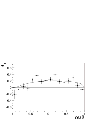
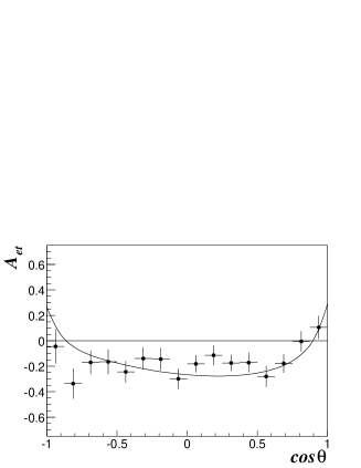
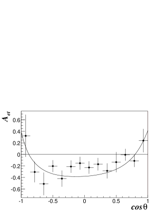
Figure 11: The beam-target asymmetries $A_{t}$(upper half)) and $A_{et}$(lower half) (as defined in Ref.biselli ) of $p(e,e^{\prime}\pi^{0})p$ reaction as a function of $\cos\theta^{*}$ integrated over $\phi^{*}$ at $W=1.22$ GeV and
$0.5$ (GeV/c)² $<$ Q² $<0.9$ (GeV/c)² (left), $0.9$ (GeV/c)² $<$ Q² $<1.5$ (GeV/c)² (right). $(\theta^{*},\phi*$) are the pion angles in the center of mass frame of the final $\pi N$ system. The solid curves are the predictions of the SL model. The data are from Biselli et al. biselli

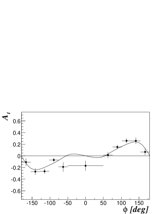
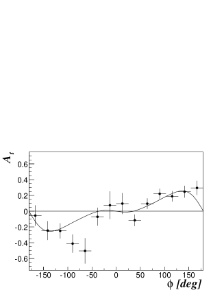
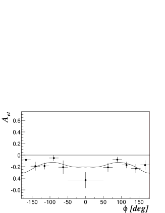
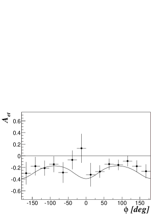
Figure 12: The beam-target asymmetries $A_{t}$(upper half)) and $A_{et}$(lower half) (as defined in Ref.biselli ) of $p(e,e^{\prime}\pi^{0})p$ reaction as a function of $\phi^{*}$ integrated over $\cos\theta^{*}$ at $W=1.22$ GeV and
$0.5$ (GeV/c)² $<$ Q² $<0.9$ (GeV/c)² (left), $0.9$ (GeV/c)² $<$ Q² $<1.5$ (GeV/c)² (right). $(\theta^{*},\phi*$) are the pion angles in the center of mass frame of the final $\pi N$ system. The solid curves are the predictions of the SL model. The data are from Biselli et al. biselli .

Figure 13: Spin dependent structure functions $g_{1}$ (left) and $g_{2}$ (right) for the proton target. The dashed curves are from the fits to the deeply inelastic scattering data as explained in the text. The solid curves are the results at $Q^{2}=0.21,0.35,0.62,0.92,1.37$ (GeV/c)² (from left to right) calculated from the SL model. The data for $g_{1}$ are from Fatemi et al. fatemi .

Figure 14: The parity violating aymmetry terms $\Delta_{A}$(solid curve) and $-\Delta_{V}$(dotted curve) (defined in Eqs.(53)-(54)) of $p(\vec{e},e^{\prime})$ as a function of invariant mass $W$ calculated from the extended SL model described in this work. The results are for incident electron energy $E=1$ GeV and scattering angle $\theta=110^{o}$.

Figure 15: The parity violating asymmetry terms $\Delta_{A}$(solid curves) and $\Delta_{V}$(dotted curves) (defined in Eqs.(53)-(54)) of $p(\vec{e},e^{\prime})$ as a function of the incident electron energy $E_{e}$ calculated from the extended SL model described in this work. The results are for invariant mass $W=1.232$ GeV and electron scattering angles $\theta=60^{o}$(left) and $\theta=110^{o}$(right).

Figure 16: The parity violating asymmetry term $\Delta_{A}$ (defined in Eq. (54)) of $p(\vec{e},e^{\prime})$ as a function of $Q^{2}$ evaluated with an invariant mass $W=1.232GeV$ and electron scattering angle $\theta=110^{o}$. The solid curve is from the extended SL model described in this work. The dashed curve is from turning off the pion cloud effect on the axial $N$-$\Delta$ transition. The dotted curve near the bottom is from keeping only the non-resonant amplitude in the calculation.

Figure 17: The $Q^{2}$-dependence of the scaled parity violating asymmetry $A/Q^{2}$ of $p(\vec{e},e^{\prime})$ calculated from the extended SL model described in this work. The results are for $W=1.232$ GeV and incident electron energy E= 0.8 (solid curve), 1.5 (dotted), 2.0 (dashed), 4.0 (dash-dotted)

Figure 18: The scaled parity violating asymmetry $A/Q^{2}$ of $p(\vec{e},e^{\prime})$ calculated from the extended SL model described in this work. The solid (dashed) curve is from using the axial $N$-$\Delta$ form factor $G^{A}_{N,\Delta}$ of Ref.sl3 ( Refs.kitagaki ). The results are for invariant $W$=1.232 GeV and electron angle $\theta=110^{o}$.

Figure 19: The scaled parity violating asymmetry $A/Q^{2}$ of $p(\vec{e},e^{\prime})$ as a function of the scaling variable $\xi$ predicted by the extended SL model described in this work (solid curves) is compared with that calculated from Eqs.(55)-(59) using the CTEQ6 parton distribution functions (dashed curves). The results are for $E=4$ GeV ,$Q^{2}=0.5$ (GeV/c)² (top left), $E=6$ GeV ,$Q^{2}=1$ (GeV/c)² (top right), $E=8$ GeV, $Q^{2}=5$ (GeV/c)² (bottom left), and $E=12$ GeV, $Q^{2}=10$ (GeV/c)² (bottom right).

References

• (1) T. Sato and T.-S. H. Lee, Phys. Rev. C 54, 2660 (1996).
• (2) T. Sato and T.-S. H. Lee, Phys. Rev. C 63, 055201 (2001).
• (3) T. Sato, D. Uno and T.-S. H. Lee, Phys. Rev. C67, 065201 (2003).
• (4) E. D. Bloom and F. J. Gilman, Phys. Rev. Lett. 25, 1140 (1970).
• (5) J.G. Morfin, Nucl. Phys. B112, 251 (2002).
• (6) S.P. Well, N. Simicevic, K. Johnson and The G0 Collaboration, proposal PR-04-101, Jefferson Laboratory (2004).
• (7) P. Bosted et al, proposal PR-05-005, Jefferson Laboratory (2005).
• (8) W. Melnitchouk, R. Ent, and C. E. Keppel, Phys. Rep. 406, 127 (2005).
• (9) I. Niculescu et al., Phys. Rev. Lett. 85, 1186 (2000).
• (10) Y. Liang et al. , arXiv:nucl-ex/0410027 v1 (2004).
• (11) O. Nachtmann, Nucl. Phys. B63, 237 (1973).
• (12) H. Georgi and H. D. Politzer, Phys. Rev. D 14, 1829 (1976).
• (13) A. De Rujula, H. Georgi, and H. D. Politzer, Phys. Lett. B 64, 428 (1976); Annuals Phys. 103, 315 (1977).
• (14) X. Ji and P. Unrau, Phys. Rev. D 52, 72 (1995).
• (15) X. Ji and W. Melnitchouk, Phys. Rev. D 56, R1 (1997).
• (16) A. Mueller, Phys. Lett. B 308, 355 (1993).
• (17) C.E. Carlson and N.C. Mukhopadhyay, Phys. Rev. Lett. 74, 1288 (1995); Phys. Rev. D 58, 094029 (1998).
• (18) J. Edelmann, G. Piller, N. Kaiser, and W. Weise, Nucl. Phys. A665, 125 (2000).
• (19) W. Melnitchouk, K. Tsushima, A.W. Thomas, Eur. Phys. J. A14, 105 (2002).
• (20) For Standard model, see, for example, Dynamics of the Standard Model, by J. F. Donoghue, E. Golowich, and B. R. Holstein, 1992 (Cambridge University Press)
• (21) A. Biselli et al., Phys. Rev. C 68, 035202 (2003).
• (22) K. Joo et al., Phys. Rev. C 70, 042201 (2004).
• (23) R. Fatemi et al., Phys. Rev. Lett. 91, 222002 (2003).
• (24) K. Abe et al., Phys. Rev. D 58, 112003 (1998).
• (25) S. Wandzura and F. Wilczek, Phys. Lett. B 72, 195 (1977).
• (26) V. Burkert and T.-S. H. Lee, Int.J.Mod.Phys E13, 1035-1112 (2004).
• (27) T. Kitagaki et al., Phys. Rev. D 42, 1331 (1990); an other references there in.
• (28) T.R. Hemmert, B.R. Holstein, and N.C. Mukhopadhyay, Phys. Rev. D 51, 158 (1995).
• (29) J. Liu, N.C. Mukhopadhyay, and L. Zhang, Phys. Rev. C 52 1630 (1995).
• (30) B. Golli, S. Sirca, L. Amoreira and M. Fiolhais, Phys. Lett. B553, 51 (2003).
• (31) B. Julia-Diaz, D.O. Riska, and F. Coester, Phys. Rev. C70, 045204 (2004).
• (32) R.N. Cahn and F.J. Gilman, Phys. Rev. D17, 1313 (1978).
• (33) D.R.T. Jones and S.T. Petcov, Phys. Lett B91, 137 (1980).
• (34) D. Ishankuliev and M. Ya. Safin, Sov. J. Nucl. Phys. 31, 512 (1980).
• (35) S.P. Li, E.M. Henley, and W.-Y. P. Hwang, Ann. Phys. (NY) 143, 371 (1982).
• (36) L.M. Nath, K. Schilcher, M. Kretzschmar, Phys. Rev. D25, 2300 (1982).
• (37) M.J. Musolf et al., Phys. Rep. 239, 1 (1994).
• (38) H-W. Hammer and D. Drechsel, Z. Phys. A353, 321 (1995).
• (39) N.C.Mukhopadhyay, M.J. Ramsey-Musolf, S.J. Pollock, J. Liu, and H.-W. Hammer, Nucl. Phys. A633, 481 (1998).
• (40) M.P. Rekalo, J. Arvieux, and E.Tomasi-Gustafsson, Phys. Rev. C65, 035501 (2002).
• (41) A.W. Thomas and W. Weise, The Structure of the Nucleon, 2001 (Wiley-VCH)
• (42) J. Gasser and H. Leutwyler, Ann. Phys. 158, 142 (1984).
• (43) T.-S. Park et al., Phys. Rep. 233, 341 (1993).
• (44) V. Bernard et al., J. Phys. G 28, R1 (2002).
• (45) J. Pumplin, D.R. Stump, J. Huston, H.L. Lai, P. Nadolsky, and W.K. Tung, Journal of High Energy Physics, 0207, 012 (2002) (hep-ph/0201195 ).
• (46) X. Ji, Phys. Lett. B309, 187 (1993).
• (47) R. Barbiberi, J. R. Ellis, M. K. Gaillard, and G.G. Ross, Nucl. Phys. B 117, 50 (1976); S. Dasu et al., Phys. Rev. D 49, 5641 (1994).
• (48) J. Arrington et al., Phys. Rev. C64, 014602 (2001).
• (49) F. W. Brase et al. Nucl. Phys. B110, 410 (1976).
• (50) P. Stoler, Phys. Rev. D 44, 73 (1991).
• (51) S. Nozawa and T.-S. H. Lee, Nucl. Phys. A 513, 543 (1990).
• (52) R. Fatemi, priviate communications.
• (53) Y. Goto et al, Phys. Rev. D62, 034017 (2000); M. Hirai, S. Kumano and N. Saito, Phys. Rev. D69, 054021 (2004).
• (54) M. Anselmino, B.L. Ioffe, and E. Leader, Yad. Fiz. 49, 214 (1989)[Sov. J. Nucl. Phys. 49, 136 (1989)]; F. Close, in Excited Baryons 1988, Proceedings of the Topical Workshop on Excited Baryons, edited by G. Adams, N.C. Mukhopadhyay, and P. Stoler (World Scientific, Singapore, 1989); V. D. Burkert and B. L. Ioffe, J. Exp. Theore. Phys. 78, 619 (1994).
• (55) J. Ellis and R. Jaffe, Phys. Rev. D 9, 1444 (1974).
• (56) S. D. Drell and A.C. Hearn, Phys. Rev. Lett. 16, 908 (1966); S. B. Gerasimov, Sov. J. Nucl. Phys. 2, 598 (1966).
• (57) P.L. Anthony et al. , Phys. Lett. B553, 18 (2003).
• (58) J. Erler and P. Langacker, Particle Data Group, Phys. Rev. D 66, 010001 (2002).
Refer to caption