Strange form factors and Chiral Perturbation Theory

Abstract

We review the contributions of Chiral Perturbation Theory to the theoretical understanding or not-quite-yet-understanding of the nucleon matrix elements of the strange vector current.

1 Introduction

Chiral Perturbation Theory (ChPT), as the low-energy effective field theory of the Standard Model, ought to be predestined to describe the response of the nucleon to the strange vector current: it incorporates all symmetry constraints of the fundamental theory and contains the degrees of freedom relevant at low energies, Goldstone bosons (pions and kaons) as well as matter fields (nucleons). In Sect. 2, we shall point out some specific aspects of ChPT that are essential for the following discussion. We shall reiterate in Sect. 3 why symmetry considerations alone are not sufficient for ChPT to be predictive for the leading moments of the strange form factors, the strange magnetic moment $\mu_{s}$ and the strange electric radius $\langle r_{E,s}^{2}\rangle$. A low-energy theorem for the strange magnetic radius $\langle r_{M,s}^{2}\rangle$ is presented in Sect. 4, its usefulness and limitations are discussed. Some alternative regularization schemes for loop diagrams have been suggested in order to achieve improved convergence behavior of the chiral series, we shall say a few words on these in Sect. 5. Finally, a conclusion is given in Sect. 6.

2 Some aspects of Chiral Perturbation Theory

2.1 Goldstone bosons and counterterms

ChPT gl systematically exploits the far-reaching consequences of chiral symmetry: it dictates the appearance of (pseudo) Goldstone bosons ($\pi$, $K$, $\eta$) and tightly constrains their interaction with each other as well as with external currents and matter fields. As a consequence, the Goldstone boson dynamics is completely calculable, while the influence of heavier states can be parameterized, at low energies, by polynomials. The polynomial coefficients (called low-energy constants) are not numerically known a priori, but are still far from arbitrary, as they potentially interrelate many different observables. A particularly famous example is the quark mass expansion of the pion mass:

$$M_{\pi}^{2}=2B\hat{m}-\frac{\bar{\ell}_{3}}{32\pi^{2}F_{\pi}^{2}}\bigl{[}2B\hat{m}\bigr{]}^{2}+\mathcal{O}\left(\hat{m}^{3}\right)~{}~{},$$ (1)

where $\hat{m}=(m_{u}+m_{d})/2$. The first term on the right constitutes the well-known Gell-Mann–Oakes–Renner relation. The correction of order $\hat{m}^{2}$ is proportional to the low-energy constant $\bar{\ell}_{3}$ that can be determined from $\pi\pi$ scattering. Given such independent experimental information, the relative size of the contributions to $M_{\pi}^{2}$ linear and quadratic in the quark masses is known condensate .

2.2 Power counting

In the Goldstone boson sector of ChPT, Lorentz invariance dictates that only even powers of momenta appear in the effective Lagrangian. The typical low-energy expansion parameters therefore are $M_{\pi}^{2}/\Lambda_{\chi}^{2}\approx 0.02$ (for chiral SU(2)) or $M_{K}^{2}/\Lambda_{\chi}^{2}\approx 0.2$ (for chiral SU(3)), where the chiral symmetry breaking scale is $\Lambda_{\chi}=4\pi F_{\pi}\approx 1160$ MeV. In contrast, due to the appearance of spin, there are also odd powers of momenta in the effective pion-nucleon Lagrangian, such that the convergence order-by-order is markedly slower, typical expansion parameters are $M_{\pi}/m_{N}\approx 0.15$ in SU(2) or $M_{K}/m_{N}\approx 0.5$ for SU(3). Obviously, there is no way we can expect ChPT to work as well for the baryon sector with strangeness as it does for, say, $\pi\pi$ scattering.

It is important to understand the “generic” chiral orders of the lowest moments in the nucleon vector form factors, i.e. the orders at which polynomial contributions occur. The low-energy expansion of the strange Sachs form factors is given by

$$G_{E,s}\left(Q^{2}\right) = \underbrace{\phantom{\frac{1}{6}}\hskip-8.5359ptQ_{s}}_{\mathcal{O}(p)}-\;\underbrace{\frac{1}{6}\langle r_{E,s}^{2}\rangle\,Q^{2}}_{\mathcal{O}(p^{3})}\,\,+\,\ldots~{}~{},$$

$$G_{M,s}\left(Q^{2}\right) = \underbrace{\phantom{\frac{1}{6}}\hskip-8.5359pt\mu_{s}}_{\mathcal{O}(p^{2})}\!-\;\underbrace{\frac{1}{6}\langle r_{M,s}^{2}\rangle\,Q^{2}}_{\mathcal{O}(p^{4})}\,+\,\ldots~{}~{},$$

where one has $Q_{s}=0$ due to gauge invariance for the strange charge. We note in particular that polynomial contributions to the radius terms $\langle r_{E,s}^{2}\rangle$, $\langle r_{M,s}^{2}\rangle$ appear at leading and subleading one-loop order, respectively.

3 Why ChPT cannot predict $\mu_{s}$ and $\langle r_{E,s}^{2}\rangle$

The reason why it is impossible to predict $\mu_{s}$ and $\langle r_{E,s}^{2}\rangle$ from first principles in ChPT was identified several years ago ito . There are three independent diagonal vector currents in SU(3),

$$J_{\mu}^{(i)}=\bar{q}\frac{\lambda^{i}}{2}\gamma_{\mu}q~{}~{},\qquad i=3,\,8,\,0,$$ (2)

where $\lambda^{3/8}$ are the usual Gell-Mann matrices and $\lambda^{0}=\sqrt{2/3}\;{\rm diag}(1,1,1)$. The three are proportional to the isovector and isoscalar electromagnetic currents and the baryon number current, respectively. The electromagnetic and the strangeness currents are linear combinations of these,

$$J_{\mu}^{\rm EM}=J_{\mu}^{(3)}+\frac{1}{\sqrt{3}}J_{\mu}^{(8)}~{}~{},\quad J_{\mu}^{s}=\sqrt{\frac{2}{3}}J_{\mu}^{(0)}-\frac{2}{\sqrt{3}}J_{\mu}^{(8)}~{}~{},$$ (3)

i.e. the response to one component of the strangeness current, the baryon number, is going to be completely independent of what we know from electromagnetic probes. In the effective Lagrangian language, this means that wherever matrix elements of the electromagnetic current depend on low-energy constants, there will be a new, independent constant for the strangeness current. As an example, consider the leading terms contributing to the magnetic moments,

$$\mathcal{L}^{(2)}=\frac{b_{6}^{D/F}}{8m_{N}}\langle\bar{B}\sigma^{\mu\nu}\left[F_{\mu\nu}^{+},B\right]_{\pm}\rangle+\frac{b_{6}^{0}}{8m_{N}}\langle\bar{B}\sigma^{\mu\nu}B\rangle\langle F_{\mu\nu}^{+}\rangle~{}.$$ (4)

The constants $b_{6}^{D/F}$ can be fitted alternatively to the magnetic moments of proton and neutron or to all octet moments, but $b_{6}^{0}$ only appears in the strange magnetic moment. The same pattern emerges for all low-energy constants, therefore instead of predicting the strange vector form factors, ChPT can only adjust its constants in order to reproduce experimental findings.

4 The strange magnetic radius

Besides being a quantity of interest in its own right, the strange magnetic radius $\langle r_{M,s}^{2}\rangle$ is also of high importance for the experimental determination of the strange magnetic moment $\mu_{s}$ for the following reason: Experimental measurements of $G_{M,s}(Q^{2})$ always have to be performed at finite, non-vanishing $Q^{2}$, therefore one needs to extrapolate to $G_{M,s}(0)=\mu_{s}$ HMS .

4.1 A low-energy theorem for $\langle r_{M,s}^{2}\rangle$

Figure 1: Diagram generating the leading contribution to $\langle r_{M,s}^{2}\rangle$

After the pessimistic finding of the last section, how can there possibly be any low-energy theorem for any strange vector form factor? The answer is, through leading non-analytic loop effects. The diagram of order $\mathcal{O}(p^{3})$ displayed in Fig. 1 generates a contribution to the strange magnetic radius according to HMS

$$\langle r_{M,s}^{2}\rangle^{(3)}=-\frac{5D^{2}-6DF+9F^{2}}{48\pi F_{K}^{2}}\frac{m_{N}}{M_{K}}+\mathcal{O}(M_{K}^{0})~{}~{}.$$ (5)

As a low-energy constant can only contribute to $\langle r_{M,s}^{2}\rangle$ at the next order, generating a term of $\mathcal{O}(M_{K}^{0})$, the term in (5) is (at least formally) dominant. All the masses and coupling constants in (5) are known, hence we have a parameter-free prediction for $\langle r_{M,s}^{2}\rangle$,

$$\langle r_{M,s}^{2}\rangle=-0.115~{}{\rm fm}^{2}~{}~{}.$$ (6)

We can use the leading chiral prediction for $\langle r_{M,s}^{2}\rangle$ to extrapolate from the SAMPLE result sample $G_{M,s}(0.1\,{\rm GeV}^{2})=0.37\pm 0.20\pm 0.26\pm 0.07$ to the strange magnetic moment,

$$\mu_{s}=0.32\pm 0.20\pm 0.26\pm 0.07~{}~{}.$$ (7)

This extrapolation is visualized in Fig. 2.

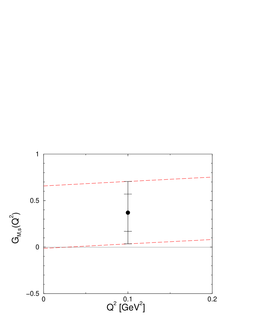
Figure 2: Extrapolation of the SAMPLE value $G_{M,s}(Q^{2})$ to $\mu_{s}$

Figure 3: $Q^{2}$–dependence of $G_{E,s}$ at $\mathcal{O}(p^{3})$. The figure is taken from HKM

Furthermore, in HKM this was combined with a second experimental result, the HAPPEX measurement happex for $G_{E,s}+0.39G_{M,s}$, in order to fix both unknowns in the $\mathcal{O}(p^{3})$ representation of the strange form factors (for $\mu_{s}$ and $\langle r_{E,s}^{2}\rangle$) and predict also the $Q^{2}$–dependence of the strange electric form factor, see Fig. 3. We note from that figure that even over a large $Q^{2}$ range, the form factor looks essentially linear and displays only very little curvature. The reason for this is that the closest infrared singularity in this representation is the $K\bar{K}$ cut, which has a threshold far away from the physical region, and that counterterms providing curvature in the polynomial part are suppressed to two-loop order.

4.2 Stability of the low-energy theorem

Even though the low-energy theorem (5) is strictly a theorem, it is an important problem to study its stability when subject to higher-order corrections. A calculation to $\mathcal{O}(p^{4})$ has been performed hammer (see also diss ), from which we only quote the numerical result,

$$\langle r_{M,s}^{2}\rangle^{(4)}=-\bigl{(}0.04+0.3\,b_{s}^{r}\bigr{)}~{}{\rm fm}^{2}~{}~{},$$ (8)

where the low-energy constant $b_{s}^{r}$ is expected to be of order 1. We note that the corrections to the central value as compared to (6) are sizeable, and that the unknown constant induces a theoretical uncertainty in the extraction of $\mu_{s}$ from experiment. The corresponding plot is shown in Fig. 4 (taken from hammer ).

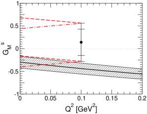
Figure 4: Extrapolation of the SAMPLE value $G_{M,s}(Q^{2})$ to $\mu_{s}$, using the $\mathcal{O}(p^{4})$ value for $\langle r_{M,s}^{2}\rangle$. The grey band indicates a dispersion-theoretical prediction. The figure is taken from hammer

5 Variants of loop regularization

We have seen that the low-energy theorem for $\langle r_{M,s}^{2}\rangle$ is given by a leading-order kaon-loop effect, but that the next-to-leading order corrections are sizeable. We therefore want to discuss here two alternative schemes to evaluate loops that may resum these corrections more efficiently, or may give a fairer estimate of these contributions altogether.

5.1 Infrared regularization

All loop results discussed so far have been calculated in what is called Heavy Baryon Chiral Perturbation Theory. In this formalism, the nucleons are treated as heavy, non-relativistic fields, for which the relativistic corrections suppressed by powers of $1/m_{N}$ can be calculated systematically. This method has the advantage that loop diagrams always follow naive power counting rules and that leading loop calculations are technically simple, but the downside that the analytic structure is sometimes distorted even in the low-energy region, and that in practice $1/m_{N}$ corrections are awkward to calculate.

One alternative scheme that has been suggested to overcome these shortcomings is “infrared regularization” becher , which is a variant of dimensional regularization that preserves power counting also in relativistic baryon ChPT. In this scheme, all the $1/m_{N}$ corrections are automatically resummed as depicted schematically in Fig. 5.

Figure 5: Resummation of relativistic corrections in the infrared regularization scheme. The crosses denote $1/m_{N}$ insertions in the nucleon propagator

It has been shown in irff that in some cases particularly sensitive to relativistic “recoil effects” (in irff : the neutron electric form factor), this relativistic resummation leads to a much improved convergence behavior. It is therefore interesting to see what happens to the strange magnetic radius in this scheme, even beyond $\mathcal{O}(p^{4})$. We find the following partial corrections of $\mathcal{O}(p^{5})$ diss :

$$\Delta\langle r_{M,s}^{2}\rangle^{(5)} = -\frac{35(5D^{2}\!-\!6DF\!+\!9F^{2})}{384\pi F_{K}^{2}}\frac{M_{K}}{m_{N}}+\mathcal{O}\biggl{(}\!\frac{\Delta m_{\Lambda/\Sigma}}{M_{K}}\!\biggr{)}$$ (9)

$$= +0.053~{}{\rm fm}^{2}~{}~{},$$

where the additional terms proportional to $\Delta m_{\Lambda/\Sigma}=m_{\Lambda/\Sigma}-m_{N}$ have been included in the numerical value. Although these expressions are not complete (there will also be two-loop contributions), they are non-analytic in the quark masses and therefore not modified by counterterms. Numerically, they turn out to be large, about half the size of the leading $\mathcal{O}(p^{3})$ value. This supports once more the conclusion that, unfortunately, the low-energy theorem for $\langle r_{M,s}^{2}\rangle$ at $\mathcal{O}(p^{3})$ is numerically not very reliable.

5.2 Cutoff regularization

Various attempts at cutoff regularization have been undertaken in the context of ChPT. We do not try to give an overview of these, but instead concentrate on one specific approach cutoff in which $\langle r_{M,s}^{2}\rangle$ has explicitly been considered umass . The idea is that the nucleon has an intrinsic size, and that ChPT can only reliably predict the $\pi$ or $K$ fluctuations that are long-ranged on this scale. Dimensional regularization does not separate these different ranges of momenta in the loop integration, such that it might be more efficient to employ a cutoff in order to reduce unrealistically strong short-distance effects.

The method in cutoff amounts to the use of a $KNN$ form factor instead of a constant vertex. In umass , a dipole form has been chosen, which leads to the analytic result

$$\langle r_{M,s}^{2}\rangle_{\rm cutoff} = \langle r_{M,s}^{2}\rangle_{\rm dim.reg.}\times X\bigl{(}{\textstyle\frac{\Lambda}{M_{K}}}\bigr{)}~{}~{},$$ (10)

$$X(x) = \frac{x^{3}(x^{2}+\frac{14}{5}x+1)}{(x+1)^{5}}~{}~{}.$$

This cutoff dependence is displayed in Fig. 6. It is obvious that for cutoffs of the order of $\Lambda=400\ldots 600$ MeV, $\langle r_{M,s}^{2}\rangle_{\rm cutoff}$ is sizeably reduced compared to the dimensional regularization result.

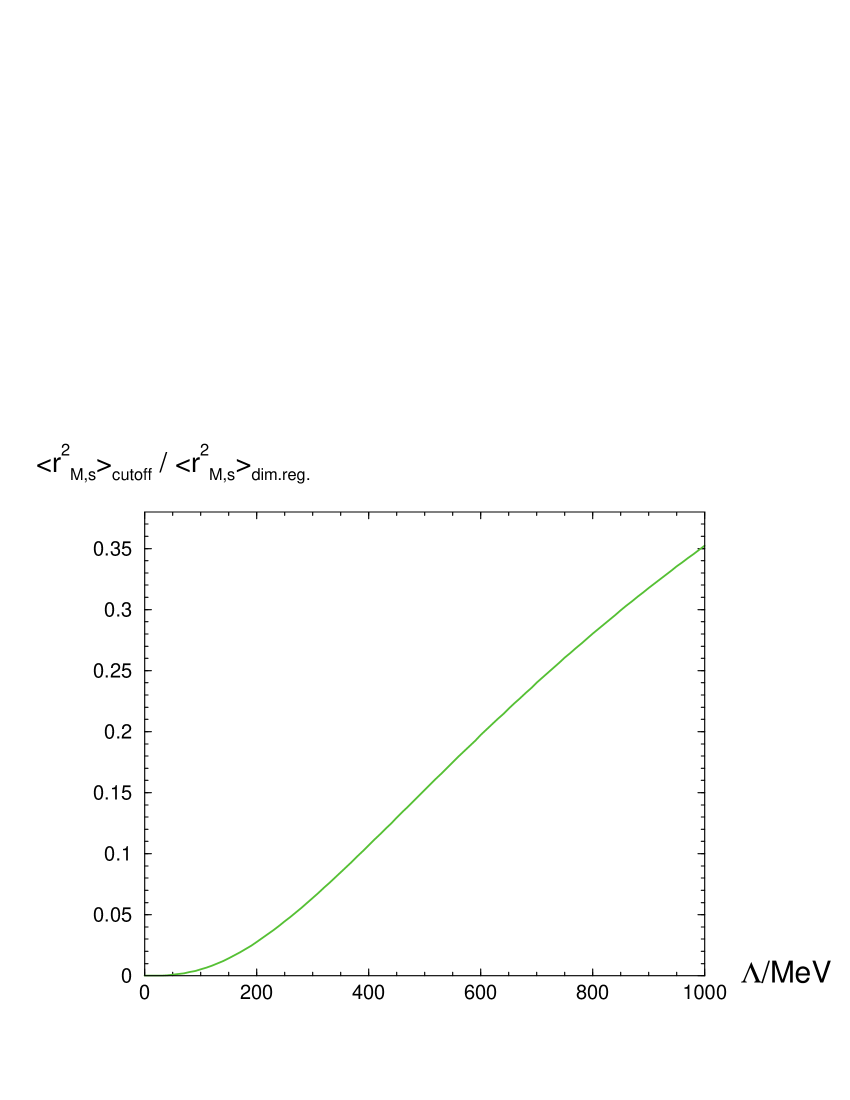
Figure 6: Cutoff dependence of $\langle r_{M,s}^{2}\rangle$

Despite the host of plausible arguments in favor of cutoff schemes, there are also some drawbacks:

1. The cutoff is an additional parameter that can only, at best, be estimated.

2. It presents a deviation from the strict effective Lagrangian approach in ChPT, as a consequence of which gauge invariance usually has to be cured “by hand”, and chiral symmetry is by no means guaranteed.

3. The cutoff upsets the analytic structure of the form factors: it produces additional unphysical poles and/or cuts. This means in particular that is is unclear how a marriage with dispersion relations (see e.g. hammer and references therein) might be achieved.

4. Finally, the reduction of the numerical value of $\langle r_{M,s}^{2}\rangle$ must not be confused with the inclusion of higher order corrections as done in the infrared regularization scheme. The problem of large $1/m_{N}$ corrections in chiral SU(3) is by no means solved here.

6 Summary and conclusions

The matrix elements of the strange vector current seem to remain elusive quantities for a description in Chiral Perturbation Theory. They are problematic as Goldstone boson dynamics is not overly dominant here, and in most cases, unknown low-energy constants appear at leading order. We have pointed out that there is an exception, the strange magnetic moment for which a parameter-free low-energy theorem exists. However, higher order corrections are found to be sizeable, such that the low-energy theorem is very unstable once these are taken into account. Also cutoff calculations indicate a smaller absolute size of $\langle r_{M,s}^{2}\rangle$. The role of ChPT remains however to aid to interrelate more data, as they become available a4 .

Acknowledgements. I would like to thank the organizers of PAVI 04 for the great opportunity to participate in this workshop, and for the wonderful organization of the whole event. I am grateful to T.R. Hemmert and U.-G. Meißner for the fruitful collaboration that originally introduced me to this subject, and to various colleagues for interesting discussions that deepened my understanding of the field, in particular H.-W. Hammer, M.J. Ramsey-Musolf, J.F. Donoghue, B.R. Holstein, T. Huber, and A. Roß. This work was supported in part by RTN, BBW-Contract No. 01.0357, and EC-Contract HPRN–CT2002–00311 (EURIDICE).

References

- (1) J. Gasser, H. Leutwyler: Annals Phys. 158 (1984) 142; J. Gasser, H. Leutwyler: Nucl. Phys. B 250 (1985) 465
- (2) G. Colangelo, J. Gasser, H. Leutwyler: Phys. Rev. Lett. 86 (2001) 5008
- (3) M.J. Musolf, H. Ito: Phys. Rev. C 55 (1997) 3066
- (4) T.R. Hemmert, U.-G. Meißner, S. Steininger: Phys. Lett. B 437 (1998) 184
- (5) D.T. Spayde et al. [SAMPLE Collaboration]: Phys. Lett. B 583 (2004) 79
- (6) K. A. Aniol et al. [HAPPEX Collaboration]: Phys. Rev. Lett. 82 (1999) 1096; Phys. Lett. B 509 (2001) 211
- (7) T.R. Hemmert, B. Kubis, U.-G. Meißner: Phys. Rev. C 60 (1999) 045501
- (8) H. W. Hammer, S. J. Puglia, M. J. Ramsey-Musolf, S. L. Zhu: Phys. Lett. B 562 (2003) 208
- (9) B. Kubis: Thesis, Berichte des FZ Jülich, Jül-4007 (2002)
- (10) T. Becher, H. Leutwyler: Eur. Phys. J. C 9 (1999) 643
- (11) B. Kubis, U.-G. Meißner: Nucl. Phys. A 679 (2001) 698
- (12) J.F. Donoghue, B.R. Holstein, B. Borasoy: Phys. Rev. D 59 (1999) 036002
- (13) T. Huber: Master thesis (Univ. of Massachusetts, 2002); A. Roß: Master thesis (Univ. of Massachusetts, 2003)
- (14) D. Djukanovic, M. R. Schindler, J. Gegelia, S. Scherer: (2004), arXiv:hep-ph/0407170
- (15) F. E. Maas et al. [A4 Collaboration]: Phys. Rev. Lett. 93 (2004) 022002