Density inhomogeneities in heavy ion collisions around the critical point

Abstract

We study the hydrodynamical expansion of a hot and baryon-dense quark fluid coupled to classical real-time evolution of the long wavelength modes of the chiral field. Significant density inhomogeneities develop dynamically when the transition to the symmetry-broken state occurs. We find that the amplitude of the density inhomogeneities is larger for expansion trajectories crossing the line of first-order transitions than for crossovers, which could provide some information on the location of a critical point. A few possible experimental signatures for inhomogeneous decoupling surfaces are mentioned briefly.

I Introduction

Heavy ion collisions at high energies produce hot and baryon-dense strongly interacting matter and so provide the opportunity to explore the phase diagram of QCD HIPhaseTrans . Recent lattice QCD calculations at finite baryon-chemical potential Fodor:2004nz indicate that at sufficiently large baryon density a line of first order transitions exists in the plane of temperature $T$ versus baryon-chemical potential $\mu_{B}$. This line separates the region where chiral symmetry is broken (as in vacuum) from that where it is approximately restored. Moving counter-clockwise along this phase boundary, i.e. towards higher $T$ and lower $\mu_{B}$, results in weaker first-order transitions and finally the line of first order transition ends at a second-order critical point SRS . Simulations with semi-realistic quark masses locate the endpoint at $T_{E}\simeq 160$ MeV, $\mu_{B,E}\simeq 360$ MeV. For $\mu_{B}<\mu_{B,E}$ no phase transition in the strict sense occurs. Rather, the low- and high-temperature phases are continuously connected by a rapid crossover.

Our goal here is to analyze the homogeneity of the “fluid” of QCD matter as it expands and cools. In particular, we shall study expansion trajectories passing on either side of the critical point (i.e. either crossover or first order phase transition). As we will show, in the vicinity of the critical point the expanding fluid develops significant inhomogeneities. Such density perturbations should also be present on the decoupling surface of hadrons. This is normally neglected in hydrodynamical simulations of heavy-ion collisions, which commonly assume that the hadrons freeze out at a fixed temperature or density.

The fact that decoupling surfaces are typically not homogeneous is well known. Take, for example, the WMAP data on the temperature fluctuations of the cosmic microwave background (CMB) wmap . The background photons exhibit temperature fluctuations on the order of $\Delta T/T\simeq 10^{-5}$. From the CMB multipoles one hopes to gather information on their primordial origin. In heavy-ion collisions, on the other hand, we might get hints about the QCD phase transition, if it occurs shortly before decoupling. The basic idea is that if a phase transition occurs then it might leave imprints on the (energy-) density distribution on the freeze-out hypersurface. In particular, we expect the inhomogeneities to be smaller for crossovers and stronger for first order transitions.

The first source of spatial density inhomogeneities in heavy-ion collisions is due to fluctuations in the number of participants and the number of collisions among the beam nucleons. Those fluctuations lead to an inhomogeneous deposition of energy and of baryon number at central rapidity. From the event generator UrQMD, energy density inhomogeneities on the order of $\Delta e\sim 1$ GeV/fm³ have been predicted for central Pb+Pb collisions at top SPS energy ($\surd s\simeq 17A$ GeV) which originate from fluctuations in “soft” (low momentum transfer) interactions; see fig. 4 in Bleicher:wd . At RHIC energies ($\surd s\simeq 100-200A$ GeV) $\Delta e$ could increase by up to an order of magnitude due to the additional semi-hard (“minijet”) component, as discussed in ref. GyRiZ . These authors also discussed the evolution of such initial-state inhomogeneities using equilibrium hydrodynamics in the ideal fluid approximation. They find that even the huge initial perturbations predicted by the minijet model are strongly washed out until freeze out by the hydrodynamic expansion of the hot matter. Qualitatively, this can be understood from the following simple argument. The radius $L\simeq 1$ fm of a hotspot grows linearly in time while its density drops inversely proportional to its volume so that $\Delta\rho\sim 1/t^{3}$ for expansion in three dimensions. The overall duration of the hydrodynamic expansion is expected to be (at least) on the order of the radius of the colliding nuclei HIPhaseTrans ; HK , roughly $\sim 5L$. Therefore, any initial density concentration should be diluted by about a factor of $100$. Hence, initial perturbations of order one would leave traces on the percent level only, at the time of decoupling. For other studies of early-stage density inhomogeneities and their hydrodynamic evolution see refs. Drescher:2000ec and Socolowski:2004hw , respectively comment .

Here, we discuss a different source of density inhomogeneities, namely those possibly generated in the course of a non-equilibrium transition from a (nearly) chirally symmetric state at high temperature and density to the state of broken symmetry at decoupling. The rather rapid transition expected to occur in high-energy heavy-ion collisions very likely forces the long wavelength modes of the chiral condensate out of equilibrium. This should then reflect in a rather non-uniform distribution of energy and baryon density in space (or, more precisely, on the decoupling hypersurface). Most notably, since “freeze out” (decoupling of all particles) in heavy-ion collisions occurs shortly after the transition to the broken phase, such perturbations generated in the late stages of the evolution could largely survive and leave detectable traces in the final state. In this regard, we also recall the results of ref. Bot Aichelin who employed the collisionless Vlasov equation to study the real-time evolution of small initial density fluctuations within the NJL model. They observed an increase of the fluctuations already for the case where the expectation value of the chiral condensate was fixed to its equilibrium value, cf. their eq. (2). Here, we also treat the non-equilibrium dynamics of the chiral condensate, cf. our eq. (4) below, which probes the structure of the effective potential in the vicinity of the critical point.

II The Model

For the current studies we extend the model from ref. Paech:2003fe to allow for nonvanishing baryon density $\rho$. The Gell-Mann-Levy Lagrangian GML

$${\cal L} = \overline{q}\,\left[i\gamma^{\mu}\partial_{\mu}-g(\sigma+\gamma_{5}\vec{\tau}\cdot\vec{\pi})\right]\,q$$ (1)

$$+ \frac{1}{2}\left(\partial_{\mu}\sigma\right)^{2}+\frac{1}{2}\left(\partial_{\mu}\vec{\pi}\right)^{2}-U(\sigma,\vec{\pi})\quad.$$

provides an effective theory for chiral symmetry breaking in QCD. It describes the interaction of two flavors of constituent quarks $q=(u,d)$ with the chiral field $\phi_{a}=(\sigma,\vec{\pi})$. The potential, which exhibits both spontaneously and explicitly broken chiral symmetry, is

$$U(\sigma,\vec{\pi})=\frac{\lambda^{2}}{4}(\sigma^{2}+\vec{\pi}^{2}-{\it v}^{2})^{2}-h_{q}\sigma-U_{0}\quad.$$ (2)

The vacuum expectation values of the condensates are $\langle\sigma\rangle={\it f}_{\pi}$ and $\langle\vec{\pi}\rangle=0$, where ${\it f}_{\pi}=93$ MeV is the pion decay constant. The explicit symmetry breaking term is due to the non-zero pion mass, $h_{q}=f_{\pi}m_{\pi}^{2}$, where $m_{\pi}=138$ MeV. This leads to $v^{2}=f^{2}_{\pi}-{m^{2}_{\pi}}/{\lambda^{2}}$. The value of $\lambda^{2}=20$ leads to a $\sigma$-mass, $m^{2}_{\sigma}=2\lambda^{2}f^{2}_{\pi}+m^{2}_{\pi}$, approximately equal to 600 MeV.

We assume that the quarks constitute a thermalized fluid, which provides an expanding background in which the long-wavelength modes of the chiral condensate evolve. Integrating out the quarks generates an effective potential for $\phi_{a}$; computing to one loop and for a homogeneous background (on the scale of a “fluid element”), this contribution is given by

$$V_{\rm eff}(\phi,T,\mu) = U(\phi)-d_{q}\;T\int\!\frac{{\rm d}^{3}p}{(2\pi)^{3}}$$

$$\left\{\log\left(1+e^{{(\mu-E)}/{T}}\right)+\left(\mu\rightarrow-\mu\right)\right\}~{}.$$

Here, $d_{q}=12$ denotes the color-spin-isospin degeneracy of the quarks and $\mu=\mu_{B}/3$ the quark-chemical potential. The two terms inside the integral correspond to the thermal contributions of quarks and anti-quarks, respectively; a (divergent) vacuum contribution has been absorbed into the $T$ and $\mu$ independent potential $U$. $V_{\rm eff}$ depends on the order parameter field through the effective mass of the quarks, $m_{q}^{2}=g^{2}\phi^{2}$, which enters the expression for the single-particle energy $E=\sqrt{{\vec{p}}^{\;2}+m^{2}_{q}}$.

For sufficiently small quark-chemical potential $\mu$ one finds a smooth transition to approximately massless quarks at high $T$. For larger chemical potential, however, the effective potential exhibits a first-order phase transition SMMR . Along the line of first-order transitions the effective potential exhibits two degenerate minima which are seperated by a “nucleation barrier”. This barrier decreases with $\mu$ and the two minima approach each other. At $\mu_{E}$, finally, the barrier vanishes, and so does the latent heat. For $g=3.3$, which leads to a constituent quark mass in vacuum of $\approx 307$ MeV, the second-order critical point is located at $T_{E}\approx 100$ MeV, $\mu_{E}\approx 200$ MeV. Increasing the quark-field coupling $g$ moves the endpoint $E$ towards the temperature axis ove ($\mu_{E}$ becomes =0 at about $g\approx 3.7$ Paech:2003fe ) and to slightly higher temperature. In what follows, we fix $g=3.3$.

The location of the endpoint does not agree quantitatively with that from recent lattice QCD studies with realistic quark masses, which find $T_{E}\approx 160$ MeV and $\mu_{E}\approx 120$ MeV Fodor:2004nz . This failure is common to several models, c.f. fig. 6 in stephanov and could be due to the neglect of heavier resonance states in the above effective Lagrangian, see e.g. the discussion in det . Also, if deconfinement and chiral symmetry restoration occur simultaneously then the energy density contributed by Polyakov loops in the deconfined phase should be included as well Ploops . Finally, note that the model fails to describe the nuclear matter ground state, which has non-zero pressure and is located in the phase coexistence region (Fig. 1 below). Nevertheless, one might hope that, qualitatively, the dynamics of relativistic quark fluids near the endpoint is not affected by the deficiencies of this simple model.

The classical equations of motion for the chiral fields are

$$\partial_{\mu}\partial^{\mu}\phi_{a}+\frac{\delta V_{\rm eff}}{\delta\phi_{a}}=0~{}.$$ (4)

We do not account explicitly for a damping term due to decay processes or elastic collisions of the particles forming the condensate dissip . An ensemble average over random initial field configurations implicitly introduces such effects at the classical level. The (in-)accuracy of this approximation should be a matter of further study damping . In (4), the only explicit damping of field oscillations arises from the expansion of the fireball.

The dynamical evolution of the thermalized degrees of freedom (fluid of quarks) is determined by the conservation laws for energy, momentum and (net) baryon charge:

$$\partial_{\mu}\left(T^{\mu\nu}_{\rm fluid}+T^{\mu\nu}_{\phi}\right) = 0$$

$$\partial_{\mu}\left(\rho u^{\mu}\right) = 0~{}.$$ (5)

Here, $u^{\mu}$ is the fluid four-velocity and $T^{\mu\nu}_{\rm fluid}$ its energy-momentum tensor, which we assume to be of perfect fluid form. $T^{\mu\nu}_{\phi}$, in turn, is the energy-momentum tensor of the classical fields which can be obtained from the above Lagrangian in the standard fashion Paech:2003fe ; Mishustin:1997iz . Note that we do not assume that the chiral fields are equilibrated with the heat bath of quarks. Hence, the fluid pressure depends not only on the energy and baryon density in the local rest frame but also on the chiral (order-parameter) field, i.e. $p=p(e,\rho,\phi)$.

We employ eq. (4) to also propagate initial field fluctuations through the transition; that is, our initial condition includes some generic “primordial” spectrum of fluctuations (see below) which then evolve in the effective potential generated by the matter fields.

III Results

III.1 Initial Conditions

We employ the following set of simple initial conditions to illustrate qualitative effects. At $t=0$, we initialize a sphere of hot and dense quarks with radius $R=$ 5 fm and no initial collective motion, $\vec{v}(t=0)=0$. The energy and baryon-density distribution is taken as

$$e(t=0,\vec{x}) = \frac{e_{\rm eq}}{1+\exp\left(\frac{r-R}{a}\right)}$$

$$\rho(t=0,\vec{x}) = \frac{\rho_{\rm eq}}{1+\exp\left(\frac{r-R}{a}\right)}~{},$$ (6)

with a surface thickness of $a=0.3$ fm.

Within that sphere, the average chiral field corresponds to the minimum of $V_{\rm eff}(e_{\rm eq},\rho_{\rm eq})$. Specifically, we choose

$$\sigma(t=0,\vec{x}) = \delta\sigma(\vec{x})+f_{\pi}+\frac{\sigma_{\rm eq}-f_{\pi}}{1+\exp\left(\frac{r-R}{a}\right)}$$

$$= \delta\sigma(r,\varphi,\theta)+\langle\sigma\rangle(r)$$

$$\vec{\pi}(t=0,\vec{x}) = \delta\vec{\pi}~{},$$ (7)

with $\sigma_{\rm eq}\approx 0$ the expectation value of the $\sigma$ field corresponding to $e_{\rm eq}$ and $\rho_{\rm eq}$. Thus, the chiral condensate nearly vanishes at the center, where the energy density of the quarks is large, and then quickly interpolates to $f_{\pi}$ where the matter density is low. The system subsequently expands hydrodynamically on account of the nonzero pressure.

$\delta\sigma(\vec{x})$ represents Gaussian random fluctuations of the fields which are distributed according to

$$P[\delta\phi_{a}]\propto\exp\left(-\delta\phi_{a}^{2}/2\left<\delta\phi_{a}^{2}\right>\right)\,.$$ (8)

The results presented here were obtained with a width of $\surd\langle\delta\sigma^{2}\rangle=v/3$, $\surd\langle\delta\vec{\pi}^{2}\rangle=0$. These relatively moderate amplitudes suffice to probe the structure of the effective potential near the transition. Of course, larger fluctuations would amplify the effects shown below. We correlate the initial field fluctuations over approximately $1$ fm as described in Paech:2003fe . Our focus is on how those “primordial” fluctuations evolve through the various transitions.

For definiteness, we shall consider two different sets of initial conditions: for set (I) we start the evolution at fixed initial energy density $e_{\rm eq}=2.8e_{0}$ but vary the initial baryon density $\rho_{\rm eq}=(0,0.6,1.6,2.1,2.4,2.8)\rho_{0}$; for set (II), on the other hand, we start at fixed initial net baryon density $\rho_{\rm eq}=1.7\rho_{0}$ but vary the initial energy density $e_{\rm eq}=(1.4,1.9,2.9)e_{0}$. Here, $e_{0}$ and $\rho_{0}$ denote nuclear matter ground state energy and baryon density, respectively. For low baryon density (I) (high energy density (II)), the expansion will then proceed through a crossover, while a baryon dense (I) (energy dilute (II)) droplet will decay via a first-order phase transition. (In contrast, in Paech:2003fe ; ove the type and strength of the transition was controlled via the coupling constant $g$ rather than the baryon density.) Our goal is to analyze the evolution of baryon density inhomogeneities.

III.2 Time evolution

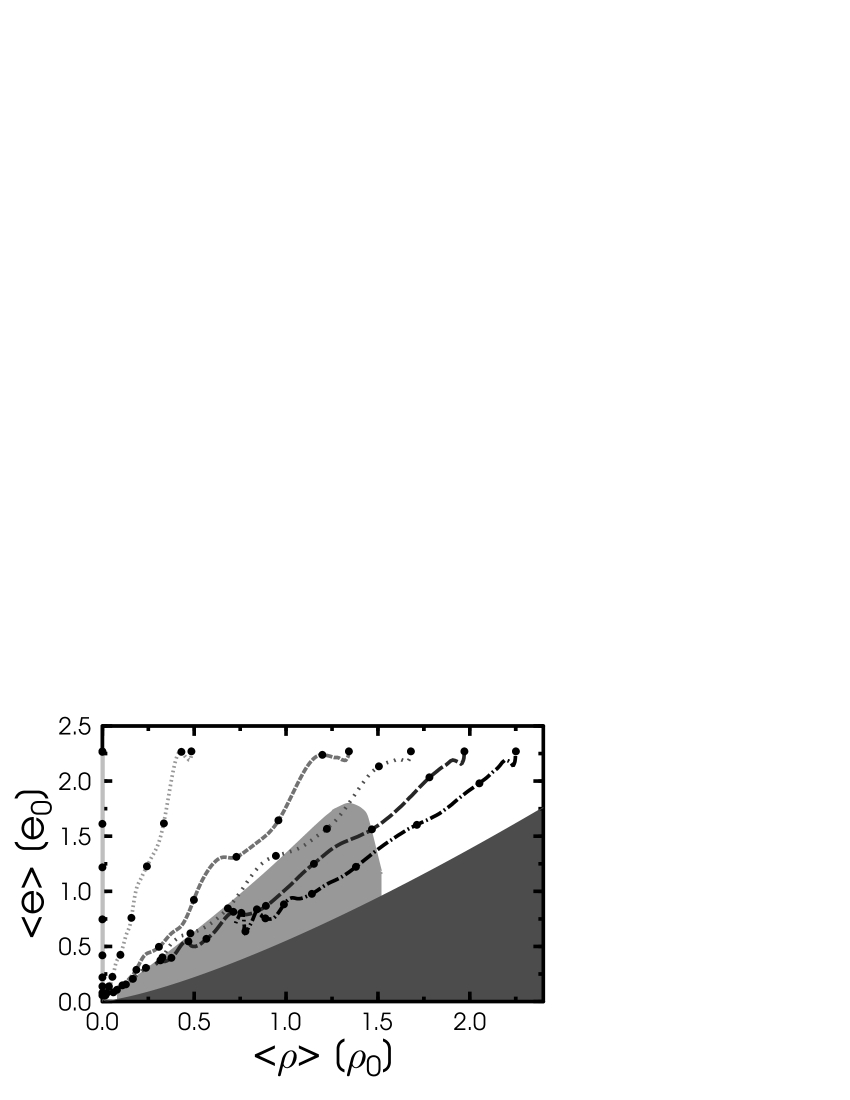
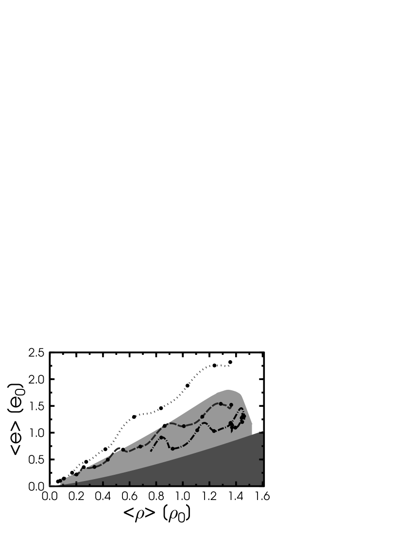
Figure 1: Evolution of the average fluid energy and baryon density through a crossover, and a weak and strong first order transition, respectively, for initial conditions I (top) and II (bottom). The densities are measured in units of nuclear matter saturation density $\rho_{0}\approx 0.16$ fm^-3, $e_{0}=m_{N}\rho_{0}\approx 0.15$ GeV/fm³, with $m_{N}\approx 0.922$ GeV the mass of a nucleon bound in infinite matter. The fat dots indicate time intervals of $\approx 1.5$ fm/c. The phase coexistence region is shaded in grey; the dark area depicts the thermodynamically forbidden region where $e<\mu_{B}\rho-p$.

Fig. 1 shows the trajectory of the system within the phase diagram for both sets of initial conditions. For simplicity, we chose a foliation of space-time by flat hypersurfaces without extrinsic curvature (i.e. surfaces of constant CM-time). The average energy density of the quark fluid on such surfaces is then given by

$$\langle{e}\rangle(t)=\frac{\int{\rm d}\sigma_{\mu}T^{\mu 0}_{\rm fluid}\,u_{\sigma}u_{\nu}T^{\sigma\nu}_{\rm fluid}}{\int{\rm d}\sigma_{\mu}T^{\mu 0}_{\rm fluid}}=\frac{\int{\rm d}^{3}x\;T^{00}_{\rm fluid}\,{e}}{\int{\rm d}^{3}x\;T^{00}_{\rm fluid}}~{},$$ (9)

and similarly for $\langle\rho\rangle$. We also average over several initial field configurations picked according to (8).

The initial condition with $\mu_{0}<\mu_{E}$ evolves smoothly through a crossover. For the other intitial conditions, the system enters the region corresponding to phase coexistence in the equilibrium phase diagram and so undergoes a first order phase transition. The explicit treatment of the dynamics of the chiral fields (in the classical approximation) in space-time allows for non-equilibrium effects and formation of inhomogeneities.

Next, we determine the RMS fluctuation of the fluid density, $\Delta\rho$, induced by the propagation of the Gaussian initial field fluctuations (8) through the phase transition. First, we determine the underlying smooth density profile on each $t={\rm const.}$ time slice by averaging over the surface of a sphere with thickness $\Delta r\simeq 1$ fm,

$$\langle\rho\rangle(t,r)={\cal N}^{-1}\int{\rm d}^{3}x\;\Theta(r+\Delta r-|\vec{x}|)\;\Theta(|\vec{x}|-r)\;\rho(t,\vec{x})~{},$$ (10)

with ${\cal N}=4\pi(\Delta r\;r^{2}+\Delta r^{\;2}\;r+\Delta r^{\;3}/3)$. This profile is determined for each initial field configuration individually. While averaging $\langle\rho\rangle(t,r)$ over “events” (i.e. initial field configurations), too, would lead to seemingly larger $\Delta e$ and $\Delta\rho$, we are interested here in density perturbations on scales of order 1 fm within individual events.

On each time slice, we then define $\Delta\rho$ as the RMS deviation from this coarse-grained density profile,

$$\Delta{\rho}^{\;2}(t)=\frac{\int{\rm d}^{3}x\left[\rho(t,\vec{x})-\langle\rho\rangle(t,r)\right]^{2}\cdot\langle{e}\rangle(t,r)}{\int{\rm d}^{3}x\;\langle{e}\rangle(t,r)~{}.}$$ (11)

We have chosen $\langle{e}\rangle(t,r)$, which is obtained in a similar way as $\langle{\rho}\rangle(t,r)$ defined in (10), as a weight in the integral to put more emphasis on the dense regions. Weighting with $\langle{\rho}\rangle(t,r)$ instead leads to qualitatively similar results.

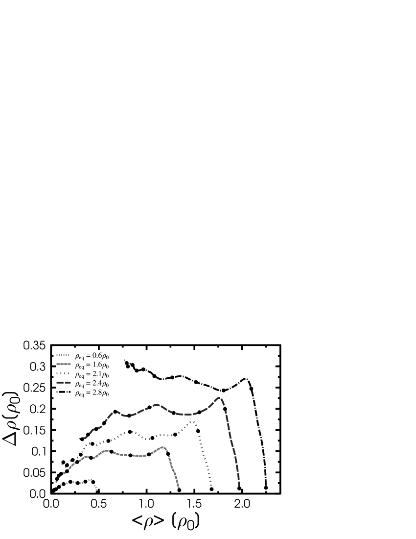
Figure 2: RMS fluctuations of the baryon density with initial condition set (I) for crossover (narrow-dots, short-dashes), weak (wide-dots, long-dashes) and strong (dash-dots) first order transitions as a function of the average baryon density. The fat dots indicate time intervals of $\approx 1.5$ fm/c.

The time evolution of the baryon density inhomogeneities for initial condition set (I) is shown in fig. 2. We start with fluctuations of the order parameter field only, so that initially $\Delta e=\Delta{\rho}=0$; this is to show the minimal degree of inhomogeneity induced just by the transition to the symmetry broken state. As the evolution progresses, the fluctuations of the order parameter field rapidly lead to density inhomogeneities in the quark fluid.

One observes that the baryon density inhomogeneities are sensitive to the dynamical evolution. The energy density inhomogeneities in this model are smaller and show a weaker dependence on the initial baryon density and are therefore not shown here.

For large initial baryon density the expansion proceeds through the region of first-order phase transitions. Here, the effective potential exhibits two local minima within the “phase coexistence” region of the equilibrium phase diagram (see e.g. fig. 1 in Paech:2003fe or figs. 2-4 in SMMR ) and so in some region of space the order parameter can be “trapped” in the symmetric phase until reaching the spinodal instability ove . This effect is more pronounced the stronger the first-order phase transition, i.e. the smaller the entropy per baryon. Consequently, density perturbations can only wash out after the double-minimum structure of the effective potential has disappeared and the order parameter “rolls down” to its new vacuum. There is therefore reasonable hope that these inhomogeneities created during the non-equilibrium phase transition are present in the final state, contrary to those from the initial state. However, even for a crossover substantial inhomogeneities could be present in the final state if they “freeze” shortly after passing the point where $V_{\rm eff}$ is flattest (or where the chiral susceptibility peaks, respectively).

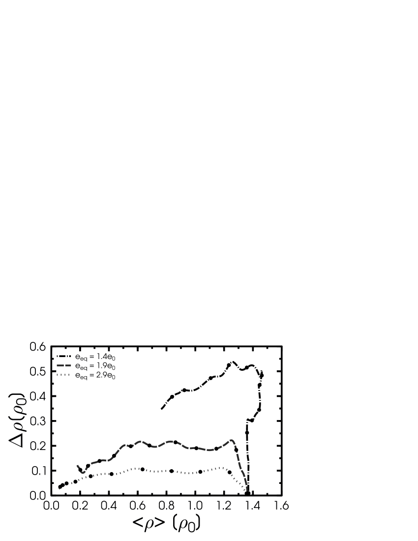
Figure 3: RMS fluctuations of the baryon density with initial condition set (II) for crossover (dots), weak (dashes) and strong (dash-dots) first order transition as a function of the average baryon density. The fat dots indicate time intervals of $\approx 1.5$ fm/c.

Fig 3 shows our results for the set (II) of initial conditions, corresponding to fixed initial baryon density $\rho_{\rm eq}=1.7\rho_{0}$ but different initial energy density $e_{\rm eq}$. Again, the amplitude of the density contrast is substantialy larger for a strong first order transition ($e_{\rm eq}=1.4e_{0}$) than for a crossover ($e_{\rm eq}=2.9e_{0}$).

IV Discussion

We have shown that the non-equilibrium dynamics of the order parameter field in heavy ion collisions can lead to large density inhomogeneities on the order of $\Delta\rho/\rho_{0}\sim 0.1-1$. Further, that the amplitude of the fluctuations depends on the structure of the effective potential: the effect is stronger for a first-order phase transition than for a crossover.

What kind of experimental signatures could arise? By analogy to inhomogeneous Big Bang nucleosynthesis ibbn , which indeed is sensitive to fluctuations of the baryon to photon ratio, one might expect that the relative hadron abundances in heavy ion collisions are modified, too. This is because the densities of various hadron species depend non-linearly on the energy- and baryon density of the hadron fluid and so fluctuations do not average out.

The present model is too schematic to allow for quantitative predictions of particle production. Nevertheless, experimental data for relative hadron multiplicities could be analyzed, for example, within the following simple model for an inhomogeneous decoupling surface to test for the presence of (energy-) density inhomogeneities. Thermal model fits to measured particle abundances are commonly performed within the grand canonical ensemble, where the density of any hadron species $i$ can be expressed in terms of the temperature $T$ and the baryon-chemical potential $\mu_{B}$. Usually, a uniform temperature and baryon-chemical potential is assumed chem_fits . On the other hand, to test for inhomogeneities, $T$ and $\mu_{B}$ could be taken as Gaussian random variables. The average density of species $i\in\left\{\pi,K,N,...\right\}$ is then given by

$$\overline{\rho_{i}}\;(\overline{T},\overline{\mu}_{B},\Delta T,\Delta\mu_{B}) = \int\limits_{0}^{\infty}dT\;P(T;\overline{T},\Delta T)$$ (12)

$$\times\int\limits_{-\infty}^{\infty}d\mu_{B}\;P(\mu_{B};\overline{\mu}_{B},\Delta\mu_{B})~{}\rho_{i}(T,\mu_{B})~{},$$

with $\rho_{i}(T,\mu_{B})$ the actual “local” density of species $i$ on the decoupling surface and

$$P(x;\overline{x},\Delta x)\sim\exp~{}-\frac{\left(x-\overline{x}\right)^{2}}{2\;\Delta x^{2}}$$ (13)

the distribution of temperatures and chemical potentials. The essential point is that $\overline{\rho_{i}}\;(\overline{T},\overline{\mu}_{B},\Delta T,\Delta\mu_{B})\neq\rho_{i}(\overline{T},\overline{\mu}_{B})$ if $\Delta T$, $\Delta\mu_{B}\neq 0$. The main contribution to the integrals in (12) is not from $\overline{T}$ and $\overline{\mu}_{B}$ but from the stationary point of the integrand. For rare and heavy particles, where quantum-statistical and relativistic effects can be neglected, there is an exponential enhancement of the density with $(\Delta\mu_{B}/\overline{T})^{2}$ and $(\Delta T/\overline{T})^{2}$; this can be shown by a saddle-point integration of (12) DPZinprep .

From our results presented in the previous section we expect that $\Delta T$, $\Delta\mu_{B}$ should be significantly larger than zero if decoupling occurs close to the first-order phase transition boundary. They should be smaller, perhaps nearly zero, when the dynamical trajectory did not cross the phase transition line. Hadron abundances at RHIC and SPS energies could be studied within such a model to search for the presence of inhomogeneities and to analyze their energy dependence detlef . In fact, central $Au+Au$ collisions at top AGS energy produce relatively cool but very baryon-dense matter HS and could also probe the phase transition line AGS_pt . Other observables should also exhibit some sensitivity to inhomogeneities, e.g. Hanbury-Brown–Twiss correlations for pions Socolowski:2004hw or production cross sections for light (anti-) nuclei, formed by coalescence of (anti-) nucleons yoffe .

References

- (1) M. Gyulassy and L. McLerran, arXiv:nucl-th/0405013; H. Stöcker, arXiv:nucl-th/0406018.
- (2) Z. Fodor and S. D. Katz, JHEP 0404 (2004) 050.
- (3) M. Stephanov, K. Rajagopal and E. V. Shuryak, Phys. Rev. Lett. 81, (1998) 4816.
- (4) C.L. Bennett et al., ApJS 148 (2003) 1; H.V. Peiris et al., ApJS 148 (2003) 213.
- (5) M. Bleicher et al., Nucl. Phys. A 638 (1998) 391.
- (6) M. Gyulassy, D. H. Rischke and B. Zhang, Nucl. Phys. A 613 (1997) 397.
- (7) For recent reviews see P. Huovinen, arXiv:nucl-th/0305064; P. F. Kolb and U. Heinz, arXiv:nucl-th/0305084.
- (8) H. J. Drescher, S. Ostapchenko, T. Pierog and K. Werner, Phys. Rev. C 65 (2002) 054902.
- (9) O. J. Socolowski, F. Grassi, Y. Hama and T. Kodama, Phys. Rev. Lett. 93 (2004) 182301.
- (10) Refs. Bleicher:wd ; GyRiZ ; Drescher:2000ec ; Socolowski:2004hw employ Glauber-like models to estimate fluctuations in the number of participants and the number of collisions. The positions of the nucleons within each nucleus are usually picked at random according to a Woods-Saxon distribution. The amplitude of energy and baryon density fluctuations in coordinate space after the two nuclei have passed through each other will be sensitive also to many-body correlations and so may require a rather careful modeling of the ground states of the colliding nuclei: G. Baym, B. Blattel, L. L. Frankfurt, H. Heiselberg and M. Strikman, Phys. Rev. C 52 (1995) 1604.
- (11) L. Bot and J. Aichelin, J. Phys. G 23 (1997) 1947.
- (12) K. Paech, H. Stöcker and A. Dumitru, Phys. Rev. C 68 (2003) 044907
- (13) M. Gell-Mann and M. Levy, Nuovo Cim. 16 (1960) 705.
- (14) O. Scavenius, A. Mocsy, I. N. Mishustin and D. H. Rischke, Phys. Rev. C 64 (2001) 045202.
- (15) O. Scavenius et al., Phys. Rev. Lett. 83 (1999) 4697; Phys. Rev. D 63 (2001) 116003.
- (16) M. A. Stephanov, Prog. Theor. Phys. Suppl. 153 (2004) 139.
- (17) F. Karsch, K. Redlich and A. Tawfik, Eur. Phys. J. C 29 (2003) 549; D. Zschiesche, G. Zeeb, S. Schramm and H. Stöcker, arXiv:nucl-th/0407117.
- (18) P. N. Meisinger and M. C. Ogilvie, Phys. Lett. B 379 (1996) 163; P. N. Meisinger, T. R. Miller and M. C. Ogilvie, Nucl. Phys. Proc. Suppl. 119 (2003) 511; A. Mocsy, F. Sannino and K. Tuominen, Phys. Rev. Lett. 92 (2004) 182302; JHEP 0403 (2004) 044; E. Megias, E. Ruiz Arriola and L. L. Salcedo, arXiv:hep-ph/0412308; see also A. Dumitru and R. D. Pisarski, Phys. Lett. B 504 (2001) 282; Phys. Lett. B 525 (2002) 95; O. Scavenius, A. Dumitru and A. D. Jackson, Phys. Rev. Lett. 87 (2001) 182302; A. Dumitru, Y. Hatta, J. Lenaghan, K. Orginos and R. D. Pisarski, Phys. Rev. D 70 (2004) 034511; A. Dumitru, J. Lenaghan and R. D. Pisarski, arXiv:hep-ph/0410294.
- (19) C. Greiner and B. Müller, Phys. Rev. D 55 (1997) 1026; A. Mocsy, Phys. Rev. D 66 (2002) 056010.
- (20) J. Ignatius, K. Kajantie, H. Kurki-Suonio and M. Laine, Phys. Rev. D 49 (1994) 3854; T. S. Biro and C. Greiner, Phys. Rev. Lett. 79 (1997) 3138; Z. Xu and C. Greiner, Phys. Rev. D 62 (2000) 036012; E. S. Fraga and G. Krein, arXiv:hep-ph/0412312.
- (21) I. N. Mishustin, J. A. Pedersen and O. Scavenius, Heavy Ion Phys. 5 (1997) 377; I. N. Mishustin and O. Scavenius, Phys. Rev. Lett. 83 (1999) 3134.
- (22) J. H. Applegate, C. J. Hogan and R. J. Scherrer, Phys. Rev. D 35 (1987) 1151; G. M. Fuller, G. J. Mathews and C. R. Alcock, Phys. Rev. D 37 (1988) 1380; K. Kainulainen, H. Kurki-Suonio and E. Sihvola, Phys. Rev. D 59 (1999) 083505.
- (23) for a review see P. Braun-Munzinger, K. Redlich and J. Stachel, arXiv:nucl-th/0304013 and references therein.
- (24) A. Dumitru, L. Portugal and D. Zschiesche, in preparation.
- (25) A. Dumitru, L. Portugal and D. Zschiesche, arXiv:nucl-th/0502051; D. Zschiesche, arXiv:nucl-th/0505054.
- (26) H. Stöcker et al., Nucl. Phys. A 566 (1994) 15c; Nucl. Phys. A 590 (1995) 271c; J. Brachmann et al., Phys. Rev. C 61 (2000) 024909; Eur. Phys. J. A 8 (2000) 549.
- (27) J. I. Kapusta, A. P. Vischer and R. Venugopalan, Phys. Rev. C 51 (1995) 901; J. Letessier, J. Rafelski, G. Torrieri, nucl-th/0411047; E. L. Bratkovskaya, S. Soff, H. Stöcker, M. van Leeuwen and W. Cassing, Phys. Rev. Lett. 92 (2004) 032302.
- (28) see e.g. eq. (30) in B. L. Ioffe, I. A. Shushpanov and K. N. Zyablyuk, Int. J. Mod. Phys. E 13 (2004) 1157;