Relativistic Harmonic Oscillator with Spin Symmetry

Abstract

The eigenfunctions and eigenenergies for a Dirac Hamiltonian with equal scalar and vector harmonic oscillator potentials are derived. Equal scalar and vector potentials may be applicable to the spectrum of an antinucleion imbedded in a nucleus. Triaxial, axially deformed, and spherical oscillator potentials are considered. The spectrum has a spin symmetry for all cases and, for the spherical harmonic oscillator potential, a higher symmetry analogous to the SU(3) symmetry of the non-relativistic harmonic oscillator is discussed.

I Introduction

Recent theoretical investigations have suggested the possibility that the lifetime of an antinucleon inside of a nucleus could be significantly enhanced thomas . The relativistic mean fields of antinucleons calculated in a self consistent Hartree approximation of a nuclear field theory dirk ; rein indicate that the scalar $V_{S}(\vec{r})$ and vector potentials $V_{V}(\vec{r})$ are approximately equal. This implies that the antinucleon spectrum will have an approximate spin symmetry tassie ; bell . This conclusion is consistent with the fact that the nucleon spectrum has an approximate pseudospin symmetry gino ; ami because the scalar and vector mean field potentials of a nucleon are approximately equal but opposite in sign and the vector potential changes sign under charge conjugation gino1 . In fact, the negative energy states of the nucleon do show a strong spin symmetry meng . Of course, whether such states could be observable can only be reliably estimated if the antinucleon annihilation potential is included in the mean field calculations.

In this paper we shall solve for the eigenfunctions and eigenenergies of the triaxial, axially deformed, and spherical relativistic harmonic oscillator for equal scalar and vector potentials with the expectation that these results could be helpful in drawing conclusions about the feasibility of observing the spectrum of an antinucleon in a nuclear environment. The spherical relativistic harmonic oscillator with spin symmetry rav ; bahdri ; tegen ; cent ; kukulin ; chao and pseudospin symmetry chen ; manuel have been studied previously, but in this paper we derive the eigenfunctions and eigenenergies for the triaxial and axially deformed harmonic oscillator as well.

II The Dirac Hamiltonian and Spin Symmetry

The Dirac Hamiltonian, $H$, with an external scalar, $V_{S}(\vec{r})$, and vector, $V_{V}(\vec{r})$, potential is given by:

$$H=\mbox{\boldmath$\alpha\cdot p$}+\beta(M+V_{S}(\vec{r}))+V_{V}(\vec{r}))~{},$$ (1)

where $\alpha$, $\beta$ are the usual Dirac matrices, $M$ is the nucleon mass and we set $c$ = 1. The Dirac Hamiltonian is invariant under a $SU(2)$ algebra for two limits: $V_{S}(\vec{r})=V_{V}(\vec{r})+C_{s}$ and $V_{S}(\vec{r})=-V_{V}(\vec{r})+C_{ps}$ where $C_{s},C_{ps}$ are constants bell . The former limit has application to the spectrum of mesons for which the spin-orbit splitting is small page and for the spectrum of an antinucleon in the mean field of nucleons gino1 ; meng . The latter limit leads to pseudospin symmetry in nuclei gino . This symmetry occurs independent of the shape of the nucleus: spherical, axial deformed, or triaxial.

II.1 Spin Symmetry Generators

The generators for the spin $SU(2)$ algebra, ${{S}}_{q}$, which commute with the Dirac Hamiltonian, $[\,H_{s}\,,\,{{S}}_{q}\,]=0$, for the spin symmetry limit $V_{S}(\vec{r})=V_{V}(\vec{r})+C_{s}$ , are given by bell

$${{{S}}}_{q}=\left(\begin{array}[]{cc}{s}_{q}&0\\ 0&{{\tilde{s}}}_{q}\end{array}\right)=\left(\begin{array}[]{cc}{s}_{q}&0\\ 0&U_{p}\,{s}_{q}\,U_{p}\end{array}\right)$$ (6)

where ${s}_{q}=\sigma_{q}/2$ are the usual spin generators, $\sigma_{q}$ the Pauli matrices, and $U_{p}=\,{\mbox{\boldmath$\sigma\cdot p$}\over p}$ is the momentum-helicity unitary operator draayer . Thus the operators ${S}_{i}$ generate an SU(2) invariant symmetry of $H_{s}$. Therefore each eigenstate of the Dirac Hamiltonian has a partner with the same energy,

$$H_{s}\ \Phi_{k,{\mu}}^{s}({\vec{r}})=E_{k}\Phi_{k,{\mu}}^{s}({\vec{r}})$$ (7)

where $k$ are the other quantum numbers and ${\mu}=\pm{1\over 2}$ is the eigenvalue of ${S}_{z}$,

$${S}_{z}\ \Phi_{k,{\mu}}^{s}({\vec{r}})={\mu}\ \Phi_{k,{\mu}}^{s}({\vec{r}}).$$ (8)

The eigenstates in the doublet will be connected by the generators ${S}_{\pm 1}$,

$${S}_{\pm}\ \Phi_{k,{\mu}}^{s}({\vec{r}})=\sqrt{{\left({1\over 2}\mp{\tilde{\mu}}\right)({3\over 2}\pm{\tilde{\mu}})}}\ \Phi_{k,{\mu}\pm 1}^{s}({\vec{r}}).$$ (9)

The fact that Dirac eigenfunctions belong to the spinor representation of the spin SU(2), as given in Eqs. (8) - (9), leads to conditions on the Dirac amplitudes mad ; ami1 ; gino2 ; witek .

II.2 Dirac Eigenfunctions and Spin Symmetry

The Dirac egenfunction can be written as a four dimensional vector

$$\Phi_{k,\mu}({\vec{r}})=\left(\begin{array}[]{c}g^{+}_{k,\mu}({\vec{r}})\\ g^{-}_{k,\mu}({\vec{r}})\\ if^{+}_{k,\mu}({\vec{r}})\\ if^{-}_{k,\mu}({\vec{r}})\end{array}\right),$$ (10)

where $g^{\pm}_{k,\mu}({\vec{r}})$ are the “upper Dirac components” where $+$ indicates spin up and $-$ spin down and $f^{\pm}_{k,\mu}({\vec{r}})$ are the “lower Dirac components” where $+$ indicates spin up and $-$ spin down. However spin symmetry imposes conditions on these eigenfunctions gino2 ; witek which are derived from Equations (8) - (9)

$$g^{+}_{k,{1\over 2}}({\vec{r}})=g^{-}_{k,-{1\over 2}}({\vec{r}})=g_{k}({\vec{r}}),$$ (11)

$$g^{+}_{k,-{1\over 2}}({\vec{r}})=g^{-}_{k,{1\over 2}}({\vec{r}})=0,$$ (12)

$${f}^{+}_{k,{1\over 2}}({\vec{r}})=-{f}^{-}_{k,-{1\over 2}}({\vec{r}})={f}_{k}({\vec{r}}),$$ (13)

$$({\partial\over\partial x}+i{\partial\over\partial x})\ {f}^{+}_{k,-{1\over 2}}({\vec{r}})=({\partial\over\partial x}-i{\partial\over\partial x})\ f^{-}_{k,{1\over 2}}({\vec{r}}),$$ (14)

$$\ {\partial\over\partial z}\ {f}^{\pm}_{k,\mp{1\over 2}}({\vec{r}})=\pm({\partial\over\partial x}\mp i{\partial\over\partial x})\ f^{\pm}_{k,\pm{1\over 2}}({\vec{r}}).$$ (15)

Thus for spin symmetry the Dirac spin doublets are

$$\Phi^{s}_{k,{1\over 2}}({\vec{r}})=\left(\begin{array}[]{c}g_{k}({\vec{r}})\\ 0\\ if_{k}({\vec{r}})\\ if^{-}_{k,{1\over 2}}({\vec{r}})\end{array}\right),\ \Phi^{s}_{k,-{1\over 2}}({\vec{r}})=\left(\begin{array}[]{c}0\\ g_{k}({\vec{r}})\\ if^{+}_{k,-{1\over 2}}({\vec{r}})\\ -if_{k}({\vec{r}}))\end{array}\right).$$ (24)

II.3 Second Order Differential Equation for the Eigenfunctions

The Dirac Hamiltonian, (1), gives first order differential relations between ${g}_{k}({\vec{r}})$ and ${f}_{k}({\vec{r}})$ and ${f}^{\pm}_{k,\mp{1\over 2}}({\vec{r}})$. In the usual way we turn these equations into a second order differential relation for the upper component. In the limit of spin symmetry this second order equation becomes

$$\left[p^{2}+2\ ({\tilde{E}}_{k}+{\tilde{M}})\ V(\vec{r})-{\tilde{E}}_{k}^{2}+{\tilde{M}}^{2}\right]{g}_{k}({\vec{r}})=0$$ (25)

where $V_{S}(\vec{r})={V(\vec{r})}+V_{S}^{0}$, $V_{V}(\vec{r})={V(\vec{r})}+V_{V}^{0}$, ${\tilde{M}}=M+V_{S}^{0}$, and ${\tilde{E}}_{k}=E_{k}-V_{V}^{0}$. From (1) and setting $\hbar$= 1, the lower components become

$$f_{k}(\vec{r})={-1\over({\tilde{M}}+{\tilde{E}})}\ {\partial\over\partial z}\ g_{k}(\vec{r}),$$ (26)

$$f_{k,\mp{1\over 2}}^{\pm}(\vec{r})={-1\over({\tilde{M}}+{\tilde{E}})}\ ({\partial\over\partial x}\mp i\ {\partial\over\partial y})\ g_{k}(\vec{r}).$$ (27)

These relations are consistent with the conditions on the eigenfunctions imposed by spin symmetry in Equations (II.2).

Equation (25) is basically the energy-dependent Schrödinger equation without any spin dependence. Hence any potential, which can be solved analytically with the non-relativistic Schroedinger equation, is solvable in the spin limit, but the energy spectrum will be different because of the nonlinear dependence on the energy. Hence the Coulomb and harmonic oscillator are solvable. The Coulomb potential has been solved (for general scalar and vector potentials) gino and applied to meson spectroscopy page . More appropriate for nuclei is the harmonic oscillator.

III Harmonic Oscillator

First we shall discuss the triaxial harmonic oscillator, then the axially symmetric harmonic oscillator, and finally the spherical harmonic oscillator.

III.1 Triaxial Harmonic Oscillator

For the potential $V(\vec{r})={{\tilde{M}}\over 2}(\omega_{1}^{2}\ x^{2}+\omega_{2}^{2}\ y^{2}+\omega_{3}^{2}\ z^{2})$, the second order differential equation (25) becomes

$$\left[{{\partial}^{2}\over{\partial x^{2}}}+{{\partial}^{2}\over{\partial y^{2}}}+{{\partial}^{2}\over{\partial z^{2}}}-{({\tilde{E}}_{n_{1},n_{2},n_{3}}+{\tilde{M}})\ {\tilde{M}}}(\omega_{1}^{2}\ x^{2}+\omega_{2}^{2}\ y^{2}+\omega_{3}^{2}\ z^{2})+{\tilde{E}}_{n_{1},n_{2},n_{3}}^{2}-{\tilde{M}}^{2}\right]{g}_{{n_{1},n_{2},n_{3}}}({\vec{r}})=0.$$ (28)

III.1.1 Eigenfunctions

Introducing the product ansatz for the eigenfunction ${g}_{{n_{1},n_{2},n_{3}}}({\vec{r}})\propto{g}_{n_{1}}({x})\ {g}_{n_{2}}({y})\ {g}_{n_{3}}({z})$, we derive the three equations

$$\left[{{\partial}^{2}\over{\partial x_{i}^{2}}}-x_{i}^{2}+2n_{i}+1\right]\ {g}_{n_{i}}({x_{i}})=0,$$ (29)

where $x_{1}=\lambda_{1}\ x,\ x_{2}=\lambda_{2}\ y,\ x_{3}=\lambda_{3}\ z,$ and

$$\lambda_{i}=\left[{({\tilde{E}}_{n_{1},n_{2},n_{3}}+{\tilde{M}})\ {\tilde{M}}\ \omega_{i}^{2}}\right]^{1\over 4},$$ (30)

$${\tilde{E}}_{n_{1},n_{2},n_{3}}^{2}-{\tilde{M}}^{2}=2\ \sum_{i}\lambda_{i}^{2}\ (n_{i}+{1\over 2})$$ (31)

The bound eigenstates are given by

$${g}_{{n_{1},n_{2},n_{3}}}({\vec{r}})={\cal N}(E_{n_{1},n_{2},n_{3}})\ {g}_{{n_{1}}}(x_{1})\ {g}_{{n_{2}}}(x_{2})\ {g}_{{n_{3}}}(x_{3}),$$ (32)

where

$${g}_{{n}}({x}_{i})=\sqrt{\lambda_{i}\over\sqrt{\pi}\ 2^{n_{i}}\ n_{i}!}\ e^{-x_{i}^{2}\over 2}\ H_{n_{i}}(x_{i}),$$ (33)

and $H_{n_{i}}(x_{i})$ is the Hermite polynomial which means that ${g}_{{n_{1},n_{2},n_{3}}}({\vec{r}})$ has $n_{1},n_{2},n_{3}$ nodes in the $x,y,$ and $z$ directions, respectively. ${\cal N}(E_{n_{1},n_{2},n_{3}})$ is the normalization determined by $\int_{-\infty}^{\infty}dx\int_{-\infty}^{\infty}dy\int_{-\infty}^{\infty}dz\ (|{g}_{{n_{1},n_{2},n_{3}}}({\vec{r}})|^{2}+|{f}^{+}_{{n_{1},n_{2},n_{3},\mu}}({\vec{r}})|^{2}+|{f}^{-}_{{n_{1},n_{2},n_{3},\mu}}({\vec{r}})|^{2})=1$.

From (II.3) the lower components are

$${f}_{{n_{1},n_{2},n_{3}}}({\vec{r}})={\cal N}(E_{n_{1},n_{2},n_{3}})\ {g}_{{n_{1}}}({x_{1}})\ {g}_{{n_{2}}}({x_{2}})\ f_{n_{3}+1}(x_{3}),$$ (34)

$${f}_{{n_{1},n_{2},n_{3}},\mp{1\over 2}}^{(\pm)}({\vec{r}})={\cal N}(E_{n_{1},n_{2},n_{3}})\ ({f}_{{n_{1}}+1}({x_{1}})\ {g}_{{n_{2}}}({x_{2}})\mp i\ {g}_{{n_{1}}}({x_{1}})\ {f}_{{n_{2}}+1}({x_{2}}))\ g_{n_{3}}(x_{3}),$$ (35)

where

$$f_{n_{i}+1}(x_{i})=\lambda_{i}\ \sqrt{\lambda_{i}\over\sqrt{\pi}\ 2^{n_{i}}\ n_{i}!}\ e^{-x_{i}^{2}}\ ({H_{n_{i}+1}(x_{i})\over 2}-n\ H_{n_{i}-1}(x_{i})).$$ (36)

Clearly the function $f_{n+1}(x)$ is a polynomial of order $n+1$. Evaluation for low $n$ demonstrates that it has $n+1$ nodes so we assume that it has $n+1$ nodes for all $n$. This means that ${f}_{{n_{1},n_{2},n_{3}}}({\vec{r}})$ has one more node in the $z$-direction than ${g}_{{n_{1},n_{2},n_{3}}}({\vec{r}})$ and the same number of nodes in the $x$ and $y$ directions as ${g}_{{n_{1},n_{2},n_{3}}}({\vec{r}})$. On the other hand the amplitudes ${f}_{{n_{1},n_{2},n_{3}},\mp{1\over 2}}^{(\pm)}({\vec{r}})$ have the same number of nodes in the z-direction as ${g}_{{n_{1},n_{2},n_{3}}}({\vec{r}})$.

Using these amplitudes the normalization becomes

$${\cal N}(E)=\sqrt{{2\ ({\tilde{E}}+{\tilde{M}})\over 3{\tilde{E}}+{\tilde{M}}}}\ .$$ (37)

III.1.2 Eigenenergies

From Equations (III.1.1) the eigenvalue equation is

$$\sqrt{{\cal E}_{n_{1},n_{2},n_{3}}+1}\ ({\cal E}_{n_{1},n_{2},n_{3}}-1)=\sum_{i=1}^{3}C_{i}\ (n_{i}+{1\over 2}),$$ (38)

where ${\cal E}_{n_{1},n_{2},n_{3}}={{\tilde{E}}_{n_{1},n_{2},n_{3}}\over{\tilde{M}}},C_{i}=2\ {\omega_{i}\over{\tilde{M}}}$, and $n_{i}=0,1,\dots$. Thus both the eigenfunctions and the eigenenergies are independent of spin.

This eigenvalue equation is solved on Mathematica:

$$E_{n_{1},n_{2},n_{3}}={\tilde{M}}\left[B(A_{n_{1},n_{2},n_{3}})+{1\over 3}+{4\over 9\ B(A_{n_{1},n_{2},n_{3}})}\right]+V_{V}^{0},$$ (39)

where

$$B(A_{n_{1},n_{2},n_{3}})=\left[A_{n_{1},n_{2},n_{3}}+\sqrt{A_{n_{1},n_{2},n_{3}}^{2}-{32\over 27}\over 2}\right]^{{2\over 3}},$$ (40)

and $A_{n_{1},n_{2},n_{3}}=\sum_{i=1}^{3}C_{i}\ (n_{i}+{1\over 2})$.

The eigenvalues $E_{n_{1},n_{2},n_{3}}$ are real for all values of ${n_{1},n_{2},n_{3}}$ as long as $C_{i},V^{0}_{S,V}$ are real. Although true it is not obvious because $B(A_{n_{1},n_{2},n_{3}})$ is not real for all $A_{n_{1},n_{2},n_{3}}$ real. From (40), $B(A_{n_{1},n_{2},n_{3}})$ is clearly complex for $A_{n_{1},n_{2},n_{3}}<\sqrt{32\over 27}$. However, we now show analytically that $E_{n_{1},n_{2},n_{3}}$ will still be real even if $B(A_{n_{1},n_{2},n_{3}})$ is complex as long as $|B(A_{n_{1},n_{2},n_{3}})|=2/3$.

The imaginary part of ${E}_{n_{1},n_{2},n_{3}}$ is

$$Im\ {E}_{n_{1},n_{2},n_{3}}={\left[B(A_{n_{1},n_{2},n_{3}})+{1\over 3}+{4\over 9\ B(A_{n_{1},n_{2},n_{3}})}\right]-\left[B(A_{n_{1},n_{2},n_{3}})+{1\over 3}+{4\over 9\ B(A_{n_{1},n_{2},n_{3}})}\right]^{*}\over 2i}$$ (41)

Writing $B(A_{n_{1},n_{2},n_{3}})=|B(A_{n_{1},n_{2},n_{3}})|e^{i\psi}$

$$Im\ {E}_{n_{1},n_{2},n_{3}}=\left(|B(A_{n_{1},n_{2},n_{3}})|-{4\over 9\ |B(A_{n_{1},n_{2},n_{3}})|}\right)sin\psi,$$ (42)

and therefore ${E}_{n_{1},n_{2},n_{3}}$ is real if $|B(A_{n_{1},n_{2},n_{3}})|=2/3$ independent of $\psi$. One can show numerically that $|B(A_{n_{1},n_{2},n_{3}})|=2/3$ for all $A_{n_{1},n_{2},n_{3}}$ in the range from zero to $\sqrt{{32\over 27}}$, $0\leq A_{n_{1},n_{2},n_{3}}\leq\sqrt{{32\over 27}}$. For $A_{n_{1},n_{2},n_{3}}\geq\sqrt{{32\over 27}}$, $B(A_{n_{1},n_{2},n_{3}})$ is clearly real and hence ${E}_{n_{1},n_{2},n_{3}}$ is real.

The spectrum is non-linear in contrast to the non-relativistic harmonic oscillator. However for small $A_{n_{1},n_{2},n_{3}}$

$$E_{n_{1},n_{2},n_{3}}\approx{\tilde{M}}\ (1+{A_{n_{1},n_{2},n_{3}}\over\sqrt{2}}+\cdots)+V^{0}_{V}$$ (43)

and therefore the binding energy, $E_{n_{1},n_{2},n_{3}}-{\tilde{M}}\approx\sum_{i=1}^{3}\omega_{i}\ (n_{i}+{1\over 2})+V_{V}^{0}$, in agreement with the non-relativistic harmonic oscillator. For large $A_{n_{1},n_{2},n_{3}}$ the spectrum goes as

$$E_{n_{1},n_{2},n_{3}}\approx{\tilde{M}}\ (A_{n_{1},n_{2},n_{3}}^{2\over 3}+{1\over 3}+\cdots)+V^{0}_{V},$$ (44)

which, in lowest order, agrees with the spectrum for ${\tilde{M}}\rightarrow$ 0 bahdri .

III.2 Axially Symmetric Harmonic Oscillator

For the axially symmetric harmonic oscillator $\omega_{1}=\omega_{2}=\omega_{\perp}$ and, hence, the potential depends only on $r_{\perp}$ and not the azimuthal angle $\phi$, $V(\vec{r})={{\tilde{M}}\over 2}(\omega_{\perp}^{2}\ r_{\perp}^{2}+\omega_{3}^{2}\ z^{2})$, where $x=r_{\perp}\ cos\phi,y=r_{\perp}\ sin\phi$. This independence of the potential on $\phi$ implies that the Dirac Hamiltionian is invariant under rotations about the $z$-axis, $[H_{s},L_{z}]=0$, where

$${{L_{z}}}=\left(\begin{array}[]{cc}{{\ell_{z}}}&0\\ 0&{{{\tilde{\ell}_{z}}}}\end{array}\right),$$ (45)

and ${\vec{\ell}}={\vec{r}}\times{\vec{p}}$ and and ${{\vec{\tilde{\ell}}}}=U_{p}\ {\vec{\ell}}\ U_{p}$. The Dirac eigenstates will then be an eigenfunction of $L_{z}$ and $J_{z}=L_{z}+S_{z}$.

$$L_{z}\Phi_{N,n_{3},\Lambda,\mu}^{s}({\vec{r}})=\Lambda\ \Phi_{N,n_{3},\Lambda,\mu}^{s}({\vec{r}}),$$ (46)

$$J_{z}\ \Phi_{N,n_{3},\Lambda,\mu}({\vec{r}})=\Omega\ \Phi_{N,n_{3},\Lambda,\mu}^{s}({\vec{r}}),\ \Omega=\Lambda+\mu,$$ (47)

where $N$ is the total harmonic oscillator quantum number and $n_{3}$ is the number of harmonic oscillator quanta in the $z$ direction, and are discussed in more detail below.

III.2.1 Eigenfunctions

Since the potential has no $\phi$ dependence the second order differential equation (25) separates into an equation for $x_{3}$ and an equation for $\rho$

$$\left[{{\partial}^{2}\over{\partial{x_{3}}^{2}}}-x_{3}^{2}+2n_{3}+1\right]\ {g}_{n_{3}}({x_{3}})=0,$$ (48)

$$\left[{{\partial}^{2}\over{\partial{\rho}^{2}}}+{1-4\ \Lambda^{2}\over 4\ \rho^{2}}-\rho^{2}+2\ n_{\perp}+2\right]\ \sqrt{\rho}\ {g}_{n_{\rho}}({\rho})=0,$$ (49)

(50)

where $\rho=\lambda_{\perp}\ r_{\perp},n_{\perp}=2n_{\rho}+\Lambda$, and

$$g_{N,n_{3},\Lambda}(\vec{r})=g_{n_{\rho}}(\rho)\ g_{n_{3}}(z)\ e^{i\Lambda\phi},$$ (51)

$$\ \lambda_{\perp}=\left[{({\tilde{E}}_{N,n_{3}}+{\tilde{M}})\ {\tilde{M}}\ \omega_{\perp}^{2}}\right]^{1\over 4},$$ (52)

$${\tilde{E}}_{N,n_{3}}^{2}-{\tilde{M}}^{2}=2\ (\lambda_{\perp}^{2}\ (\ n_{\perp}+1)+\lambda_{3}^{2}\ (\ n_{3}+{1\over 2})).$$ (53)

The quantum numbers $N,n_{\perp},n_{3},\Lambda$ are the “asymptotic” quantum numbers bohr , where $N=n_{\perp}+n_{3}$ is the total number of oscillator quanta, $N=0,1,\dots$, $n_{\perp}$ is the number of oscillator quanta in the $r_{\perp}$-direction, $n_{\perp}=0,1,\dots N$, $n_{3}$ is the number of oscillator quanta in the $z$-direction, $n_{3}=0,1,\dots N$, and $\Lambda$ is the angular momentum along the z-axis, $\Lambda=\pm n_{\perp},\pm(n_{\perp}-2)\dots\pm 1,0$. The upper components of the eigenstates are given by

$${g}_{N,n_{3},\Lambda}({\vec{r}})={\cal N}(E_{N,n_{3}})\ \lambda_{\rho}\sqrt{\lambda_{3}\ n_{\rho}!\over\pi\sqrt{\pi}\ 2^{n_{3}}\ (n_{\rho}+\Lambda)!\ n_{3}!}\ e^{-{(x_{3}^{2}+\rho^{2})\over 2}}\ \rho^{{\Lambda}}\ L^{(\Lambda)}_{n_{\rho}}(\rho^{2})\ e^{i\Lambda\phi}\ H_{n_{3}}(x_{3}),$$ (54)

where $L^{(\Lambda)}_{n_{\rho}}(\rho^{2})$ is the Laguerre polynomial which means that ${g}_{N,n_{3},\Lambda}({\vec{r}})$ has $n_{\rho},n_{3}$ nodes in the $r_{\perp}$ and $z$ directions, respectively. ${\cal N}(E_{N,n_{3}})$ is the normalization determined by $\int_{0}^{2\pi}d\phi\ \int_{0}^{\infty}\ r_{\perp}\ dr_{\perp}\ \int_{-\infty}^{\infty}\ dz(|{g}_{N,n_{3},\Lambda}({\vec{r}})|^{2}+|{f}^{+}_{N,n_{3},\Lambda,\mu}({\vec{r}})|^{2}+|{f}^{-}_{N,n_{3},\Lambda,\mu}({\vec{r}})|^{2})$ = 1 and is the same function as given in (37). These upper components do not depend on the orientation of the spin.

The lower components are

$${f}_{N,n_{3},\Lambda}({\vec{r}}) = -{\ {\cal N}(E_{N,n_{3},\Lambda})\over{\tilde{M}}+{\tilde{E}_{N,n_{3}}}}\ \ \lambda_{\rho}^{2}\ \sqrt{n_{\rho}!\over\pi\ (n_{\rho}+\Lambda)!\ }\ e^{-{\rho^{2}\over 2}}\ \rho^{{\Lambda}}\ L^{(\Lambda)}_{n_{\rho}}(\rho^{2})\ e^{i\Lambda\phi}\ f_{n_{3}+1}(x_{3}),$$ (55)

$${f}_{N,n_{3},\Lambda,-{1\over 2}}^{+}({\vec{r}}) = -{{{\cal N}(E_{N,n_{3}}})\over{\tilde{M}}+{\tilde{E}_{N,n_{3}}}}\ \ \lambda_{\rho}^{2}\ \sqrt{n_{\rho}!\over\pi(n_{\rho}+\Lambda)!\ }\ e^{-{\rho^{2}\over 2}}\ \rho^{{\Lambda}-1}$$ (56)

$$((n_{\rho}+1)\ L^{(\Lambda-1)}_{n_{\rho}+1}(\rho^{2})+(n_{\rho}+\Lambda)\ L^{(\Lambda-1)}_{n_{\rho}}(\rho^{2}))\ e^{i(\Lambda-1)\phi}\ g_{n_{3}}(x_{3}),$$

$$f_{N,n_{3},\Lambda,{1\over 2}}^{-}({\vec{r}}) = {{\cal N}(E_{N,n_{3}})\over{\tilde{M}}+{\tilde{E}_{N,n_{3}}}}\ \ \lambda_{\rho}^{2}\ \sqrt{n_{\rho}!\over\pi\ (n_{\rho}+\Lambda)!\ }\ e^{-{\rho^{2}\over 2}}\ \rho^{{\Lambda}+1}(L^{(\Lambda+1)}_{n_{\rho}}(\rho^{2})$$ (57)

$$+L^{(\Lambda+1)}_{n_{\rho}-1}(\rho^{2}))\ e^{i(\Lambda+1)\phi}\ g_{n_{3}}(x_{3}),$$

where $g_{n_{3}}(x_{3}),f_{n_{3}}(x_{3})$ are defined in (33) and (36). Clearly the function ${f}_{N,n_{3},\Lambda}({\vec{r}})$ has $n_{3}+1$ nodes in the $z$-direction, one more node than the upper component, but the same number of nodes in the $r_{\perp}$ direction. The amplitude ${f}_{N,n_{3},\Lambda,-{1\over 2}}^{+}({\vec{r}}))$ has the same number of nodes in the $z$ - direction as the upper component. However, it has $n_{\rho}+1$ nodes in the $r_{\perp}$-direction for low $n_{\rho}$ and we assume it has $n_{\rho}+1$ node for all $n_{\rho}$; that is, one more node in the $r_{\perp}$-direction than the upper component. On the other hand the amplitude ${f}_{N,n_{3},\Lambda,{1\over 2}}^{-}({\vec{r}})$ has the same number of nodes in the $z$-direction and the $r_{\perp}$-direction as the upper component.

III.2.2 Eigenenergies

From Equations (III.2.1) the eigenvalue equation is

$$\sqrt{{\cal E}_{N,n_{3}}+1}\ ({\cal E}_{N,n_{3}}-1)=C_{\perp}\ (n_{\perp}+1)+C_{3}\ (n_{3}+{1\over 2}),$$ (58)

where ${\cal E}_{N,n_{3}}={{\tilde{E}}_{N,n_{3}}\over{\tilde{M}}},C_{\perp}={{2}\ \omega_{\perp}\over{\tilde{M}}}$, and $n_{\rho},n_{3}=0,1,\dots$. Thus the eigenenergies not only have a degeneracy due to spin symmetry but they have an additional degeneracy in that they only depend on $N$ and $n_{3}$ and not on $\Lambda$.

The discussion about eigenergies is the same as for triaxial nuclei and the energy spectrum is given by

$$E_{N,n_{3}}={\tilde{M}}\left[B(A_{n_{\perp},n_{3}})+{1\over 3}+{4\over 9\ B(A_{n_{\perp},n_{3}})}\right]+V_{V}^{0},$$ (59)

where $A_{n_{\perp},n_{3}}=C_{\perp}\ (n_{\perp}+1)+C_{3}\ (n_{3}+{1\over 2})$.

III.3 Spherical Harmonic Oscillator

For a spherical harmonic oscillator $\omega_{i}=\omega$ and hence the potential depends only on the radial coordinate, $r=\sqrt{x^{2}+y^{2}+z^{2}}$, and is independent of the polar angle, $\theta$, $z=r\ cos(\theta)$, as well as $\phi$. The Dirac Hamiltonian will be invariant with respect to rotations about all three axes, $[L_{i},H_{s}]=0$ where

$${{\vec{L}}}=\left(\begin{array}[]{cc}{{\vec{\ell}}}&0\\ 0&{{\vec{\tilde{\ell}}}}\end{array}\right),$$ (60)

and hence invariant with respect to a $SU_{L}(2)\times SU(2)$ group where $SU_{L}(2)$ is generated by the orbital angular momentum operators $\vec{L}$. Since the total angular momentum, ${\vec{J}}={\vec{L}}+{\vec{S}}$, is also conserved, rather than using the four row basis for this eigenfunction, it is more convenient to introduce the spin function $\chi_{\mu}$ explicitly. The states that are a degenerate doublet are then the states with $j=\ell\pm{1\over 2}$ and they have the two row form gino2 :

$$\Psi^{s}_{n_{r},\ell,j,M}({\vec{r}})=\ \left(\begin{array}[]{c}g_{n_{r},\ell}(r)\ [Y^{(\ell)}(\theta,\phi)\ \chi]^{(j)}_{M}\\ if_{n_{r},\ell,j}(r)\ [Y^{(\ell_{j})}(\theta,\phi)\ \chi]^{(j)}_{M}\end{array}\right),$$ (61)

where $\ell_{j}=\ell\pm 1$ for $j=\ell\pm{1\over 2}$, $Y^{(\ell)}_{m}(\theta,\phi)$ is the spherical harmonic of order $\ell$, $n_{r}$ is the number of radial nodes of the upper amplitude, and $[Y^{(\ell)}(\theta,\phi)\ \chi]^{(j)}_{M}$ is the coupled amplitude $\sum_{m\mu}C^{\ell{1\over 2}j}_{m\mu M}Y^{(\ell)}_{m}(\theta,\phi)\ \chi_{\mu}$. Thus the spherical symmetry reduces the number of amplitudes in the doublet even further from four to three .

The Dirac eigenstates will then be an eigenfunction of ${\vec{L}}\cdot{\vec{L}}$, $\vec{J}\cdot\vec{J}$, and $J_{z}$,

$${\vec{J}}\cdot{\vec{J}}\ \Psi_{n_{r},\ell,j,M}^{s}({\vec{r}})=j\ (j+1)\ \Psi_{n_{r},\ell,j,M}^{s}({\vec{r}}),$$ (62)

$${\vec{L}}\cdot{\vec{L}}\ \Psi_{n_{r},\ell,j,M}^{s}({\vec{r}})=\ell\ (\ell+1)\ \Psi_{n_{r},\ell,j,M}^{s}({\vec{r}}),$$ (63)

$$J_{z}\ \Psi_{n_{r},\ell,j,M}^{s}({\vec{r}})=M\ \Psi_{n_{r},\ell,j,M}^{s}({\vec{r}}).$$ (64)

The differential equation for $g_{n_{r},\ell}(r)$ becomes:

$$\left[{d^{2}\over dx^{2}}-{\ell(\ell+1)\over x^{2}}-x^{2}+{{({\tilde{E}_{N}}^{2}-{\tilde{M}}^{2})}\over\left[({\tilde{E}_{N}}+{\tilde{M}})\ {{\tilde{M}}\omega^{2}\over 2}\right]^{1\over 2}}\right]\ r\ g_{n_{r},\ell}({r})=0,$$ (65)

where ${\tilde{E}_{N}}=E_{N}-V^{0}_{V},\ {\tilde{M}}=M+V^{0}_{S},\ x=\lambda\ r$, and

$$\lambda=\left[({\tilde{E}_{N}}+{\tilde{M}})\ {{\tilde{M}}\omega^{2}}\right]^{1\over 4}$$ (66)

$${\tilde{E}_{N}^{2}}-{\tilde{M}}^{2}=2\ \lambda^{2}\ (N+{3\over 2})$$ (67)

III.3.1 Eigenfunctions

The solutions to this differential equation are well known and lead to the upper amplitudes of the eigenfunctions

$${g}_{n_{r},\ell}({r})={\cal{N}}(E_{N,\ell})\ \sqrt{{2\ \lambda^{3}\ n!\over\Gamma(\ell+n+{3\over 2})}}\ e^{-{{x^{2}}\over 2}}x^{\ell}L_{n_{r}}^{(\ell+{1\over 2})}(x^{2}),$$ (68)

where ${\cal N}(E_{N})$ is the normalization determined by $\int_{0}^{2\pi}d\phi$ $\int_{-\pi}^{\pi}sin(\theta)d\theta$ $\int_{0}^{\infty}$ $r^{2}\ dr(|{g}_{n_{r},\ell}({\vec{r}})|^{2}$ $+\ |{f}_{n_{r},\ell,j}({\vec{r}})|^{2})$ = 1 and is the same function as given in (37). Clearly ${g}_{n_{r},\ell}({r})$ has $n_{r}$ nodes in the radial direction.

The lower components are

$${f}_{n_{r},\ell,j=\ell-{1\over 2}}({\vec{r}})=$$

$$-{{{\cal N}(E_{N}})\over{\tilde{M}}+{\tilde{E}_{N}}}\ \sqrt{{2\ \lambda^{5}\ n!\over\Gamma(\ell+n_{r}+{3\over 2})}}\ e^{-{{x^{2}}\over 2}}x^{\ell-1}((n_{r}+1)\ L^{(\ell-{1\over 2})}_{n_{r}+1}(x^{2})+(n_{r}+\ell+{1\over 2})\ L^{(\ell-{1\over 2})}_{n_{r}}(x^{2})),$$ (69)

$$f_{n_{r},\ell,j=\ell+{1\over 2}}({\vec{r}})=\\ {{{\cal N}(E_{N}})\over{\tilde{M}}+{\tilde{E}_{N}}}\ \sqrt{{2\ \lambda^{5}\ n!\over\Gamma(\ell+n_{r}+{3\over 2})}}\ e^{-{{x^{2}}\over 2}}x^{\ell+1}(L^{(\ell+{3\over 2})}_{n_{r}}(x^{2})+L^{(\ell+{3\over 2})}_{n_{r}-1}(x^{2}))$$ (70)

Clearly the function ${f}_{n_{r},\ell,j=\ell-{1\over 2}}({\vec{r}})$ has $n_{r}+1$ nodes, one more node than the upper component. The amplitude ${f}_{n_{r},\ell,j=\ell+{1\over 2}}({\vec{r}}))$ has the same number of nodes as the upper component. This agrees with the general theorem relating the number of radial nodes of the lower comonents to the number of radial nodes of the upper componentami2 .

III.3.2 Energy Eigenvalues

The eigenvalue equation is

$$\sqrt{{\cal E}_{N}+1}\ ({\cal E}_{N}-1)=C\ (N+{3\over 2}),$$ (71)

where ${\cal E}_{N}={{\tilde{E}}_{N}\over{\tilde{M}}},C={{2}\ \omega\over{\tilde{M}}}$, and $N$ is the total oscillator quantum number, $N=2n+\ell=0,1,\dots$. We note that there is not only a degeneracy due to spin symmetry but there is also the usual degeneracy of the non-relativistic harmonic oscillator; namely, that the energy depends only on the total harmonic oscillator quantum number and the states with orbital angular momentum $\ell=N,N-2,\dots,0$ or 1 and angular momentum projection $m=\ell,\ell-1,\dots,\ell$ are all degenerate.

Again the eigenvalue is:

$$E_{N}={\tilde{M}}\left[B(A_{N})+{1\over 3}+{4\over 9\ B(A_{N})}\right]+V_{V}^{0},$$ (72)

and $A_{N}=C(N+{3\over 2})$.

III.4 Energy Spectrum

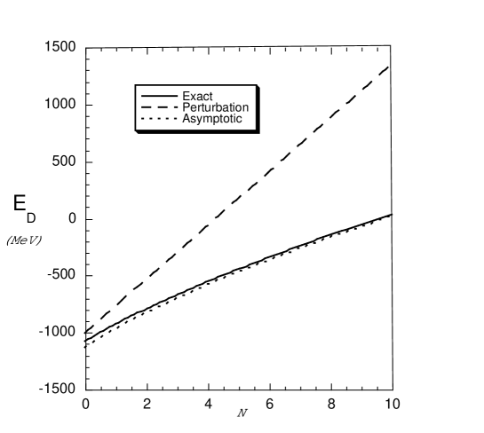
Figure 1: The Dirac binding energies, $E_{D}$, for the spherical harmonic oscillator as a function of $N$. The exact enegies are the solid line, the perturbation appoximation is the dashed line, and the asymptotic approximation is the short dashed line.

In Figure 1 we plot the spherical harmonic oscillator Dirac binding enegies $E_{D}=E_{N}-M$ with $E_{N}$ given in Eq. (72), the solid curve, as a function of $N$. We chose the parameters to fit the lowest eigenenergies of the spectrum of an anti-proton outside of ${}^{16}O$ in the relativistic mean field aprroximation thomas and they are $C=1.33,{\tilde{M}}=252$ MeV, and $V^{0}_{V}=-677$ MeV.

The dashed curve is $E_{D}$ using the pertubation approximation of $E_{N}$ given in Eq. (43). The short-dashed curve is $E_{D}$ using the asymptotic limit of $E_{N}$ given in Eq. (44). Clearly the eigenenergies are in the relativistic asymptotic regime and not the linear regime of the non-relativistic harmonic oscillator.

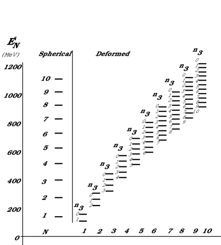
Figure 2: On the left the excitation energies, $E_{N}^{*}$, for the spherical harmonic oscillator are plotted for each $N$. Each level has a $(N+2)\ (N+1)$ degeneracy because of spin symmetry and because the allowed orbital angular momenta are $\ell=N,N-2,\dots 0$ or $1$ and the allowd orbital angular momentum projections are $m=\ell,\ell-1,\dots-\ell$. On the right the excitation energies, $E^{*}$, for the deformed harmonic oscillator are plotted in staggered groups for each $N$. Each group contains the levels for $n_{3}=0,1,\dots,N$. Each level has a $2\ (N-n_{3})+1$ degeneracy for $(N-n_{3})$ even and a $2\ (N-n_{3}+1)$ degeneracy for $(N-n_{3})$ odd because of spin symmetry and because the allowed orbital angular momentum projections are $\Lambda=\pm(N-n_{3}),\pm(N-n_{3}-2),\dots\pm 1$ or $0$.

In Figure 2 we plot the spherical harmonic oscillator excitation energies ${E}^{*}_{N}=E_{N}-E_{0}$ for different $N$ on the far left. Each level has a $(N+2)\ (N+1)$ degeneracy because of spin symmetry and because the allowed orbital angular momenta are $\ell=N,N-2,\dots 0$ or $1$ and the allowed orbital angular momentum projections are $m=\ell,\ell-1,\dots-\ell$. In the right of Figure 2 we plot the deformed excitation energies ${E}^{*}_{N,n_{3}}=E_{N,n_{3}}-E_{0,0}$. The deformed excitation energies are staggered in groups for each $N$ and each group contains the levels for $n_{3}=0,1,\dots,N$ with the excitation energy increasing with decreasing $n_{3}$. The dimensionless oscillator strengths are determined by $C^{3}=C_{\perp}^{2}\ C_{3}$ and assuming a deformation $\delta=0.33$ which leads to $C_{\perp}=1.49,C_{3}=1.05$ bohr . Each level has a $2\ (N-n_{3})+1$ degeneracy for $(N-n_{3})$ even and a $2\ (N-n_{3}+1)$ degeneracy for $(N-n_{3})$ odd because of spin symmetry and because the allowed orbital angular momentum projections are $\Lambda=\pm(N-n_{3}),\pm(N-n_{3}-2),\dots\pm 1$ or $0$. The splitting of the levels within each $N$ appears to be approximately linear with $n_{3}$.

III.5 Relativistic Contribution

The normalization ${\cal N}(E)$ has the same functional form independent on whether the harmonic oscillator is triaxial, axially deformed, or spherical. This normalization has also been calculated independently by using $\int_{-\infty}^{\infty}dx\int_{-\infty}^{\infty}dy\int_{-\infty}^{\infty}dz\ (|{f}_{\mu}^{+}({\vec{r}})|^{2}+|{f}_{\mu}^{-}({\vec{r}})|^{2})=\int_{-\infty}^{\infty}dx\int_{-\infty}^{\infty}dy\int_{-\infty}^{\infty}dz\ {g}({\vec{r}})^{*}\ {p^{2}\over({\tilde{E}}+{\tilde{M}})^{2}}\ {g}({\vec{r}})$ and we find agreement between the two different ways of calculating ${\cal N}(E)$.

This also tells us that the probability of the lower component to the upper component is given by:

$$R_{k}={\int_{-\infty}^{\infty}dx\int_{-\infty}^{\infty}dy\int_{-\infty}^{\infty}dz\ (|{f}_{k,\mu}^{+}({\vec{r}})|^{2}+|{f}_{k,\mu}^{-}({\vec{r}})|^{2})\over\int_{-\infty}^{\infty}dx\int_{-\infty}^{\infty}dy\int_{-\infty}^{\infty}dz\ |{g}_{k}({\vec{r}})|^{2}}={{\tilde{E}_{k}}-{\tilde{M}}\over 2\ ({\tilde{E}_{k}}+{\tilde{M}})}.$$ (73)

Thus for ${\tilde{E}}_{k}\approx{\tilde{M}}$ the system is not very relativistic and the contribution of the lower components is small. For ${\tilde{E}}_{k}>>{\tilde{M}}$, this ratio approaches $1\over 2$. For free particles this ratio approaches unity which indicates that the harmonic oscillator reduces the relativistic effect.

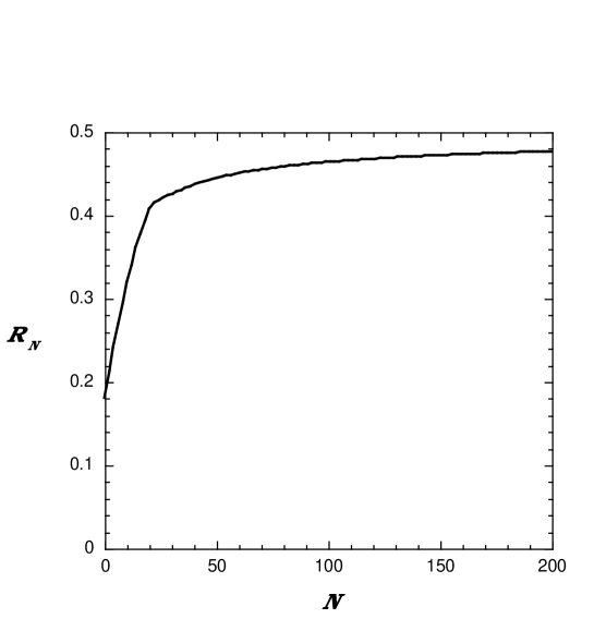
Figure 3: The ratio of the probability of the lower components to the upper components, $R_{N}$, for the spherical harmonic oscillator as a function of $N$.

In Figure 3 we plot this ratio for the spherical harmonic oscillator, $R_{N}$, as a function of $N$. Even for the most bound states this probability is about 20 % and thus the antinucleon bound inside the nucleus is much more relativistic than a nucleon inside a nucleus for which this probability is about 1 %.

IV Higher Order Symmetry

The non-relativistic spherical harmonic oscillator has an $SU(3)$ symmetry phil . This symmetry is generated by the orbital angular momentum operators ${\vec{\ell}}$ and the quadrupole operators

$${q}_{m}={[rr]_{m}^{(2)}}\lambda_{NR}^{2}+{[pp]_{m}^{(2)}\over\lambda_{NR}^{2}},$$ (74)

where ${[rr]_{m}^{(2)}}$ means coupled to angular momentum rank 2 and projection $m$ and $\lambda_{NR}=\sqrt{M\omega}$. This quadrupole operator is then a function of the dimensionless variable $\vec{x}_{NR}=\lambda_{NR}\ \vec{r}$. These generators connect the degenerate states of the harmonic oscillator.

The same degeneracy that appears in the non-relativistic spectrum appears in the relativistic spectrum. The upper component of the relativistic eigenfunction given in Eq. (61) has the same form as the non-relativistic harmonic oscillator eigenfunction except that it is a function of the relativistic dimensionless variable $\vec{x}=\lambda\vec{r}$. Therefore if the generators are written in terms of the relativistic dimesionless variable they will connect the upper components of all the degenerate states of the relativistic harmonic oscillator in the same manner as the non-relavitistic quadrupole operator in Eq. (74) connects the degenerate eigenstates of the non-relativistic harmonic oscillator. Likewise, since the lower components are proportional to $U_{p}$ operating on the upper components, the dimensionless quadrupole operator transformed by $U_{p}$ connects the lower components of the degenerate states in the same manner as the non-relavitistic quadrupole operator in Eq. (74) connects the degenerate eigenstates of the non-relativistic harmonic oscillator. However $\lambda$ depends on the energy ( see Eq. (66)) and therefore the relativistic quadrupole generator is

$${Q_{m}}=\left(\begin{array}[]{cc}{[rr]_{m}^{(2)}}&0\\ 0&{U_{p}\ [rr]_{m}^{(2)}\ U_{p}}\end{array}\right)\omega\sqrt{{\tilde{M}}(H_{s}-V_{V}^{0}+{\tilde{M}})}+[pp]_{m}^{(2)}{1\over\omega}\sqrt{{\tilde{M}}(H_{s}-V_{V}^{0}+{\tilde{M}})}$$ (75)

since $U_{p}$ commutes with $\vec{p}$. These generators along with the orbitial angular momentum, ${\vec{L}}$, given by (60), connect the degenerate states with each other. Work on the algebra is in progress. For $M\rightarrow\infty,Q_{m}\rightarrow{\bar{Q}}_{m}$,

$${\bar{Q}}_{m}=\left(\begin{array}[]{cc}{[rr]_{m}^{(2)}}&0\\ 0&{U_{p}\ [rr]_{m}^{(2)}\ U_{p}}\end{array}\right)\ {\omega\ {M}}+{[pp]_{m}^{(2)}\over\omega\ {M}}\ ,$$ (76)

which forms an $SU(3)$ algebra with ${\vec{L}}$.

V Summary and Conclusions

We have derived the eigenfunctions and eigenenergies for a Dirac Hamiltonian with triaxial, axially deformed, and spherical harmonic oscillator potentials and with equal scalar and vector potentials. In all cases the Dirac Hamiltonian is invariant with respect to the $SU(2)$ spin symmetry and thus the eigenenergies are independent of spin. For axially symmetric potentials the Dirac Hamiltonian is invariant with respect to a $SU(2)\times U(1)$ group and the eigenenergies are degenerate with respect to the orbital angular momentum projection along the $z$-axis which generates the $U(1)$. For the spherical oscillator the eigenenergies are degenerate with respect to the orbital angular mometum and hence invariant under the $SU_{L}(2)\times SU(2)$ group. These energies also have a higher degeneracy which is the same as the non-relativistic harmonic oscillator; that is, they depend only on the total harmonic oscillator quantum number. The generators that connect these degenerate states have been derived but a larger symmetry group analogous to $SU(3)$ symmetry has yet to be identified. However, for infinite mass, the spherical relativistic harmonic oscillator is invariant with respect to an $SU(3)\times SU(2)$ group.

The eigenenergies have the same functional form for triaxial, axially deformed, and spherical potentials and depend on one variable which is a linear combination of the oscillator quanta in a given direction weighted by the strength of the oscillator potential in that direction. The spectrum is infinite and the eigenenergies and are linear in the harmonic oscillator quanta for small oscillator strength but increase slower than linear for large oscillator strength.

VI Acknowledgements

The author would like to thank T. Bürvenich, R. Lisboa, M. Malheiro, A. S. de Castro, P. Alberto and M. Fiolhais for discussions. This work was supported by the U.S. Department of Energy under contract W-7405-ENG-36.

References

- (1) T. Bürvenich et al, Phys. Lett. B 542, 261 (2002).
- (2) B. D. Serot and J. D. Walecka, Adv. in Nucl. Phys. 16, 1 (1985).
- (3) P. G. Reinhard, Rep. Prog. Phys. 16, 1 (1985). Phys. Lett. B 52, 439 (1989).
- (4) G. B. Smith and L. J. Tassie, Ann. Phys. 65, 352 (1971).
- (5) J. S. Bell and H. Ruegg, Nucl. Phys. B 98, 151 (1975).
- (6) J. N. Ginocchio, Phys. Rev. Lett. 78, 436 (1997).
- (7) J. N. Ginocchio and A. Leviatan, Phys. Lett. B 425, 1 (1998).
- (8) J. N. Ginocchio, Phys. Rep. 315, 231 (1999).
- (9) S. G. Zhou, J. Meng, and P. Ring, submitted to Phys. Rev. Lett. (2003); Nucl-th/0304067.
- (10) F. Ravndal, Phys. Lett. B 113, 57 (1982).
- (11) R. K. Bhaduri, Models of the Nucleon: From quarks to Soliton, (Addison-Wesley, 1988).
- (12) R. Tegen, Ann.Phys. 197, 439 (1990).
- (13) M. Centelles, X. Vinas, M. Barranco and P. Schuck, Nucl. Phys. A 519, 73c (1990).
- (14) V. I. Kukulin, G. Loyola and M. Moshinsky, Phys. Lett. A 158, 19 (1991).
- (15) Q. W.-Chao, Chin. Phys. 11, 757 (2002).
- (16) T.-S. Chen, H.-F. Lu, J. Meng, S.-Q. Zhang, S.-G. Zhou, Chin. Phys. Lett. 20, 358 (2003).
- (17) R. Lisboa, M. Malheiro, A. S. de Castro, P. Alberto and M. Fiolhais, nucl-th/0310071.
- (18) P. R. Page, T. Goldman, and J. N. Ginocchio, Phys. Rev. Lett. 86, 204 (2001).
- (19) A. L. Blokhin, C. Bahri and J. P. Draayer, Phys. Rev. Lett. 74 (1995) 4149.
- (20) J.N. Ginocchio and D. G. Madland, Physical Review C 57, 1167 (1998).
- (21) J.N. Ginocchio and A. Leviatan, Physical Review Letters 87, 072502 (2001).
- (22) J.N. Ginocchio, Phys. Rev. C 66, 064312 (2002).
- (23) P.J. Borycki, J. Ginocchio, W. Nazarewicz, and M. Stoitsov, Phys. Rev. C 68, 014304 (2003).
- (24) A. Bohr and Ben R. Mottelson, Nuclear Structure, Vol. II (W. A. Benjamin, Reading, Ma., 1975).
- (25) A. Leviatan and J.N. Ginocchio, Physics Letters B 518 214 (2001).
- (26) J.P. Elliott, Proc. Roy. Soc. A 245 128 (1958).