Assessment of uncertainties in QRPA $0\nu\beta\beta$-decay nuclear matrix elements

Abstract

The nuclear matrix elements $M^{0\nu}$ of the neutrinoless double beta decay ($0\nu\beta\beta$) of most nuclei with known $2\nu\beta\beta$-decay rates are systematically evaluated using the Quasiparticle Random Phase Approximation (QRPA) and Renormalized QRPA (RQRPA). The experimental $2\nu\beta\beta$-decay rate is used to adjust the most relevant parameter, the strength of the particle-particle interaction. New results confirm that with such procedure the $M^{0\nu}$ values become essentially independent on the size of the single-particle basis. Furthermore, the matrix elements are shown to be also rather stable with respect to the possible quenching of the axial vector strength parametrized by reducing the coupling constant $g_{A}$, as well as to the uncertainties of parameters describing the short range nucleon correlations. Theoretical arguments in favor of the adopted way of determining the interaction parameters are presented. Furthermore, a discussion of other implicit and explicit parameters, inherent to the QRPA method, is presented. Comparison is made of the ways these factors are chosen by different authors. It is suggested that most of the spread among the published $0\nu\beta\beta$ decay nuclear matrix elements can be ascribed to these choices.

I Introduction

Inspired by the spectacular discoveries of oscillations of atmospheric fukuda98 , solar clev98 ; abdu99 ; fukuda02 ; ahmad01 , and reactor neutrinoseguchi03 (for recent reviews see McKeown04 ; Concha03 ; Grimus03 ; bil03 ; Langacker04 ) the physics community worldwide is embarking on the next challenging problem, finding whether neutrinos are indeed Majorana particles as many particle physics models suggest. Study of the neutrinoless double beta decay ($0\nu\beta\beta$) is the best potential source of information about the Majorana nature of the neutrinos FS98 ; V02 ; EV2002 ; EE04 . Moreover, the rate of the $0\nu\beta\beta$ decay, or limits on its value, can be used to constrain the neutrino mass pattern and the absolute neutrino mass scale, i.e., information not available by the study of neutrino oscillations. (The goals, and possible future directions of the field are described, e.g., in the recent study matrix . The issues particularly relevant for the program of $0\nu\beta\beta$ decay search are discussed in nustudy .)

The observation of $0\nu\beta\beta$ decay would immediately tell us that neutrinos are massive Majorana particles. But without accurate calculations of the nuclear matrix elements it will be difficult to reach quantitative conclusions about the absolute neutrino masses and mass hierarchies and confidently plan new experiments. Despite years of effort there is at present a lack of consensus among nuclear theorists how to correctly calculate the nuclear matrix elements, and how to estimate their uncertainty (see e.g. EE04 ; bah04 ). Since an overwhelming majority of published calculations is based on the Quasiparticle Random Phase Approximation (QRPA) and its modifications, it is worthwhile to try to see what causes the sizable spread of the calculated $M^{0\nu}$ values. Does it reflect some fundamental uncertainty, or is it mostly related to different choices of various adjustable parameters? If the latter is true (and we believe it is) can one find and justify an optimal choice that largely removes such unphysical dependence?

In the previous paper Rod03a we have shown that by adjusting the most important parameter, the strength of the isoscalar particle-particle force so that the known rate of the $2\nu\beta\beta$-decay is correctly reproduced, the dependence of the calculated $0\nu\beta\beta$ nuclear matrix elements $M^{0\nu}$ on other things that are not a priori fixed, is essentially removed. In particular, we have shown that this is so as far the number of single particle states included is concerned, and the choice of the different realistic representations of the nucleon $G$-matrix. In Rod03a we applied this procedure to the $0\nu\beta\beta$ decay candidate nuclei, ⁷⁶Ge, ¹⁰⁰Mo, ¹³⁰Te, and ¹³⁶Xe.

In the present work we wish to expand and better justify the ideas presented in Rod03a . First, the method is systematically applied to calculate the nuclear matrix elements $M^{0\nu}$ for most of the nuclei with known experimental $2\nu\beta\beta$-decay rates. Second, the sensitivity of the results to variation of other model parameters is tested. These are the axial vector quenching factor, commonly described as a modification of the constant $g_{A}$, and the parameters that describe the effect of the short range correlations. Finally, arguments in favor of the chosen calculation method are presented and discussed.

II Details of the calculation of $0\nu\beta\beta$ decay matrix elements

Provided that a virtual light Majorana neutrino with the effective mass $\langle m_{\beta\beta}\rangle$,

$$\langle m_{\beta\beta}\rangle=\sum_{i}^{N}|U_{ei}|^{2}e^{i\alpha_{i}}m_{i}~{},~{}({\rm all~{}}m_{i}\geq 0)~{},$$ (1)

is exchanged between the nucleons foot1 the half-life of the $0\nu\beta\beta$ decay is given by

$$\frac{1}{T_{1/2}}=G^{0\nu}(E_{0},Z)|{M^{\prime}}^{0\nu}|^{2}|\langle m_{\beta\beta}\rangle|^{2}~{},$$ (2)

where $G^{0\nu}(E_{0},Z)$ is the precisely calculable phase-space factor, and ${M^{\prime}}^{0\nu}$ is the corresponding nuclear matrix element. Thus, obviously, any uncertainty in ${M^{\prime}}^{0\nu}$ makes the value of $\langle m_{\beta\beta}\rangle$ equally uncertain.

The elements of the mixing matrix $|U_{ei}|^{2}$ and the mass-squared differences $\Delta m^{2}$ can be determined in oscillation experiments. If the existence of the $0\nu\beta\beta$ decay is proved and the value of $T_{1/2}$ is found, combining the knowledge of the first row of the neutrino mixing matrix $|U_{ei}|^{2}$ and the mass-squared differences $\Delta m^{2}$, a relatively narrow range of absolute neutrino mass scale can be determined, independently of the Majorana phases $\alpha_{i}$ in most situations EV2002 ; PP2002 . However, such an important insight is possible only if the nuclear matrix elements are accurately known.

The nuclear matrix element ${M^{\prime}}^{0\nu}$ is defined as

$${M^{\prime}}^{0\nu}=\left(\frac{g_{A}}{1.25}\right)^{2}~{}\langle f|-\frac{M^{0\nu}_{F}}{g^{2}_{A}}+M^{0\nu}_{GT}+M^{0\nu}_{T}|i\rangle$$ (3)

where $|i\rangle,~{}(|f\rangle)$ are the wave functions of the ground states of the initial (final) nuclei. We note that for $g_{A}=1.25$ nuclear matrix element ${M^{\prime}}^{0\nu}$ coincides with ${M}^{0\nu}$ of our previous work Rod03a . We have chosen this, somewhat awkward, parameterization so that we could later modify the value of $g_{A}$ and still use the same phase space factor $G^{0\nu}(E_{0},Z)$ that contains $g_{A}^{4}=(1.25)^{4}$, tabulated e.g. in Ref. si99 .

The explicit forms of the operators $M^{0\nu}_{F},M^{0\nu}_{GT}$ and $M^{0\nu}_{T}$ are given in Ref. si99 . In order to explain the notation used below we summarize here only the most relevant formulae. We begin with the effective transition operator in the momentum representation

$$\Omega=\tau^{+}\tau^{+}\frac{(-h_{F}+h_{GT}\sigma_{12}-h_{T}S_{12})}{q(q+E^{m}_{J}-(E^{i}_{g.s.}+E^{f}_{g.s})/2)}~{},~{}~{}\sigma_{12}=\vec{\sigma_{1}}\cdot\vec{\sigma_{2}}~{},~{}~{}S_{12}=3\vec{\sigma_{1}}\cdot\vec{q}\vec{\sigma_{2}}\cdot\vec{q}-\sigma_{12}~{}.$$ (4)

Here, $h_{F}(q^{2})=g_{V}^{2}(q^{2}),$ and

$$h_{GT}=g_{A}^{2}\left[1-\frac{2}{3}\frac{\vec{q}^{2}}{\vec{q}^{2}+m_{\pi}^{2}}+\frac{1}{3}\left(\frac{\vec{q}^{2}}{\vec{q}^{2}+m_{\pi}^{2}}\right)^{2}\right],h_{T}=g_{A}^{2}\left[\frac{2}{3}\frac{\vec{q}^{2}}{\vec{q}^{2}+m_{\pi}^{2}}-\frac{1}{3}\left(\frac{\vec{q}^{2}}{\vec{q}^{2}+m_{\pi}^{2}}\right)^{2}\right].$$ (5)

For simplicity we do not explicitly indicate here the $q^{2}$ dependence of the form factor $g_{A}(q^{2})$ (the usual dipole form is used for both $g_{V}(q^{2})$ and $g_{A}(q^{2})$), and the terms containing $1/m_{p}^{2}$. The full expressions can be found in Ref. si99 and are used in the numerical calculations. Note that the space part of the momentum transfer four-vector is used in Eq. (5) since the time component is much smaller than $q\equiv|\vec{q}|$.

The parts containing $\vec{q}^{2}+m_{\pi}^{2}$ come from the induced pseudoscalar form factor $g_{P}$ for which the partially conserved axial-vector current hypothesis (PCAC) has been used. In comparison with most of previous $0\nu\beta\beta$ decay studies SSPF1997 ; VZ86 ; CFT87 ; MK88 the higher order terms of the nucleon current (in particular the induced pseudoscalar as well as the weak magnetism) are included in the present calculation, resulting in a reduction of the nuclear matrix element by about 30% si99 . In the numerical calculation of ${M^{\prime}}^{0\nu}$ here the summation over the virtual states in the intermediate nucleus is explicitly performed.

The relatively important role of the induced nucleon currents deserves a comment. In the charged current neutrino induced reactions the parts of the cross section containing $g_{P}$ are usually unimportant because they appear proportional to the outgoing charged lepton mass. That comes about because the equation of motion for the outgoing on-mass-shell lepton is used. Here, this cannot be done since the neutrino is virtual, and highly off-mass-shell.

In order to calculate the matrix element in the coordinate space, one has to evaluate first the ‘neutrino potentials’ that in our case explicitly depend on the energy $E^{m}$ of the intermediate state,

$$H_{K}(r_{12})=\frac{2}{\pi g_{A}^{2}}{R}\int_{0}^{\infty}~{}f_{K}(qr_{12})~{}\frac{h_{K}(q^{2})qdq}{q+E^{m}-(E_{i}+E_{f})/2}~{},$$ (6)

where $K$ stands for $F,GT,T$. $f_{F,GT}(qr_{12})=j_{0}(qr_{12})$ and $f_{T}(qr_{12})=-j_{2}(qr_{12})$, where $j_{0,2}$ are the spherical Bessel functions. The form factor combinations $h_{K}$ are defined in  Eq.(5), $r_{12}$ is the distance between the nucleons, $R$ is the nuclear radius, and $E_{i}(E_{f})$ are the ground state energies of the initial (final) nuclei. We note that in Ref. si99 the tensor potential is presented incorrectly with the spherical Bessel function $j_{0}(x)=\sin(x)/x$ instead of $j_{2}(x)$. However, the numerical results were obtained with the correct expression.

The individual parts of the matrix element ${M^{\prime}}^{0\nu}$, Eq.(3), are given by the expression:

$$M_{K}= \sum_{J^{\pi},k_{i},k_{f},\mathcal{J}}\sum_{pnp^{\prime}n^{\prime}}(-1)^{j_{n}+j_{p^{\prime}}+J+{\mathcal{J}}}\sqrt{2{\mathcal{J}}+1}\left\{\begin{array}[]{c c c}j_{p}&j_{n}&J\\ j_{n^{\prime}}&j_{p^{\prime}}&{\mathcal{J}}\end{array}\right\}$$ (10)

$$\langle p(1),p^{\prime}(2);{\mathcal{J}}\parallel f(r_{12})O_{K}f(r_{12})\parallel n(1),n^{\prime}(2);{\mathcal{J}}\rangle$$

$$\times\langle 0_{f}^{+}||[\widetilde{c_{p^{\prime}}^{+}\tilde{c}_{n^{\prime}}}]_{J}||J^{\pi}k_{f}\rangle\langle J^{\pi}k_{f}|J^{\pi}k_{i}\rangle\langle J^{\pi}k_{f}||[c_{p}^{+}\tilde{c}_{n}]_{J}||0_{i}^{+}\rangle~{}.$$

Here we define only those symbols that are needed further, for full explanation see si99 . The summation over $J^{\pi}$ represents the summation over the different multipolarities in the virtual intermediate odd-odd nucleus; such states are labeled by the indices $k_{i},k_{f}$ when they are reached by the corresponding one-body operators acting on the initial or final nucleus, respectively. The overlap factor $\langle J^{\pi}k_{f}|J^{\pi}k_{i}\rangle$ accounts for the difference between them.

The operators $O_{K},K=F,GT,T$ contain the corresponding neutrino potentials and the relevant spin and isospin operators. Short range correlation of the two initial neutrons and two final protons are described by the Jastrow-like function $f(r_{12})$,

$$f(r_{12})=1-e^{-\gamma_{1}r_{12}^{2}}(1-\gamma_{2}r_{12}^{2})~{},$$ (11)

where the usual choice is MS1976 $\gamma_{1}$ = 1.1 fm², $\gamma_{2}$ = 0.68 fm². (These two parameters are correlated.)

Finally, the reduced matrix elements of the one-body operators $c_{p}^{+}\tilde{c}_{n}$ ($\tilde{c}_{n}$ denotes the time-reversed state) depend on the BCS coefficients $u_{i},v_{j}$ and on the QRPA vectors $X,Y$ si99 . The difference between QRPA and RQRPA resides in the way these reduced matrix elements are calculated.

As in Rod03a , the quasiparticle random phase approximation (QRPA) and its modification, the renormalized QRPA (RQRPA), are used to describe the structure of the intermediate nuclear states virtually excited in the double beta decay. We stress that in the QRPA and RQRPA one can include essentially unlimited set of single-particle states, labeled by $p$, $n$ in Eq.(10), but only a limited subset of configurations (iterations of the particle-hole, respectively two-quasiparticle configurations), in contrast to the nuclear shell model where the opposite is true. On the other hand, within the QRPA there is no obvious procedure that determines how many single particle states one should include. Hence, various authors choose this crucial number ad hoc, basically for reasons of convenience.

As has been already shown in Rod03a , a particular choice of the realistic residual two-body interaction potential has almost no impact on the finally calculated mean value and variance $\sigma$ of ${M^{\prime}}^{0\nu}$, with the overwhelming contribution to $\sigma$ coming from the choice of the single-particle basis size. Therefore, we perform the calculations here using $G$-matrix based only on the Bonn-CD nucleon-nucleon potential.

It is well known that the residual interaction is an effective interaction depending on the size of the single-particle (s.p.) basis. Hence, when the basis is changed, the interaction should be modified as well. For each nucleus in question three single-particle bases are chosen as described in Ref. Rod03a with the smallest set corresponding to $1\hbar\omega$ particle-hole excitations, and the largest to about $4\hbar\omega$ excitations. The s.p. energies are calculated with the Coulomb corrected Woods-Saxon potential.

II.1 Parameter adjustment

In QRPA and RQRPA there are three important global parameters renormalizing the bare residual interaction. First, the pairing part of the interaction is multiplied by a factor $g_{pair}$ whose magnitude is adjusted, for both protons and neutrons separately, such that the pairing gaps for the initial and final nuclei are correctly reproduced. This is a standard procedure and it is well-known that within the BCS method the strength of the pairing interaction depends on the size of the s.p. basis.

Second, the particle-hole interaction block is renormalized by an overall strength parameter $g_{ph}$ which is typically adjusted by requiring that the energy of the giant GT resonance is correctly reproduced. We find that the calculated energy of the giant GT state is almost independent of the size of the s.p. basis and is well reproduced with $g_{ph}\approx 1$. Accordingly, we use $g_{ph}=1$ throughout, without adjustment.

Third, an important strength parameter $g_{pp}$ renormalizes the particle-particle interaction (the importance of the particle-particle interaction for the $\beta$ strength was recognized first in Ref. Cha83 , and for the $\beta\beta$ decay in VZ86 ). The decay rate for both modes of $\beta\beta$ decay is well known to depend sensitively on the value of $g_{pp}$. This property has been used in Rod03a to fix the value of $g_{pp}$ for each of the s.p. bases so that the known half-lives of the $2\nu\beta\beta$ decay are correctly reproduced.

Such an adjustment of $g_{pp}$, when applied to all multipoles $J^{\pi}$, has been shown in Rod03a to remove much of the sensitivity to the number of single-particle states, to the $NN$ potential employed, and even to whether RQRPA or just simple QRPA methods are used. This is in contrast to typical conclusion made in the recent past SSPF1997 ; SK01 ; CS03 that the values of ${M^{\prime}}^{0\nu}$ vary substantially depending on all of these things.

We believe that the $2\nu$ decay rate is especially suitable for such an adjustment, in particular because it involves the same initial and final states as the $0\nu$ decay. Moreover, the QRPA is a method designed to describe collective states as well as to obey various sum rules. Both double-beta decay amplitudes, $0\nu\beta\beta$ and $2\nu\beta\beta$, receive contributions from many intermediate states and using one of them for fixing parameters of QRPA seems preferable. We will elaborate this point in the next section.

While the above arguments are plausible, the issue of adequacy of the QRPA method in general, and the chosen way of adjusting the parameters, should be also tested using suitable simplified models that allow exact solution. One such test was performed recently model . It involved two shells of varying separation, and a schematic interaction. From the point of view of the present work, the model suggested that QRPA is an excellent approximation of the exact solution. However, it turned out that the present method of parameter adjustment was not able to eliminate fully the effect of the higher, almost empty, shell on the $0\nu\beta\beta$ decay matrix element. It is not clear whether this is a consequence of the schematic nature of the model, or of some more fundamental cause. In any case, the present results suggest that, within QRPA and RQRPA, the effects of the far away single particle states can be indeed eliminated, or at least substantially reduced.

It is well known that the calculated Gamow-Teller strength is larger than the experimental one. To account for this, it is customary to ‘quench’ the calculated GT matrix elements. Formally, this could be conveniently accomplished by replacing the true value of the coupling constant $g_{A}$ = 1.25 by a quenched value $g_{A}\simeq$ 1.0. It is not clear whether similar phenomenon exists for other multipoles, besides $J^{\pi}=1^{+}$. To see the dependence on the chosen $g_{A}$ value, we use in this work both the unquenched and quenched value of the axial current coupling constant $g_{A}=1.25$ and $g_{A}=1.0$, respectively (for all multipoles). The matrix elements ${M^{\prime}}^{0\nu}$ calculated for the three s.p. bases and a fixed $g_{A}$ are relatively close to each other. As in Rod03a , for each nucleus the corresponding average $\langle{M^{\prime}}^{0\nu}\rangle$ matrix elements (averaged over the three choices of the s.p. space) is evaluated, as well as its variance $\sigma$. These quantities (with the value of $\sigma$ in parentheses) are shown in Table 1, columns 4 and 5. Two lines for each nucleus represent the results obtained with $g_{A}=1.25$ (the upper one) and $g_{A}=1.0$ (the lower one). One can see that not only is the variance substantially less than the average value, but the results of QRPA, albeit slightly larger, are quite close to the RQRPA values. Furthermore, the ratio of the matrix elements calculated with different $g_{A}$ is closer to unity (in most cases they differ only by $\sim$20%) than the ratio of the respective $g_{A}$ squared (1.6 in our case). The reason for such a partial compensation of the $g_{A}$-dependence is that the experimental $M^{2\nu}$ for $g_{A}=1.0$ is larger than $M^{2\nu}$ for $g_{A}=1.25$ after adjusting in both calculation the $g_{pp}$ separately to the experimental $2\nu\beta\beta$-decay transition probability. Correspondingly, one gets smaller adjusted value of $g_{pp}$ leading to larger calculated $M^{0\nu}$. Thus, with the adopted choice of parameter fixing the resulting $0\nu\beta\beta$ decay rate depends on the adopted $g_{A}$ markedly less than the naive scaling $g_{A}^{4}$ that would suggest a change by a factor of 2.44.

Naturally, the $2\nu\beta\beta$ half-lives are known only with some uncertainty. To see how the experimental error in $M^{2\nu}$ affects the calculated ${M^{\prime}}^{0\nu}$, the derivatives $\frac{d{M^{\prime}}^{0\nu}}{dM^{2\nu}}$ at the experimental value of $M^{2\nu}$ are calculated. Finally, the errors induced by the experimental uncertainties in $M^{2\nu}$, $\varepsilon_{exp.}=\frac{d{M^{\prime}}^{0\nu}}{dM^{2\nu}}\delta M^{2\nu}_{exp}$, are given in column 6 of Table 1.

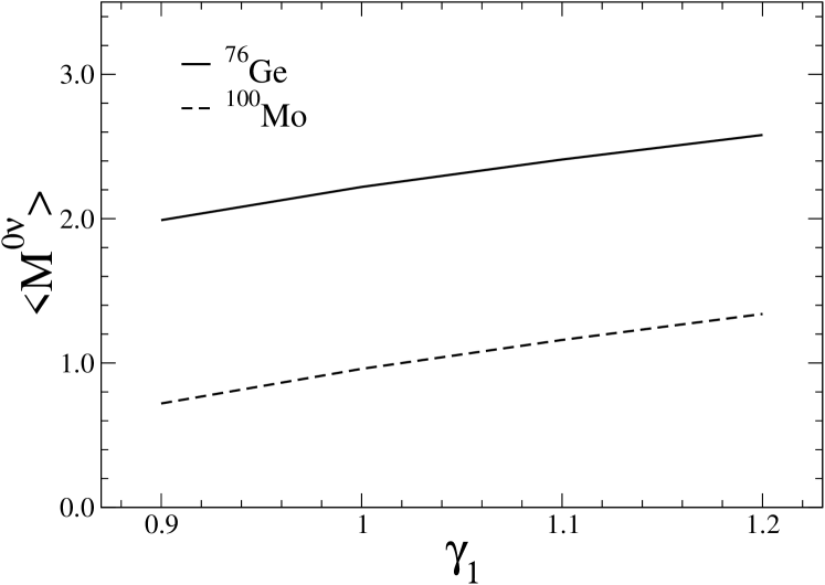
Figure 1: Nuclear matrix element ${M^{\prime}}^{0\nu}$ as function of parameter $\gamma_{1}$ of the function $f(r_{12})$, Eq. (11), used to account for the two-nucleon short range correlations. Calculation performed in RQRPA with $g_{pp}=0.99~{}(^{76}Ge),~{}1.21~{}(^{100}Mo)$ and the small single particle level scheme.

Another uncertainty is related to the treatment of the short range nucleon correlation. The adopted form of the Jastrow-type factor $f(r_{12})$, Eq. (11), is based on the work MS1976 where a range of the values of the parameter $\gamma_{1}$ is given. We vary that parameter $\gamma_{1}$ from 0.9 to 1.2 ($\gamma_{2}$ is fully determined by $\gamma_{1}$). The calculated dependence of ${M^{\prime}}^{0\nu}$ is shown in Fig. 1 for ⁷⁶Ge and ¹⁰⁰Mo. One can see that over this range of $\gamma_{1}$ values the calculated results differ by only about 10% from the ones corresponding to $\gamma_{1}=1.1$ used in the standard calculations.

Since $M^{2\nu}$ is not affected by the short range repulsion, Fig. 1 simply shows that the $0\nu\beta\beta$ matrix elements ${M^{\prime}}^{0\nu}$ are not very sensitive to reasonable variations of the parameter $\gamma_{1}$ foot2 .

Combining the average $\langle{M^{\prime}}^{0\nu}\rangle$ with the phase-space factors, the expected half-lives (for RQRPA and $\langle m_{\nu}\rangle$ = 50 meV, the scale of neutrino masses suggested by oscillation experiments) are also shown in Table 1 (column 7).

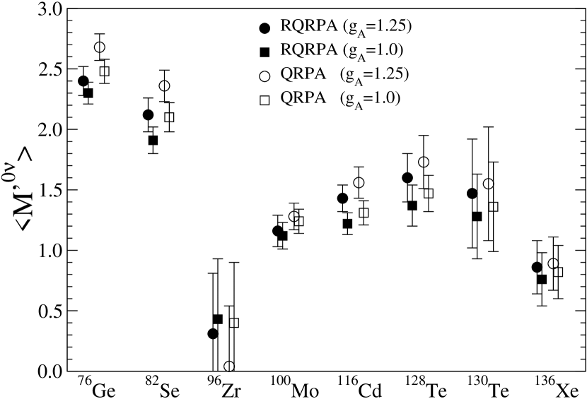
Figure 2: Average nuclear matrix elements $\langle{M^{\prime}}^{0\nu}\rangle$ and their variance (including the error coming from the experimental uncertainty in $M^{2\nu}$) for both methods and for all considered nuclei. For ¹³⁶Xe the error bars encompass the whole interval related to the unknown rate of the $2\nu\beta\beta$ decay.

The information collected in Table 1 is presented in graphical form in Fig. 2. There the averaged nuclear matrix elements for both methods and both choices of $g_{A}$ are shown along with their full uncertainties (theoretical plus experimental).

The entries for ¹³⁰Te are slightly different from the corresponding results in Ref.Rod03a . This is so because in the present work we use the $2\nu\beta\beta$ lifetime tentatively determined in the recent experiment Cuore , while in Rod03a we used the somewhat longer $2\nu\beta\beta$ lifetime based on the geochemical determination geoch .

II.2 Preliminary discussion of the procedure

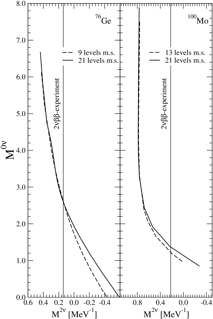
Figure 4: Dependence of the matrix elements ${M^{\prime}}^{0\nu}$ on $M^{2\nu}$ originating from the variation of the parameter $g_{pp}$ only. The results were obtained within the QRPA approach. The vertical lines show the experimental $M^{2\nu}$ values used for the $g_{pp}$ adjustment.

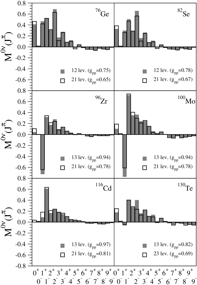
Figure 5: Multipole decomposition of the matrix elements ${M^{\prime}}^{0\nu}$ calculated within the QRPA. $J^{\pi}$ is the angular momentum and parity of the virtual intermediate state.

One can qualitatively understand why our chosen procedure stabilizes the ${M^{\prime}}^{0\nu}$ matrix elements as follows: The $M^{2\nu}$ matrix elements involve only the $1^{+}$ (virtual) states in the intermediate odd-odd nucleus. The nuclear interaction is such that the Gamow-Teller correlations (spin one, isospin zero pairs; after all the deuteron is bound and the di-neutron is not) are very near the corresponding phase-transition in the $1^{+}$ channel (corresponding to the collapse of the QRPA equations of motion). The contributions of the $1^{+}$ multipole for both modes of the $\beta\beta$ decay ($2\nu$ and $0\nu$) depends therefore very sensitively on the strength of the particle-particle force, parameterized by $g_{pp}$. On the other hand, the ${M^{\prime}}^{0\nu}$ matrix element, due to the presence of the neutrino propagator, depends on states of many multipolarities in the virtual intermediate odd-odd nucleus. The other multipoles, other than $1^{+}$, correspond to small amplitudes of the collective motion; there is no instability for realistic values of $g_{pp}\sim 1.0$. Hence, they are much less sensitive to the value of $g_{pp}$. In the four panels of Fig. 3 we show the $g_{pp}$ dependence of the contribution of the $1^{+}$ multipole on one hand and of all the other multipoles added on the other hand. Remembering that the nominal value of $g_{pp}$ is $\sim 1.0$, one can clearly see the large difference in the corresponding slopes. By making sure that the contribution of the $1^{+}$ multipole is fixed, we therefore stabilize the ${M^{\prime}}^{0\nu}$ value. The fact that RQRPA essentially removes the instability becomes then almost irrelevant thanks to the chosen adjustment of $g_{pp}$. The effect of stabilization against the variation of the basis size is seen clearly if one plots directly ${M^{\prime}}^{0\nu}$ versus $M^{2\nu}$, Fig. 4. Also the obtained multipole decompositions of ${M^{\prime}}^{0\nu}$ plotted in Fig. 5 show the essential stability of the partial contributions against variation of the basis size. (Note that in the case of ${}^{96}Zr$ our approach gives rather small matrix element and its uncertainty is even compatible with zero value. The smallness of that matrix element is due to a large negative contribution of the $1^{+}$ multipole, see Fig. 5).

Since the $2\nu$ lifetime depends on the square of $M^{2\nu}$, there is an ambiguity in choosing the sign of the $M^{2\nu}$, and hence the corresponding value of $g_{pp}$. In this work, and in Ref.Rod03a , always the solution corresponding to the smaller $g_{pp}$ value is chosen (positive $M^{2\nu}$ with the present phase convention). It is worthwhile to justify such a choice. There are several reasons why the smaller $g_{pp}$ should be used. First, QRPA and RQRPA are methods designed to describe small amplitude excitations around the mean field minimum. Were we to choose the larger value of $g_{pp}$, close or past the critical ‘collapse’ value, the method would be less likely to adequately describe the corresponding states. Second, as we will show later, by choosing the larger $g_{pp}$ the disagreement between the experimental and calculated rate of the single beta transitions from the lowest $1^{+}$ state in the intermediate nucleus would be far worse than with the smaller $g_{pp}$. Moreover, as shown in Ref. deform , only with the smaller $g_{pp}$ can one successfully describe the systematic of single beta decay in a variety of nuclei. It follows from the study of Ref. homma that choosing the larger value of $g_{pp}$ (i.e., the negative sign of $M^{2\nu}$) would lead to a complete disagreement with the systematics of single beta decays. Finally, there is also a pragmatic argument for such a choice. Only with it, the $0\nu$ nuclear matrix element becomes independent of the size of the single particle basis. Thus, this choice, admittedly ad hoc, removes the dependence on many more essentially arbitrary choices.

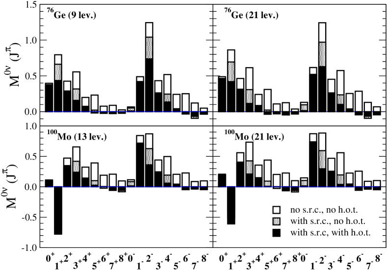
Figure 6: The effects of higher-order terms of nucleon currents (h.o.c.) and of the nucleon-nucleon short range repulsion (s.r.c.) on the multipole distribution of the $0\nu\beta\beta$-decay matrix element in the QRPA. The left panels were calculated with 9(13) single-particle levels and the right panels with 21 single-particle levels.

One can see in Fig.5 that all multipoles $J^{\pi}$ (see Eq.(10)), with the exception of the $1^{+}$ and various very small entries, contribute with the same sign. This suggests that uncertainties in one or few of them will have relatively minor effect. It is instructive to see separately the effect of the sometimes neglected short-range repulsive nucleon-nucleon repulsion and of the induced weak nucleon currents. These effects are shown in Fig. 6. One can see in that figure that the conclusion of the relative role of different multipoles is affected by these terms. For example, in ¹⁰⁰Mo the $1^{-}$ multipole is the strongest one when all effects are included, while the $2^{-}$ becomes dominant when they are neglected.

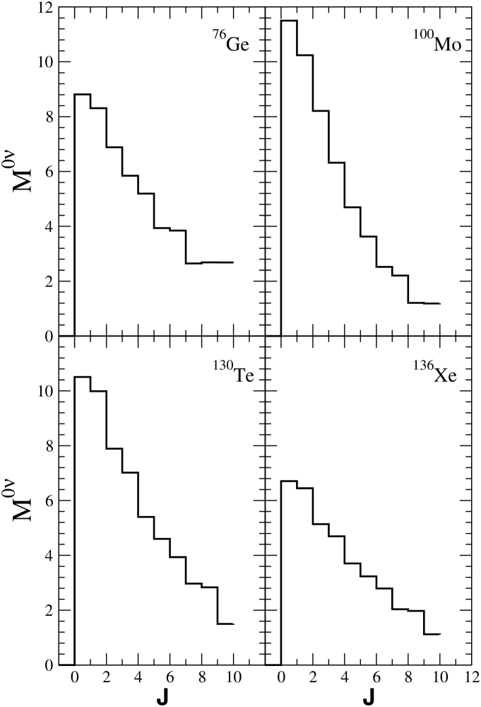
Figure 7: Running sum of the $0\nu\beta\beta$ decay matrix element as a function of the angular momentum ${\mathcal{J}}$ of the $nn$ and $pp$ pair that undergoes transition.

It is worthwhile to point out that one can display various contributions to ${M^{\prime}}^{0\nu}$ in an alternative, perhaps more revealing, way. Instead of $J^{\pi}$ that represents virtual states in the intermediate odd-odd nucleus, one can decompose the result in terms of ${\mathcal{J}}$, the angular momentum of the neutron-neutron (and simultaneously proton-proton) pair that undergoes the transition. In that case ${\mathcal{J}}=0^{+}$ represents the ‘pairing only’ contribution, while ${\mathcal{J}}\neq 0^{+}$ come from the ground state correlations, i.e., contributions from higher seniority (broken pairs) states. In Fig. 7 we show that these higher seniority states contributions consistently have the tendency to cancel the ‘pairing only’ piece. Thus, the final ${M^{\prime}}^{0\nu}$ is substantially less than the ${\mathcal{J}}=0^{+}$ part only, signifying the importance of describing the ground state contributions properly. (This tendency is a well known effect, for both modes of the $\beta\beta$ decay. It has been discussed, e.g. in Ref. gensen .)

III Uncertainties of the $0\nu\beta\beta$ decay matrix elements

One cannot expect that the QRPA-like and shell model calculations will lead to identical results due to substantial differences between both approaches. (However, we point out below that the results of the present approach and the shell model results differ relatively little whenever a comparison is possible.) Our goal in this section is to show that a majority of differences among various QRPA-like calculations can be understood. In addition, we discuss the progress in the field and possible convergence of the QRPA results. Based on our analysis, we suggest that it is not appropriate to treat all calculated $0\nu\beta\beta$-decay matrix elements at the same level, as it is commonly done (see e.g., bah04 ; CS03 ), and to estimate their uncertainty based on their spread.

Here we shall discuss the differences among different published QRPA and RQRPA results. We shall not consider the problem of the proton-neutron pairing in the double beta decay pan96 and the self-consistent RQRPA (SRQRPA) calculations bob01 . A systematic study of the $0\nu\beta\beta$-decay matrix elements within the SRQRPA will be discussed in a forthcoming publication, where we show that within the considered approach of fixing nuclear structure input Rod03a the results agree well with those obtained within the QRPA and the RQRPA.

Representative examples of the nuclear matrix elements calculated by different authors within the QRPA and RQRPA for nuclei of experimental interest are collected in Table 2. In order to understand the differences between the entries, let us enumerate the main reasons leading to a spread of the published QRPA and RQRPA results:

• i) The quasiparticle mean field. Since the model space considered is finite, the pairing interactions have been adjusted to fit empirical pairing gaps based on the nuclear binding energies. This procedure is followed practically by all authors. However, it fails for closed proton (¹¹⁶Sn) and neutron (¹³⁶Xe) shells. Some authors CS03 modify the single particle energies (mostly spherical Woods-Saxon energies) in the vicinity of the Fermi surfaces to reproduce the low-energy quasiparticle spectra of the neighboring odd-mass nuclei.

• ii) Many-body approximations. The RQRPA goes beyond the QRPA by partially taking into account Pauli principle violation in evaluation of the bifermion commutators. Based on that, one might expect that the RQRPA is more accurate than the unrenormalized QRPA. Calculations within solvable models sim01 support this conjecture.

• iii) Nucleon-nucleon interaction. In the $0\nu\beta\beta$-decay calculations both schematic zero-range Engel88 and realistic interactions were considered. In Ref. mut89 $G$-matrix of the Paris potential approximated by a sum of Yukawa terms was used. The interaction employed by the Tuebingen group has been the Brueckner $G$ matrix that is a solution of the Bethe-Goldstone equation with Bonn (Bonn CD, Argonne, Nijmegen) one boson exchange potential. The results do not depend significantly on the choice of the NN interaction Rod03a .

• iv) The renormalization of the particle-hole interaction. This is achieved by scaling the particle-hole part of the (R)QRPA matrix by the parameter $g_{ph}$. That parameter is typically adjusted by requiring that the energy of some chosen collective state, often the giant Gamow-Teller (GT) resonance, is correctly reproduced. In Ref. Rod03a it was found that the GT state is almost independent of the size of the model space and is well reproduced with $g_{ph}\approx 1$. In Refs. pan96 ; si99 $g_{ph}=0.8$ was chosen and in Ref. suh91 $g_{ph}=1.3$ was considered for $A>114$ nuclei. The sensitivity of results to the change of $g_{ph}$ were studied in Ref. bob01 where it was shown that for $0.8\leq g_{ph}\leq 1.0$ the change of the RQRPA $0\nu\beta\beta$-decay matrix element does not exceed 10%.

• v) The renormalization of the particle-particle interaction. This is achieved by scaling the particle-particle part of the (R)QRPA matrix by the parameter $g_{pp}$. When the early QRPA calculation were performed, only a limited information about the experimental $2\nu\beta\beta$-decay half-lives was available. Thus, in Ref. Engel88 a probable $g_{pp}$ window was estimated from $\beta^{+}$ decays of semi-magic nuclei. In another work mut89 systematics of the $pp$-force were investigated by an analysis of the single $\beta^{+}/EC$ decays. Alternatively, in many works $g_{pp}=1.0$ was chosen si99 ; pan96 ; bob01 ; suh91 ; tom91 . Nowadays, the $2\nu\beta\beta$-decay has been observed in ten nuclides, including decays into two excited states data . Two recent papers used the $2\nu\beta\beta$-decay half-lives to fix the strength of the particle-particle interaction of the nuclear Hamiltonian. In Ref. SK01 it was used only for the $J^{\pi}=1^{+}$ channel leaving the particle-particle strength unrenormalized (i.e., $g_{pp}=1.0$) in other channels. In our previous paper Rod03a , and in the current work, $g_{pp}$ is adjusted so that the $2\nu\beta\beta$-decay rate is correctly reproduced. The same $g_{pp}$ is used for all multipole channels of the particle-particle interaction. Since information that can be used to adjust the $g_{pp}$ value exists only for the $1^{+}$ channel, we cannot make a separate adjustment for other multipoles. Our economical choice is then to use the same $g_{pp}$ for all multipoles. That makes the hamiltonian as simple as possible, and preserves the relative strength of different multipoles of the realistic starting point interaction. On the other hand, some authors prefer to fix the $g_{pp}$ value to the $\beta^{-}$ decay transition of the ground state of the intermediate nucleus CS03 . Such procedure can be carried out, however only for three nuclear systems (A=100, 116 and 128) where $1^{+}$ is the ground state of the intermediate nucleus. Since forbidden decays are less well understood than the allowed ones it is difficult to rely on them in the case of other nuclear systems. (We discuss in more detail the differences between these two approaches of fixing the parameter $g_{pp}$ in the next section.)

• vi) The size of the model space. A small model space comprising usually of two major shells was often used in the calculation of the nuclear matrix elements CS03 ; SK01 ; Engel88 ; mut89 ; suh91 ; tom91 . Significantly larger model space has been used in Refs.Rod03a ; si99 consisting of five major shells. As a rule the results obtained for the large model space are reduced when compared to those for the small model space for the same value of $g_{pp}\sim 1$. The dependence of the calculated nuclear matrix elements on the size of the model space has been studied in Ref.SK01 and in Rod03a . Rather different conclusions using the same procedure of fixing $g_{pp}$ was reached. The origin of such discrepancy is not understood. In Ref. SK01 relatively small differences between model spaces were considered and a large effect on the $0\nu\beta\beta$-decay matrix element was found. In particular, by adding the $N=2$ shell to the $N=3-4$ oscillator shell model space the $0\nu\beta\beta$-decay matrix element of ${}^{76}Ge$ decreased by a factor of about 3 (see Table 2). Thus, in Ref. SK01 the single-particle levels lying far from the Fermi surface seem to influence strongly the decay rate. In contrast, in Ref. Rod03a and in the present work results essentially independent on the size of the basis have been found even with significantly different sizes of the model space.

• vii) The closure approximation. The $0\nu\beta\beta$-decay matrix elements were usually calculated using the closure approximation for intermediate nuclear states SK01 ; Engel88 ; mut89 ; tom91 . Within this approximation energies of intermediate states ($E_{n}-E_{i}$) are replaced by an average value ($<E_{n}-E_{i}>\approx 10~{}MeV$), and the sum over intermediate states is taken by closure, $\sum_{n}|J^{\pi}_{n}><J^{\pi}_{n}|=1$. This simplifies the numerical calculation drastically. The calculations with exact treatment of the energies of the intermediate nucleus were presented in Ref. Rod03a ; si99 ; pan96 . The effect of the closure approximation was studied in details in Ref. mut94 . It was found that the differences in nuclear matrix elements are within $10\%$. This is so because the virtual neutrino has an average momentum of $\sim 100$ MeV, considerably larger than the differences in nuclear excitation energies.

• viii) The axial-vector coupling constant $g_{A}$. The axial-vector coupling constant or in other words, the treatment of quenching, is also a source of differences in the calculated nuclear matrix elements. The commonly adopted values are $g_{A}=1.0$ Engel88 and $g_{A}=1.25$ Rod03a ; si99 ; pan96 ; mut89 ; tom91 . However, as shown in Table 2, if $g_{pp}$ is fixed to the $2\nu\beta\beta$-decay half-life, the effect of $g_{A}$ modification is smaller, of order $10\%$.

• ix) The two-nucleon short-range correlations (s.r.c.). In majority of calculations the short-range correlations between two nucleons are taken into account by multiplying the two-particle wave functions by the correlation function MS1976 : $f(r)=1-e^{-\gamma_{1}r^{2}}(1-\gamma_{2}r^{2})$ with $\gamma_{1}=1.1$ fm^-2 and $\gamma_{2}=0.68$ fm^-2. The sensitivity of results to the change of this parameters have been discussed in the previous section. It is also known that the $0\nu\beta\beta$-decay matrix element is more affected (reduced) by the s.r.c. at higher $g_{pp}$ values. We note that the s.r.c. were not taken into account within the approach which was developed in Ref.suh91 and used in the recent publication CS03 . For the realistic $g_{pp}$ values neglecting s.r.c. would lead to an increase in $M^{0\nu}$ by factor of about 2.

• x) The higher order terms of the nucleon current. The momentum dependent higher order terms of nucleon current, namely the induced pseudoscalar and weak magnetism, were first considered in connection with the light neutrino mass mechanism of the $0\nu\beta\beta$-decay in si99 . Their importance is due to the virtual character of the exchanged neutrino, with a large average momentum of $\sim$ 100 MeV. The corresponding transition operators have different radial dependence than the traditional ones. It is worth mentioning that with modification of the nucleon current one gets a new contribution to neutrino mass mechanism, namely the tensor contribution. The corrections due to the induced pseudoscalar nucleon current vary slightly from nucleus to nucleus, and in all cases represent about $30\%$ reduction. In the present calculation the effect of higher order terms of nucleon current is taken into account.

• xi) The finite size of the nucleon is taken into account via momentum dependence of the nucleon form-factors. Usually this effect on the $0\nu\beta\beta$-decay matrix elements associated with light neutrino exchange is neglected Engel88 ; tom91 , since it is expected to be small. In the presented calculation it is taken account by assuming phenomenological cutoff (see si99 and references therein). We found that by considering the finite nucleon size the value of ${M^{\prime}}^{0\nu}$ is reduced by about 10%. In Refs. suh91 ; CS03 the nucleon current is treated in a different way than in other double beta decay studies, namely it is evaluated from the quark level using relativistic quark wave functions. However, the momentum dependence of corresponding nucleon form-factors is not shown, so a comparison is difficult. Comparing the present results with those of Ref. suh91 for the same nuclear structure input suggests that the agreement might be achieved only if a very low cutoff is introduced.

• xii) The overlap factor of intermediate nuclear states. This factor is introduced since the two sets of intermediate nuclear states generated from initial and final ground states are not identical within the considered approximation scheme. A majority of calculations uses a simple overlap factor $X^{i}X^{f}-Y^{i}Y^{f}$, inspired by the orthogonality condition of RPA states generated from the same nucleus. However, the double beta decay is a two-vacua problem. The derivation of the overlap matrix within the quasiboson approximation scheme was performed in Refs.overl ; deform . It was shown that the overlap factor of the initial and final BCS vacua is an integral part of the overlap factor of the intermediate nuclear states deform ; grotz . This BCS overlap factor, about 0.8 for spherical nuclei, is commonly neglected in the calculation of nuclear matrix elements. If one fits $g_{pp}$ to the experimental $2\nu\beta\beta$-transition probability, the effect of the BCS overlap factor is significantly reduced. Hence it is neglected in the present work. This factor has been found to be important in the calculation within the deformed QRPA.

• xiii) The nuclear shape. Until now, in all QRPA-like calculations of the $0\nu\beta\beta$-decay matrix elements the spherical symmetry was assumed as the majority of nuclei of experimental interest are nearly spherical. The effect of deformation on the $0\nu\beta\beta$-decay matrix elements has not been studied as of now. Recently, the $2\nu\beta\beta$-decay matrix elements were calculated within the deformed QRPA with schematic forces deform . It was found that differences in deformation between initial and final nuclei have a large effect on the $2\nu\beta\beta$-decay half-life. One could expect that a similar mechanism of suppression of nuclear matrix elements is present also in the case of the $0\nu\beta\beta$-decay. It goes without saying that a further progress concerning this topics is highly desirable. The deformed QRPA might be the method of choice for the description of double beta decay of heavy nuclei like ¹⁵⁰Nd, or ¹⁶⁰Gd. However, the deformation of many medium heavy nuclear systems are also noticeable (see Table II of deform ). The main difficulty of the deformed RQRPA calculation is the fact that by going from the spherical to the deformed nuclear shapes the number of configurations increases drastically.

The present Table 2, is organized as follows: i) The results with and without inclusion of higher order terms of nucleon current are separated. We point out that in Refs. CS03 ; suh91 ; au98 the contribution from the weak-magnetism was taken into account. It is, however, negligible and we present their results without this contribution. ii) We indicate those matrix elements, which differ significantly from the present ones or other previous calculations (denoted as SK-01 SK01 and CS-03 CS03 ). We shall discuss this problem in detail below. iii) Within the sub-blocks the nuclear matrix elements are presented in ascending order following the year they appeared.

Many nuclear matrix elements in Table 2 were calculated from the published ratios of Fermi $M^{0\nu}_{F}$ and Gamow-Teller $M^{0\nu}_{GT}$ contributions and the absolute values of $|M^{0\nu}_{GT}|$ presented in units of fm^-1, i.e., not scaled with nuclear radius pan96 ; suh91 ; tom91 ; au98 We assumed that $R=r_{0}A^{1/3}$ with $r_{0}=1.1$ fm. However, Ref. mut89 used $r_{0}=1.2$ fm, so we rescaled the results in order to compare them better with ours. The differences between many calculations are understandable just from the way $g_{pp}$ was fixed, the considered size of the model space, the inclusion of the short-range correlation, the way the finite nucleon size is taken into account and other minor effects. Some nuclei, like ¹⁰⁰Mo, exhibit more sensitivity to these effects than others, such as ⁷⁶Ge or ⁸²Se. That is confirmed by our numerical studies.

The calculations of the $0\nu\beta\beta$-decay matrix elements by Civitarese and Suhonen CS03 (denoted as CS-03 in Table 2) deserves more comments. The authors performed them within the approach suggested in Ref. suh91 , (SKF-91) which employs the nucleon current derived from the quark wave functions. In this approach the two nucleon short-range-correlations are not taken into account. But, the contribution from higher order terms of nucleon current is studied. Unlike the present results the authors of Ref.suh91 claim that contribution from the induced pseudoscalar coupling is a minor one and they do not include it. At the same time, they find that the contribution from the weak-magnetism is negligible suh91 , in agreement with our result and with the $1/m_{p}^{2}$ scaling.

In Ref. suh91 the $g_{pp}$ was taken to be unity. The extension of this work for the case when $g_{pp}$ is adjusted to reproduce the single $\beta$-decay decay amplitudes was presented in Ref.au98 (AS-98) where also the effect of adjustment of the single particle energies to agree better with the spectroscopic data of odd-mass nuclei ($AS_{AWS}-98$) was studied. Since the adopted value of $g_{A}$ used for fixing $g_{pp}$ was not given, in Table 2 we present the corresponding ${M^{\prime}}^{0\nu}$ for both $g_{A}=1.0$ and $g_{A}=1.25$. (From the related article Suh04 it seems $g_{A}=1.0$ was considered.)

In Ref. CS03 (CS-03) the nuclear matrix elements are calculated in the same way as in au98 , however, the obtained results differ significantly (see Table 2) from each other. For some nuclei the difference is as large as a factor of two. There is no discussion of this there or in the later Refs. CS03 ; Suh04 . It is worth noticing that the largest matrix element in CS03 is found for the $0\nu\beta\beta$-decay of ¹³⁶Xe. This disagrees with the results of other authors (see Table 2). The reduction of the $0\nu\beta\beta$-decay of the ¹³⁶Xe is explained by the closed neutron shell for this nucleus. A sharper Fermi surface leads to a reduction of this transition.

Altogether, the matrix elements of Refs.au98 ; CS03 are noticeably larger than the present ones. Most of that difference can be attributed to the neglect of the short range nucleon-nucleon repulsion and of the higher order effects in the nucleon weak current in these papers.

As the above list of 13 points shows, there are many reasons, some more important than others, that might cause a difference between various calculated $0\nu\beta\beta$ matrix elements. Clearly, when some authors do not include effects that should be included (e.g. the short range correlations or the higher order terms in the nucleon current) their results should be either corrected or convincing arguments should be given why the chosen procedure was adopted. Other effects on the list are correlated, like the size of the model space and the renormalization of the particle-particle interaction. Again, if those correlations are not taken into account, erroneous conclusion might be drawn. Yet other effects are open to debate, like the quenching of $g_{A}$ or the adopted method of adjusting $g_{pp}$. In our previous work Rod03a , and in the present one, we show that our chosen way of renormalization removes, or at least greatly reduces, the dependence of the final result on most of the effects enumerated above.

Our choice of $g_{pp}$ adjustment, to the experimental $2\nu\beta\beta$ rate was used also in Refs.SK01 ; Muto97 . Let us comment on their results. Note, that the higher order corrections (h.o.c.) to the weak nucleon current were neglected in those works, hence one expects a $\sim$ 30% discrepancy right away.

In Ref. Muto97 only the $\beta\beta$ decay of ⁷⁶Ge was considered within both the QRPA and RQRPA. Only one s.p. basis was used, corresponding to the small one in our notation. The result was $M^{0\nu}=4.59\ (3.88)$ within QRPA (RQRPA). If one takes into account that h.o.c. as a rule reduce $M^{0\nu}$ by about 30% and the fact that $\sim$ 10% larger nuclear radius was used, one concludes that these matrix elements should be multiplied by $\sim$ 0.6 in order to compare them with our calculations. This results in $M^{0\nu}=2.76\ (2.34)$ which are in a very good agreement with our calculated $M^{0\nu}=2.68\ (2.41)$ for this case. Hence QRPA and RQRPA gave quite similar results in that case.

In contrast, the conclusions in Ref. SK01 are quite different from ours; the authors found significant dependence of their results on both the nuclear model and on the s.p. basis size, in spite of the adjustment of $g_{pp}$. The reason for these differences is unknown. In an attempt to understand the origin of them we comment here on features that, in our judgment, require further discussion.

1) We have already pointed out that the $M^{0\nu}$ for ⁷⁶Ge in Ref. SK01 changes with changing the single-particle basis within QRPA - from 4.45 (9 levels) to 1.71 (12 levels), or more than 2.5 times. This was obtained by adding just the deep-lying $sd$ shell, a surprising result.

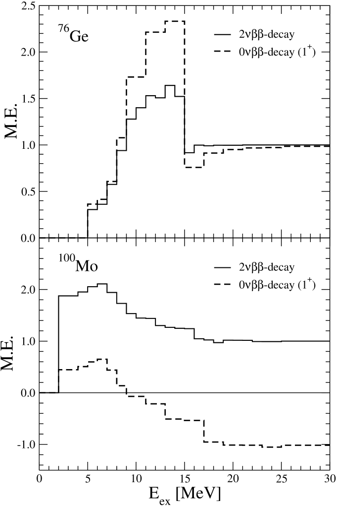
Figure 8: Running sum of the $2\nu\beta\beta$-decay and $0\nu\beta\beta$-decay (only $1^{+}$ component) matrix elements for ${}^{76}Ge$ and ${}^{100}Mo$ (normalized to unity) as a function of the excitation energy $E_{ex}=E_{n}-(E_{i}+E_{f})/2$. Calculations were performed within the QRPA.

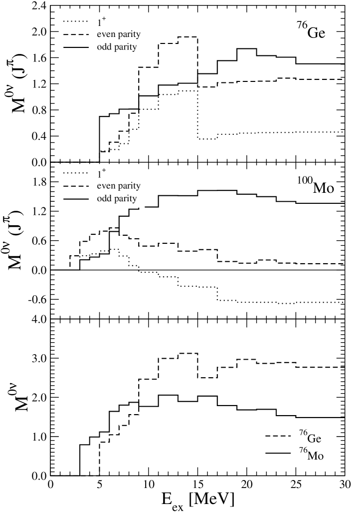
Figure 9: Running sum of the $0\nu\beta\beta$-decay matrix element for ${}^{76}Ge$ and ${}^{100}Mo$ and their multipole contributions as a function of excitation energy $E_{ex}=E_{n}-(E_{i}+E_{f})/2$. Calculations were performed within the QRPA (small model space).

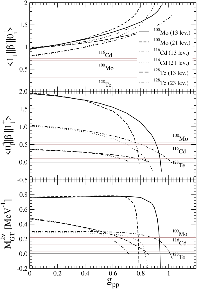
Figure 10: The upper panel: The matrix element associated with the $\beta^{-}$ transition from the initial nucleus (A,Z) to the $1^{+}$ ground state of the intermediate nucleus (A,Z+1) as function of $g_{pp}$ for ${}^{100}Mo$, ${}^{116}Cd$ and ${}^{128}Te$. The middle panel: The same as upper panel for the $\beta^{-}$ transition from the ground state of (A,Z+1) to ground state of final nucleus (A,Z+2). The lower panel: The $2\nu\beta\beta$-decay matrix element of ${}^{100}Mo$, ${}^{116}Cd$ and ${}^{128}Te$ as a function of $g_{pp}$. The experimental values are indicated by thin horizontal lines ($g_{A}=1.25$ is considered).

2) The last of the three papers contains most information and we can use their Figs. 1-14 with $M^{2\nu}$ and Figs. 15-25 with $M^{0\nu}$, in order to compare the numbers in the first (QRPA) and the last (SQRPA) columns of their Table 3. We were able to reproduce the entries in the QRPA column, but almost all entries in the SQRPA column, apart from those for ⁸²Se and ${}^{76}Ge$, seem inconsistent. The most striking difference is for ¹³⁶Xe. By inspecting Fig. 7 in SK01 , one finds that the appropriate $g_{pp}$ for SQRPA is about 1.08 (lines a and b). Now, by going to Fig. 24 one can see that the corresponding values of $M^{0\nu}$ are about 2.5 (lines c and d) while the entries in Table 3 are 0.98 and 1.03.

3) Some of the results in SK01 (see Fig.1, lines a and b, SQRPA; Fig.2, lines a and b, SQRPA, Fig.5, lines c and d, QRPA), Fig.7, lines c and d, QRPA) contradict the generally accepted conclusion that for all RPA-like approaches the functions $M^{2\nu}(g_{pp})$ calculated with the larger basis cross zero faster than the ones obtained with the smaller one. Thus, given these apparent inconsistencies, it is difficult to draw any conclusions from the comparison of our and Ref. SK01 results.

As pointed out above, one cannot expect a perfect agreement between the present result and the large scale shell model results SM96 . The approximations are different, and the shell model calculations do not include several multipoles (which typically enhance the matrix elements, see Fig. 5). Yet, remarkably, the present results and the published large scale shell model results agree with each other considerably better than the various entries in Table 2. So, using the published values, SM99 , we find ${M^{\prime}}^{0\nu}$ values 1.5, 2.1, 1.1, and 0.7 for ⁷⁶Ge, ⁸²Se, ¹³⁰Te and ¹³⁶Xe, while RQRPA gives 2.4, 2.1, 1.5, and 0.7-1.0 for the same nuclei. However, it appears that the more recent shell model results SM04 for ¹³⁰Te and ¹³⁶Xe give larger values while at the same time overestimating to some degree the rate of the $2\nu\beta\beta$ decay. In any case, we find this comparison encouraging.

IV Further discussion of the parameter adjustment

Ideally, the chosen nuclear structure method should describe all, or at least very many, experimental data and do that without adjustments. As described above that is not the case of QRPA or RQRPA. The interaction used is an effective interaction, and various parameters ($g_{pair},g_{ph},g_{pp}$) are adjusted. In particular, the parameters $g_{pair}$ and $g_{pp}$ are adjusted on the case-by-case basis in the present approach. Even then the method is not able to describe well all relevant weak transitions. In particular, it is sometimes impossible to describe simultaneously the $2\nu\beta\beta$ decay rate as well as the $\beta^{-}$ and $\beta^{+}/EC$ matrix elements connecting the $1^{+}$ ground states of the intermediate nucleus with the ground states of the final and initial nuclei (¹⁰⁰Mo is a well known example of this problem, see e.g. grif92 ).

Empirically, the transitions through the $1^{+}$ ground state of ¹⁰⁰Tc, ¹¹⁶In, and ¹²⁸I seemingly account for most of the $2\nu\beta\beta$ matrix element (this is the so called ‘Single State Dominance’ ssd ). Thus it appears that these single $\beta$ transitions are particularly relevant. Based on such considerations, Suhonen Suh04 suggested that the $\beta^{-}$ matrix element is more suitable source for the $g_{pp}$ adjustment than the $2\nu\beta\beta$ decay. Below we explain why we prefer the chosen method of parameter adjustment. On the other hand, we also argue that the adjustment based on the $\beta^{-}$ transitions might give results not far from ours, provided the independence on other adjustments can be proved.

First, it is not really true that the first $1^{+}$ state is the only one responsible for the $2\nu\beta\beta$ decay. This is illustrated for the cases of ⁷⁶Ge and ¹⁰⁰Mo in Fig. 8. Even though for ¹⁰⁰Mo the first state contributes substantially, higher lying states give non-negligible contribution. And in ⁷⁶Ge many $1^{+}$ states give comparable contribution. Thus, to give preference to the lowest state is not well justified, the sum is actually what matters. At the same time, the dilemma that the $\beta^{-}$ and $\beta^{+}/EC$ matrix elements move with $g_{pp}$ in opposite directions makes it difficult to choose one of them. It seems better to use the sum of the products of the amplitudes, i.e. the $2\nu\beta\beta$ decay.

At the same time, the contribution of the $1^{+}$ multipole to the $0\nu\beta\beta$ matrix element and the corresponding $2\nu\beta\beta$ matrix element are correlated, even though they are not identical, as shown in Fig. 8. Making sure that the $2\nu\beta\beta$ matrix element agrees with its experimental value constrains the $1^{+}$ part of the $0\nu\beta\beta$ matrix element as well.

In Fig. 9 we show the running sum contributions to the $0\nu\beta\beta$ matrix elements in ⁷⁶Ge and ¹⁰⁰Mo, separated into multipoles, and for the total. Such a sum, even for the $1^{+}$ component, is rather different that the similar staircase for the $2\nu\beta\beta$; there is no single state dominance. Thus, again, it is not obvious that it is best to choose any one particular state or transition for the adjustment. Moreover, while we have demonstrated that adjusting $g_{pp}$ to the $2\nu\beta\beta$ rate removes the dependence on other parameters, a similar proof was not given in Suh04 . Finally, as seen in Fig. 3 the slope of the $1^{+}$ multipole component of the $0\nu\beta\beta$ matrix element far exceeds the slope of the other multipoles. Hence, making sure that the whole $1^{+}$ multipole contribution is correct is crucial.

Thus, we prefer the method of adjustment used in the present work. That is so not only for the reasons shown above, but also because it is much more general as stressed already, while the ground state of the odd-odd nucleus has $1^{+}$ only in ¹⁰⁰Tc, ¹¹⁶In, and ¹²⁸I.

However, as demonstrated in the last figure, Fig. 10, the adjustment proposed in Ref. Suh04 , namely to choose the parameter $g_{pp}$ based on the $\beta^{-}$ decay of the intermediate $1^{+}$ state, would not be drastically different compared with the procedure used in the present work. As one could see, the resulting $g_{pp}$ are similar (but not identical) and the dependence on the s.p. basis will be also reduced (That important feature was not demonstrated in Ref. Suh04 , unfortunately). However, as the upper panel shows, it is difficult to describe the other component of that decay, the $\beta^{+}/EC$ amplitude. That is an obvious drawback of the QRPA method; it is never meant to describe in detail properties of non-collective states. But that is less relevant for the description of integral quantities that depend on sums over many states.

As pointed out earlier, we always choose the $g_{pp}$ corresponding to the positive $M^{2\nu}$ value. In the upper panel of Fig. 10 one can clearly see that were we to choose the other possibility, i.e., the $g_{pp}$ corresponding to the negative $M^{2\nu}$, the disagreement with the single beta decay would be considerably worse. It is important also to notice that if Pauli principle violation is restored (e.g. within the RQRPA) one finds that the solution corresponding to the negative value of $M^{2\nu}$ is out of physical interval of $g_{pp}$. This has been confirmed also in a schematic model by presenting the solution of the QRPA with full inclusion of the Pauli exclusion principle sim01 . As pointed out above, it was also found recently deform that for negative value of $M^{2\nu}$ the correspondence with particle-particle strength from systematic studies of the single beta decay homma is not achieved.

In this section we have summarized the arguments why we believe that the procedure of adjustment used in the present work is preferable to the procedure advocated in Ref.Suh04 . At the same time, we suggest that there is no fundamental difference between the two; both are used to fix the fast varying contribution of the $1^{+}$ multipole. The bulk of the matrix element is associated with the other multipoles, and their effect is much less dependent on relatively small variations of the parameter $g_{pp}$.

As we stressed already above, a substantial part of the differences in the calculated values of the $0\nu\beta\beta$ decay matrix elements has its origin not in the choice of $g_{pp}$ or other parameters, but in the neglect of the short range nucleon-nucleon repulsion and of the induced weak currents in some papers, and their inclusion in other papers (like the present one). Until a consensus on the treatment of these physics issues is reached, the differences in the calculated matrix elements cannot be avoided.

V Summary and conclusions

We have shown that the procedure suggested in our previous work, Ref. Rod03a , is applicable to essentially all nuclei with known $2\nu\beta\beta$ decay lifetimes . Adjusting the strength of the particle-particle neutron-proton force $g_{pp}$ in such a way that the experimental $2\nu\beta\beta$ decay rate is correctly reproduced removes much of the dependence on the size of the single-particle basis and whether QRPA or RQRPA is used. Here we also show that the quenching of the axial current matrix elements, parameterized by the reduction of the coupling constant $g_{A}$, also leaves the resulting $0\nu\beta\beta$ matrix elements almost unchanged; they become insensitive to the variations of parameters describing the short-range nucleon-nucleon correlations as well. Thus, the resulting $0\nu\beta\beta$ matrix elements acquire well defined values, free of essentially arbitrary choices. We also present arguments while we believe that the chosen procedure of adjusting the interaction is preferable to other proposed ways of adjustment.

We then summarize many published QRPA and RQRPA results and discuss their similarities and differences. We show that in most, albeit not all, cases these differences can be understood. We present an exhaustive list of reasons why individual calculated $0\nu\beta\beta$ nuclear matrix elements, evaluated within QRPA or RQRPA, might differ from each other. That list then can serve as a guide to readers of the past and future papers devoted to the subject. Comparison between the results of different QRPA/RQRPA calculations would be facilitated if authors of future publications specify in detail what choices of explicit and implicit adjustable parameters they made, and discuss the dependence of their result on their particular choice. We believe that by following these suggestions a consensus among the practitioners of QRPA/RQRPA could be reached and most of the spread between the calculated nuclear matrix elements, that causes much confusion in the wider physics community, would be shown to be essentially irrelevant. To reach a convergence of the results obtained using QRPA/RQRPA is clearly just an important step on the way to reliable and correct $0\nu\beta\beta$ decay nuclear matrix elements. Exploring the structure of the intermediate odd-odd nuclei by the charge exchange reactions would create an opportunity to test the nuclear models more thoroughly. Further progress in nuclear shell model calculations and in the exploration of the exactly solvable models could also point the way towards the ultimate solution of this important problem.

Table 1: Averaged $0\nu\beta\beta$ nuclear matrix elements $\langle{M^{\prime}}^{0\nu}\rangle$ and their variance $\sigma$ (in parentheses) evaluated in the RQRPA and QRPA. In column 6 the variance $\varepsilon_{exp.}$ of the $0\nu\beta\beta$-decay matrix element due to uncertainties in the measured $2\nu\beta\beta$-decay half-live $T^{2\nu-exp}_{1/2}$ is given. $M_{GT}^{exp}$ and $g_{A}$ denote the $2\nu\beta\beta$-decay nuclear matrix element deduced from $T^{2\nu-exp}_{1/2}$ and axial-vector coupling constant, respectively. In column 7 the $0\nu\beta\beta$ half-lives evaluated with the RQRPA average nuclear matrix element and for assumed $\langle m_{\beta\beta}\rangle$ = 50 meV are shown. For ¹³⁶Xe there are four entries; the upper two use the upper limit of the $2\nu$ matrix element while the lower two use the ultimate limit, vanishing $2\nu$ matrix element. ¹⁵⁰Nd is included for illustration. It is treated as a spherical nucleus; deformation will undoubtedly modify its $0\nu$ matrix element.

Nuclear	$~{}g_{A}~{}~{}$	$M_{GT}^{exp}$	$\langle{M^{\prime}}^{0\nu}\rangle$		$~{}~{}\varepsilon_{exp.}~{}~{}$	$T^{0\nu}_{1/2}$ ($\langle m_{\beta\beta}\rangle$ = 50 meV)
transition		$[MeV^{-1}]$	RQRPA	QRPA		[yrs]
${}^{76}Ge\rightarrow{{}^{76}Se}$	1.25	$0.15\pm 0.006$	2.40(0.07)	2.68(0.06)	$\pm 0.05$	$2.29_{-0.16}^{+0.17}~{}10^{27}$
	1.00	$0.23\pm 0.01$	2.30 (0.04)	2.48 (0.05)	$\pm 0.05$	$2.49_{-0.13}^{+0.15}~{}10^{27}$
${}^{82}Se\rightarrow{{}^{82}Kr}$	1.25	$0.10\pm 0.009$	2.12 (0.10)	2.36 (0.09)	$\pm 0.04$	$6.60_{-0.62}^{+0.73}~{}10^{26}$
	1.00	$0.16\pm 0.008$	1.91 (0.05)	2.10 (0.07)	$\pm 0.05$	$8.13_{-0.57}^{+0.64}~{}10^{26}$
${}^{96}Zr\rightarrow{{}^{96}Mo}$	1.25	$0.11^{+0.03}_{-0.06}$	0.31 (0.08)	0.04 (0.10)	${}^{+0.20}_{-0.43}$	$1.45_{-0.96}^{\infty}~{}10^{28}$
	1.00	$0.17^{+0.05}_{0.06}$	0.43 (0.11)	0.40 (0.02)	${}^{+0.25}_{-0.45}$	$0.77_{-0.48}^{\infty}~{}10^{28}$
${}^{100}Mo\rightarrow{{}^{100}Ru}$	1.25	$0.22\pm 0.01$	1.16(0.11)	1.28(0.09)	$\pm 0.02$	$1.36_{-0.23}^{+0.30}~{}10^{27}$
	1.00	$0.34\pm 0.015$	1.12 (0.09)	1.24 (0.08)	$\pm 0.02$	$1.45_{-0.21}^{+0.27}~{}10^{27}$
${}^{116}Cd\rightarrow{{}^{116}Sn}$	1.25	$0.12\pm 0.006$	1.43 (0.08)	1.56 (0.10)	$\pm 0.03$	$8.20_{-0.90}^{+1.07}~{}10^{26}$
	1.00	$0.19\pm 0.009$	1.22 (0.07)	1.31 (0.08)	$\pm 0.02$	$11.3_{-1.23}^{+1.48}~{}10^{26}$
${}^{128}Te\rightarrow{{}^{128}Xe}$	1.25	$0.034\pm 0.012$	1.60 (0.11)	1.73 (0.13)	$\pm 0.09$	$1.85_{-0.29}^{+0.38}~{}10^{28}$
	1.00	$0.053\pm 0.02$	1.37 (0.07)	1.47 (0.05)	$\pm 0.1$	$2.52_{-0.40}^{+0.52}~{}10^{28}$
${}^{130}Te\rightarrow{{}^{130}Xe}$	1.25	$0.036^{+0.03}_{-0.009}$	1.47 (0.15)	1.55(0.17)	${}^{+0.3}_{-0.09}$	$0.87_{-0.16}^{+0.25}~{}10^{27}$
	1.00	$0.056^{+0.05}_{-0.15}$	1.28 (0.08)	1.36 (0.10)	${}^{+0.27}_{-0.08}$	$1.15_{-0.38}^{+0.23}~{}10^{27}$
${}^{136}Xe\rightarrow{{}^{136}Ba}$	1.25	$0.030$	0.98(0.09)	1.03(0.08)		$1.84_{-0.30}^{+0.39}~{}10^{27}$
	1.00	$0.045$	0.90 (0.07)	0.94 (0.05)		$2.18_{-0.16}^{+0.25}~{}10^{27}$
	1.25	0	0.73(0.09)	0.77(0.10)		$3.32_{-0.69}^{+1.00}~{}10^{27}$
	1.00	0	0.63 (0.07)	0.67 (0.08)		$4.45_{-0.85}^{+1.18}~{}10^{27}$
${}^{150}Nd\rightarrow{{}^{150}Sm}$	1.25	$0.07^{+0.009}_{-0.03}$	2.05 (0.13)	2.25 (0.16)	${}^{+0.07}_{-0.20}$	$0.92_{-0.12}^{+0.26}~{}10^{26}$
	1.00	$0.11^{+0.014}_{-0.05}$	1.79 (0.05)	1.96 (0.04)	${}^{+0.06}_{-0.19}$	$1.21_{-0.10}^{+0.32}~{}10^{26}$

Table 2: Neutrinoless double beta decay matrix element ${M^{\prime}}^{0\nu}$ calculated within QRPA and RQRPA approaches. The way of fixing the particle-particle interaction strength is indicated: a given value, to $2\nu\beta\beta$-decay half-life, to $\beta$ decays. The nuclear radius is $R=r_{0}A^{1/3}$. Notation: EVZ-88 = Engel, Vogel, ZirnbauerEngel88 (for $\alpha_{1}^{\prime}$ = -390), MBK-89 = Muto, Bender, Klapdormut89 , T-91 = Tomoda tom91 , SKF-91 = Suhonen, Khadkikhar, Faesslersuh91 , PSVF-96 = Pantis, Šimkovic, Vergados, Faesslerpan96 , AS-98 = Aunola, Suhonenau98 , results for Woods-Saxon (WS) and adjusted Woods-Saxon (AWS) bases, SPVF-99 = Šimkovic, Pantis, Vergados, Faesslersi99 , SK-01 = Stoica, Klapdor-KleingrothausSK01 (the second line by SK-01 results corresponds to slightly larger model space), CS-03 = Civitarese, SuhonenCS03 .

Ref.	Method	$r_{0}$	$g_{pp}$	$g_{A}$	${M^{\prime}}^{0\nu}$
		[fm]			${}^{76}Ge$	${}^{82}Se$	${}^{96}Zr$	${}^{100}Mo$	${}^{116}Cd$	${}^{128}Te$	${}^{130}Te$	${}^{136}Xe$	${}^{150}Nd$
					Without higher order terms of nucleon current
					Differences understandable
EVZ-88	QRPA	1.1	$\beta$	1.0	1.3	1.0	0.8	1.8		2.4	2.2	1.0
MBK-89	QRPA	1.1	$\beta$	1.25	3.84	3.59		1.94		3.93	3.18	1.45	5.57
T-91	QRPA	1.1	1.0	1.0	2.86	2.59		3.14		2.55	2.22	1.27	3.47
				1.25	3.97	3.60		4.30		3.53	3.07	1.74	4.80
SKF-91	QRPA	1.1	1.0	1.00	3.37	2.72				3.17	2.94	1.71
				1.25	4.55	3.71				4.24	3.95	2.31
PSVF-96	QRPA	1.1	1.0	1.25	3.04	2.23	2.41	1.09	0.94	2.48	2.33	1.55
SPVF-99	RQRPA	1.1	1.0	1.00	4.05	3.82	2.24	4.58	2.86	3.38	2.87	1.20	5.15
				1.25	3.60	3.40	1.99	4.12	2.58	2.96	2.50	1.02	4.51
present	QRPA	1.1	$2\nu\beta\beta$	1.25	3.35	2.95		1.83		2.32	1.98	1.30	3.10
					Results discussed
SK-01	QRPA	?	$2\nu\beta\beta$	?	4.45	5.60	4.16	5.37	3.99	4.84	4.73	1.69
					1.71	4.71	2.75	3.81	2.85	3.43	3.77	1.35
	RQRPA	?	$2\nu\beta\beta$	?	3.74	4.30	3.01	4.36	3.61	4.29	4.55	1.57
					1.87	2.70	2.72	3.40	3.39	2.83	3.00	1.02
$AS_{WS}$-98	QRPA	1.1	$\beta$	1.00	3.98	3.69	2.88		2.21		4.62	2.49
				1.25	5.30	4.93	3.85		2.93		6.15	3.34
$AS_{AWS}$-98	QRPA	1.1	$\beta$	1.00	4.85	3.61	3.70		3.97		3.81	2.15
				1.25	6.44	4.82	3.96		5.25		5.05	2.84
CS-03	QRPA	?	$\beta$	1.25	3.33	3.44	3.55	2.97	3.75		3.49	4.64
					With higher order terms of nucleon current
SPVF-99	RQRPA	1.1	1.0	1.25	2.80	2.64	1.49	3.21	2.05	2.17	1.80	0.66	3.33
present	QRPA	1.1	$2\nu\beta\beta$	1.00	2.48	2.10	0.40	1.24	1.31	1.47	1.36	0.94	1.96
				1.25	2.68	2.36	0.04	1.28	1.56	1.73	1.55	1.03	2.25
	RQRPA	1.1	$2\nu\beta\beta$	1.00	2.30	1.91	0.43	1.12	1.22	1.37	1.28	0.90	1.79
				1.25	2.40	2.12	0.31	1.16	1.43	1.60	1.47	0.98	2.05

Figure 3: Contribution of the $1^{+}$ and all the other (summed) multipoles to the matrix elements ${M^{\prime}}^{0\nu}$ as a function of the parameter $g_{pp}$. The results were obtained within the RQRPA approach for the large model space. The dots indicate the $g_{pp}$ values that reproduce the known $2\nu$ decay rate.