Spherical Hartree-Fock calculations with linear momentum projection before the variation.

Abstract

Spherical Hartree–Fock calculations with projection onto zero total linear momentum before the variation are performed for the nuclei ⁴He, ¹²C, ¹⁶O, ²⁸Si, ³²S and ⁴⁰Ca using a density–independent effective nucleon–nucleon interaction. The results are compared to those of usual spherical Hartree–Fock calculations subtracting the kinetic energy of the center of mass motion either before or after the variation and to the results obtained analytically with oscillator occupations. Total energies, hole–energies, elastic charge form factors and charge densities and the mathematical Coulomb sum rules are discussed.

1 Introduction

We consider the nucleus as a closed system of interacting, non–relativistic nucleons. The homogenity of space requires that the total linear momentum of this system is conserved. Consequently the hamiltonian describing any particular nucleus cannot depend on the center of mass (COM) coordinate of its constituents, but (besides on spin– and isospin–quantum numbers) only on relative coordinates and momenta. The dependence on the total momentum is trivial : it describes the free motion of the total system and can always be transformed away by considering the system in its COM rest frame. We have then to solve the corresponding Schrödinger equation for the remaining “internal” hamiltonian. In principle this can be achieved by writing this hamiltonian in Jacobi coordinates. However, nucleons are fermions and thus do obey the Pauli principle. Since the Jacobi coordinates depend on all the nucleon coordinates, thus an explicit antisymmetrization of the wave functions is required as it is performed, e.g., in few–body physics. Being already there sometimes rather involved though still feasible, such an explicit antisymmetrization becomes impossible in the many–body system (e.g., the antisymmetrization of 20 like nucleons would require 20 factorial different terms). Thus in the many–body system the antisymmetrization usually is performed implicitely by expanding the wave functions in terms of Slater (or generalized Slater) determinants. In this way the Pauli principle is automatically fulfilled. The Slater determinants, however, depend on 3A instead of the allowed 3A-3 coordinates and thus contain contaminations due to the motion of the system as a whole, so called “spurious” admixtures. Galilei–invariance is broken.

This defect of almost all microscopic nuclear structure models has been recognised ref1. almost immediately after the development of the shell–model. It was shown later on ref2. that in case of pure harmonic oscillator configurations one can get rid of this problem by diagonalizing the (oscillator) COM hamiltonian and projecting all states not corresponding to the ground state of this operator out of the spectrum of the many nucleon hamiltonian. This procedure, however, requires the use of so called complete $n\hbar\omega$–spaces (since only then COM and internal excitations decouple exactly) and thus is of little help in most of the usual approaches to the nuclear many–body problem. A more general solution is the projection of the wave functions into the COM rest frame ref3. , which ensures translational– and, if performed before solving the corresponding Schrödinger equation (usually by variational methods) even full Galilei–invariance ref4. . The key idea of this projection is to superpose the wave function shifted all over normal space with identical weights and thus to achieve vanishing total linear momentum. Since the bound states of a nucleus are localized, this procedure always does converge (for scattering states a slightly different procedure has to be used ref13. ). The projection method has the advantage that it works in general model spaces as well as for general (non–oscillator) wave functions.

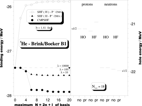
Figure 1: In the left part the total binding energy of ⁴He as obtained with the Brink–Boeker force B1 [14] using an oscillator length b=1.41 Fm is plotted against the size of the basis. Three curves are shown : the open circles correspond to a normal spherical Hartree–Fock calculation with the expectation value of $P^{2}/2MA$ subtracted after convergence, the full triangles display the results if this center of mass correction is included during the iteration, and, finally, the full circles give the result of a spherical Hartree–Fock calculation with projection into the momentum rest frame before the variation (CMPSHF). Furthermore, the figure displays the results of constrained calculations adding the oscillator center of mass Hamitonian with a Lagrangian multiplier $\lambda$ to the internal hamiltonian which “penalizes” COM excitations. The right part of the figure displays the hole energies obtained in the oscillator limit HO (N_max=0) and in the Hartree–Fock approximation HF (with N_max=18) using the “normal” (no) as well as the “projected” (pr) approach in both cases. Note that the normal approach includes the usual COM correction (see text).

Though in principle known since almost half a century, only few practical calculations have been performed using this method. The reason for this is quite simple : the projection operator is an A–body integral operator with the rather nasty property to link the usual model space states to rather highly excited (and thus usually unoccupied) ones as well as to the fully occupied ones, which are often treated as an inert core. This is easy to understand : any change of the linear momentum of the valence nucleons requires a corresponding change of the linear momentum of the core in order to ensure vanishing total linear momentum for the system. Unlike angular momentum, linear momentum is thus a true A–body correlation and hence much more complicated to treat than the latter.

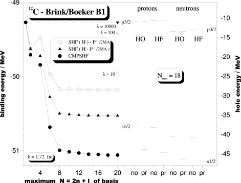
Figure 2: Same as in Fig. 1, but for the nucleus ¹²C with oscillator length b=1.72 Fm.

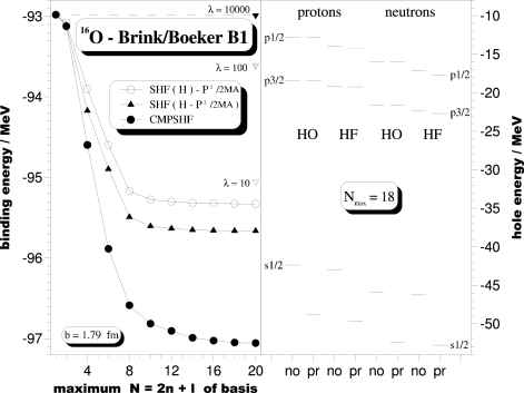
Figure 3: Same as in Fig. 1, but for the nucleus ¹⁶O with oscillator length b=1.79 Fm.

Because of these difficulties, instead of treating Galilei–invariance correctly, its breaking is usually neglected adopting the well known text book argument that it induces only 1/A effects and thus “can savely be neglected for nuclei beyond oxygen” ref4. , provided the usual approximate corrections like subtracting the kinetic energy of the COM motion from the original hamiltonian or the use of the so called Tassie–Barker factor ref5. in the analysis of form factors are done.

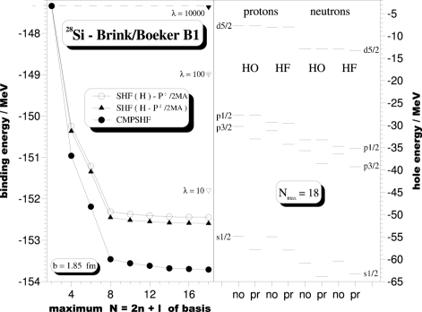
Figure 4: Same as in Fig. 1, but for the nucleus ²⁸Si with oscillator length b=1.85 Fm.

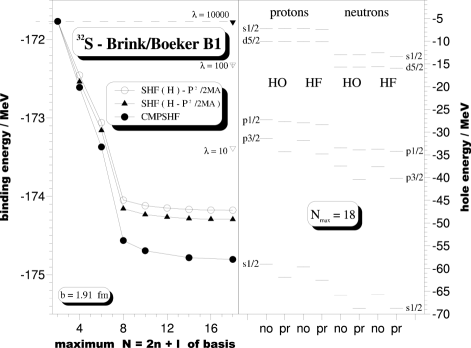
Figure 5: Same as in Fig. 1, but for the nucleus ³²S with oscillator length b=1.91 Fm.

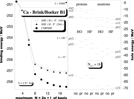
Figure 6: Same as in Fig. 1, but for the nucleus ⁴⁰Ca with oscillator length b=1.97 Fm.

That this, however, is not true has been shown by several studies within the last decade. Hartree–Fock calculations with projection into the COM rest frame for ⁴He [6] as well as the analysis of form factors and charge densities of several spherical nuclei ref7. ; ref8. have demonstrated that the correct treatment of Galilei–invariance yields considerable effects far beyond the usually assumed 1/A level. The same holds for scattering states as demonstrated in ref. ref9. for the inclusive quasi–elastic electron scattering again from ⁴He. Recently now, a whole series of model investigations ref10. ; ref11. ; ref12. ; ref13. has been published, in which the COM effects have been studied in a more systematic way. Considerable effects have been seen for spectral functions and spectroscopic factors, transition form factors and densities, energies of hole–states, Coulomb sum rules, response functions and many more. These investigations, however, have been undertaken with rather simple wave functions : the ground states of the doubly even A–nucleon systems ⁴He, ¹⁶O and ⁴⁰Ca have been described in the simple oscillator limit and for the ground and excited states of the corresponding odd (A-1)–nucleon systems simple one–hole states have been used. This has the advantage that all calculations can be performed analytically but is definitely not very realistic. So, e.g., the above mentioned pure oscillator A–nucleon configurations are non–spurious and thus the projection yields here no additional effect with respect to the usual approach to subtract the kinetic energy of the COM motion. It is hence desirable to study, e.g., these ground states in more realistic approaches. This will be done in this and a forthcoming paper.

For this purpose we have performed spherical Hartree–Fock calculations with projection into the COM rest frame before the variation for the six nuclei ⁴He, ¹²C, ¹⁶O, ²⁸Si, ³²S and ⁴⁰Ca. The results have been compared with those of normal spherical Hartree–Fock calculations subtracting the kinetic energy of the COM motion either before or after the variation and with the analytically obtained oscillator results out of ref. ref12. . For each of the considered nuclei up to 19 major oscillator shells have been used as single particle basis. As effective interaction the simple Brink–Boeker force B1 ref14. has been taken. We are aware of the fact that this interaction is not very realistic. However, the aim of the present investigation is not a comparison with experiment but the study of the effects of a correct treatment of Galilei–invariance. For this purpose the B1–interaction is as good as any other. Furthermore, consisting out of Gaussians, it can be treated in the oscillator limit analytically and thus allows for a direct comparison with the results reported in ref. ref12. .

Section 2 of the present paper gives a short summary of the spherical Hartree–Fock approach with projection into the COM rest frame before the variation. Section 3 will then describe some details of the calculations and present the results for the total energies, the hole–energies, the elastic charge form factors and corresponding charge densities and the Coulomb sum rules. Conclusions, three appendices with some detailed formulas and references conclude the present paper.

In the second of the present series of two papers we shall then discuss the effects of the correct treatment of Galilei–invariance on the spectral functions and spectroscopic factors obtained with the wave functions out of the present paper.

2 COM-projected Hartree-Fock.

The essential mathematics for Hartree–Fock calculations with projection into the COM rest frame before the variation has been presented in detail already in ref. [6] and hence will be summerized only briefly in the following. We start by defining our model space by $M_{b}$ oscillator single particle states, the creators of which will be denoted by $\{c^{{\dagger}}_{i}\,;\;i=1,...,M_{b}\}$. We shall furthermore assume that the effective hamiltonian appropriate for this model space is known and can be written in the chosen representation as a sum of only one– and two–body parts

$$\hat{H}\;=\;\sum_{ir}t(ir)c^{{\dagger}}_{i}c_{r}\;+\;\sum_{ikrs}v(ikrs)c^{{\dagger}}_{i}c^{{\dagger}}_{k}c_{s}c_{r}$$ (1)

where $t(ir)$ are the single particle matrix elements of the kinetic energy operator and $v(ikrs)$ the antisymmetrized two–body matrix elements of the considered interaction. We shall assume that this interaction is translational invariant, i.e., it does not depend on the center of mass coordinate of the two nucleons. Density dependent interactions (in their usual form) do not fulfill this requirement. Their treatment is much more complicated as has been described in detail in ref. ref12. . Such interactions will not be considered in the present paper.

In the Hartree–Fock approach one searches for the optimal one–determinant representation of the A–nucleon ground state having the form

$$|D\rangle\;=\;\left\{\prod_{h=1}^{A}\;b^{{\dagger}}_{h}\;\right\}|0\rangle\noindent$$ (2)

where

$$b^{{\dagger}}_{\beta}\;=\;\sum_{i=1}^{M_{b}}\;D^{*}_{i\beta}c^{{\dagger}}_{i}$$ (3)

and

$$b_{\beta}\;=\;\sum_{i=1}^{M_{b}}\;D_{i\beta}c_{i}$$ (4)

respectively, with $D$ being a unitary $(M_{b}\times M_{b})$ transformation. In eq. (2) we have assumed that the selfconsistent states created by the operators (3) are ordered according to their energy so that $\beta=1,...,A$ correspond to the occupied “hole” states $h,\;h^{\prime},\;...$. The unoccupied orbits $\beta=A+1,...,M_{b}$ will be denoted as “particle” states $p,\;p^{\prime},\;...$ in the following.

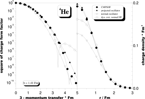
Figure 7: In the left part of the figure the square of the charge form factor for ⁴He is displayed as function of the 3–momentum transfer. For the nucleon form factors the usual dipole parametrisation [21] has been used. Open inverted triangles correspond to an oscillator occupation with no COM correction included (normal oscillator), full triangles give the oscillator result including the Tassie–Barker factor [5] (projected oscillator), open circles display the form factor obtained with normal Hartree–Fock (including the COM correction in the hamiltonian during the variation) taking into account the dynamic correction (essentially again the Tassie–Barker factor) out of the text. Finally, the full circles display the result of the projected calculation. The right part of the figure gives the corresponding charge densities (obviously calculated for point nucleons).

Now, obviously, the determinant (2) is not translationally invariant. In order to obtain a Galilei–invariant wave function we have to use instead of (2) the expression

$$|D\,;\;0\rangle\,\equiv\,{{\hat{C}(0)|D\rangle}\over{\sqrt{\langle D|\hat{C}(0)|D\rangle}}}\noindent$$ (5)

as test wave function in the variation. Here

$$\hat{C}(0)\,\equiv\,\int d^{3}\,\vec{a}\,\hat{S}(\vec{a}\,)$$ (6)

with

$$\hat{S}(\vec{a}\,)\,\equiv\,\exp\{i\vec{a}\cdot\hat{P}\}$$ (7)

projects into the COM rest frame by superposing all states created by the shift operator (7) (here $\hat{P}$ is the operator of the total momentum of the considered system) with identical weights.

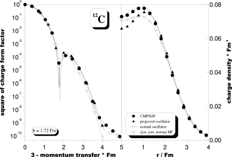
Figure 8: Same as in Fig. 7, but for the nucleus ¹²C.

The energy functional $E_{pr}$ to be used in the Hartree–Fock approach with projection into the COM rest frame before the variation can then be written as

$$E_{pr}\;=\;{{\int da\;a^{2}\int d\Omega_{a}\;h(\vec{a}\,)}\over{\int da\;a^{2}\int d\Omega_{a}\;n(\vec{a}\,)}}$$ (8)

where we have introduced the shifted overlap function

$$n(\vec{a}\,)\;\equiv\;\langle D|\hat{S}(\vec{a}\,)|D\rangle\;=\;{\rm det}X(\vec{a}\,)$$ (9)

which can be represented as the determinant of an $(A\times A)$-matrix

$$X_{hh^{\prime}}(\vec{a}\,)\;\equiv\;\langle h|\hat{S}(\vec{a}\,)|h^{\prime}\rangle\;=\;\sum_{ik}\;D_{ih}S_{ik}(\vec{a}\,)D^{*}_{kh^{\prime}}\noindent$$ (10)

with $S_{ik}(\vec{a}\,)$ being the matrix representation of the shift operator within the chosen harmonic oscillator single particle basis. These matrix elements are given in the appendix A. Furthermore we use in (8) the shifted energy function

$$h(\vec{a}\,)\;\equiv\;\langle D|\hat{H}\hat{S}(\vec{a}\,)|D\rangle\;=\;t(\vec{a}\,)\;+\;v_{2}(\vec{a}\,)$$ (11)

Here the one–body term is given by

$$t(\vec{a}\,)\;=\;n(\vec{a}\,)\;\sum_{ir}\;t(ir)\;\tilde{\rho}_{ri}(\vec{a}\,)\noindent$$ (12)

with the shifted density matrix being defined as

$$\tilde{\rho}_{ri}(\vec{a}\,)\;\equiv\;\sum_{k}\;S_{rk}(\vec{a}\,)\;\sum_{hh^{\prime}}\;D^{*}_{kh}\;[X^{-1}(\vec{a}\,)]_{hh^{\prime}}\;D_{ih^{\prime}}\noindent$$ (13)

and for the two-body part of (11) one obtains

$$v_{2}(\vec{a}\,)\;=\;n(\vec{a}\,)\;{1\over 2}\sum_{ikrs}\;v(ikrs)\;\tilde{\rho}_{sk}(\vec{a}\,)\;\tilde{\rho}_{ri}(\vec{a}\,)$$ (14)

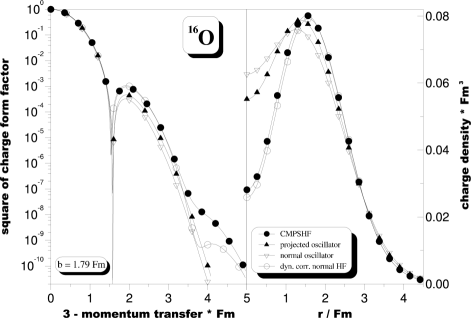
Figure 9: Same as in Fig. 7, but for the nucleus ¹⁶O.

The energy functional (8) has to be minimized with respect to arbitrary variations of the underlying Hartree–Fock transformation $D$. This transformation, however, has to be unitary and thus not all of the $M_{b}\cdot M_{b}$ matrix elements of $D$ are linear independent. Nevertheless an unconstrained minimization of the functional (8) can still be performed, if one parametrizes the underlying Hartree–Fock transformation $D$ via Thouless’ theorem ref15. , which states that any Hartree–Fock determinant $|D_{d}\rangle$ can be represented in terms of the creation and annihilation operators of some reference determinant $|D_{0}\rangle$ via

$$|D_{d}\rangle\;=\;c(d)\exp\left\{\sum_{p,h}\;d_{ph}b^{{\dagger}}_{p}(D_{0})b_{h}(D_{0})\right\}|D_{0}\rangle$$ (15)

provided that the two determinants are non-orthogonal, since

$$c(d)\;=\;\langle D_{0}|D_{d}\rangle$$ (16)

The creation operators belonging to the Hartree–Fock determinant $|D_{d}\rangle$ are then related to those of the reference determinant $|D_{0}\rangle$ via

$$b^{{\dagger}}_{h}(D_{d})\;=\;\sum_{h^{\prime}}[L^{-1}]_{hh^{\prime}}\left(b^{{\dagger}}_{h^{\prime}}(D_{0})\;+\;\sum_{p^{\prime}}\;d_{p^{\prime}h^{\prime}}b^{{\dagger}}_{p^{\prime}}(D_{0})\right)$$ (17)

for the occupied and

$$b^{{\dagger}}_{p}(D_{d})\;=\;\sum_{p^{\prime}}[M^{-1}]_{pp^{\prime}}\left(b^{{\dagger}}_{p^{\prime}}(D_{0})\;-\;\sum_{h^{\prime}}\;d^{*}_{p^{\prime}h^{\prime}}b^{{\dagger}}_{h^{\prime}}(D_{0})\right)$$ (18)

for the unoccupied states, respectively. They are given in terms of the $(M_{b}-A)\cdot A$ linear independent variables $d_{ph}$. The $(A\times A)$ matrix $L$ in (17) is defined by the expression

$${\bf 1}_{A}\;+\;d^{T}d^{*}\;=\;LL^{{\dagger}}$$ (19)

while the $((M_{b}-A)\times(M_{b}-A))$ matrix $M$ out of (18) can be obtained by the solution of the equation

$${\bf 1}_{M_{b}-A}\;+\;d^{*}d^{T}\;=\;MM^{{\dagger}}$$ (20)

The variational equations resulting from the minimization of the functional (8) thus get finally the form

$${{\partial E_{pr}}\over{\partial d_{ph}}}\;=\;\left[{M^{-1}}^{{\dagger}}\;G\;L^{-1}\right]_{ph}\;\equiv\;0$$ (21)

where the $((M_{b}-A)\times A)$ matrix $G$ is defined as

$$G_{ph}\;\equiv\;{{\int da\;a^{2}\int d\Omega_{a}\;g_{ph}(\vec{a}\,)}\over{\int da\;a^{2}\int d\Omega_{a}\;n(\vec{a}\,)}}$$ (22)

and the function $g_{ph}(\vec{a}\,)$ is given by

$$g_{ph}(\vec{a}\,)=\langle D|\;[\hat{H}\;-\;E_{pr}]\;\hat{S}(\vec{a}\,)b^{{\dagger}}_{p}(D)b_{h}(D)\;|D\rangle=$$

$$\sum_{i,r=1}^{M_{b}}\;\sum_{h^{\prime}=1}^{A}\;[X^{-1}(\vec{a}\,)]_{hh^{\prime}}D_{ih^{\prime}}\Biggl{\{}[\;h(\vec{a}\,)\;-\;E_{pr}n(\vec{a}\,)]\;\delta_{ir}+$$

$$n(\vec{a}\,)\sum_{k=1}^{M_{b}}\;\tilde{\Gamma}_{ik}(\vec{a}\,)({\bf 1}\;-\;\tilde{\rho}(\vec{a}\,))_{kr}\Biggr{\}}\sum_{s=1}^{M_{b}}\;S_{rs}(\vec{a}\,)\;D^{*}_{sp}$$

where

$$\tilde{\Gamma}_{ik}(\vec{a}\,)\;\equiv\;t(ik)\;+\;\sum_{rs}\;v(irks)\;\tilde{\rho}_{sr}(\vec{a}\,)$$ (24)

The “local” gradient vector (22), obviously, has to vanish at the solution of (21), too. This solution can be obtained using standard methods as they have been described, e.g., in Ref. ref16. .

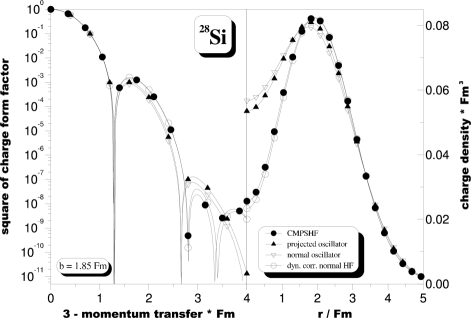
Figure 10: Same as in Fig. 7, but for the nucleus ²⁸Si.

Up to now no symmetry restrictions have been imposed on the Hartree–Fock transformation (3), (4). Thus the Hartree–Fock vacuum (2) breaks in general besides the translational invariance also other symmetries like, e.g., the conservation of the total angular momentum and the parity. For this general case therefore besides the momentum projection also the projection on these other symmetries would be required. The situation becomes, however, much simpler, if only spherically symmetric Hartree–Fock transformations are admitted. Then each of the selfconsistent states created by the operators (3) has the isospin 3-projection, the orbital and total angular momentum and the 3-projection of the latter as “good” quantum numbers, and the sums in (3) and (4) run only over the node quantum number. For nuclei with closed angular momentum subshells the corresponding Hartree–Fock vacuum (2) has then total angular momentum $I^{\pi}=0^{+}$ and conserves the proton as well as the neutron number. Consequently the projection on these symmetries becomes redundant and we are left with only the linear momentum projection as described above.

Furthermore, for spherically symmetric systems obviously neither the shifted overlap (9) nor the corresponding energy function (11) do depend on the direction of the shift vector $\vec{a}$. Thus the angle integrations in (8) and (21) induced by the operator (6) become trivial and only a single integral over the radial component of the shift vector remains to be done numerically. An explicit formulation of this special case will not be given in the present paper. However, it is obvious that the calculation of the expressions needed for the minimization of the energy functional (8) is then simplified considerably.

3 Results and discussion.

We have considered the six nuclei ⁴He, ¹²C, ¹⁶O, ²⁸Si, ³²S and ⁴⁰Ca. As hamiltonian, as in ref. ref12. , the Brink–Boeker interaction B1 ref14. complemented with a short range (0.5 Fm) two–body spin–orbit term having the same volume–integral as the corresponding zero–range term of the Gogny–force D1S ref17. , plus the Coulomb force and the kinetic energy has been used. First, the energy of the simple oscillator determinants for these nuclei (e.g., $(0s)^{4}(0p)^{12}$ for ¹⁶O) has been minimized with respect to the oscillator length–parameter $b$. For the intermediate states needed to compute the shifted energy function (11) here four major shells more than in the basis have been taken (e.g., in ¹⁶O the maximum $N=2n+l$ of the oscillator determinant is 1. Hence, for the intermediate states all orbits up to N=5 have been used). The results obtained were identical to those obtained analytically in ref. ref12. , which is a good check of the convergence of the numerical procedure.

In the next step then, for increasing size of the single particle basis up to $N=2n+l=18$, in each nucleus and each basis system always three different Hartree–Fock calculations have been performed :

First, a usual spherical Hartree–Fock calculation was done, in which the energy

$$E^{\prime}_{n}\;=\;\langle D_{n}|\hat{H}|D_{n}\rangle$$ (25)

is minimized and after convergence corrected by subtracting the expectation value of the kinetic energy of center of mass motion

$$E_{n}\;=\;E^{\prime}_{n}\;-\;\langle D_{n}|{{{\hat{P}\,}^{2}}\over{2MA}}|D_{n}\rangle$$ (26)

This is the normal approach as indicated by the subscripts $n$ at the total energy and the wave function.

Second, a corrected spherical Hartree–Fock calculation has been done, in which the expectation value of the internal hamiltonian

$$E_{c}\;=\;\langle D_{c}|\left(\hat{H}\,-\,{{{\hat{P}\,}^{2}}\over{2MA}}\right)|D_{c}\rangle$$ (27)

is minimized. The subscript $c$ refers to this corrected approach.

Figure 11: Same as in Fig. 7, but for the nucleus ³²S.

Third, a spherical Hartree–Fock calculation with projection into the center of mass rest frame before the variation as described in section 2 has been performed. In this case the energy–functional (8)

$$E_{pr}\;=\;{{\langle D_{pr}|\hat{H}\,\hat{C}(0)|D_{pr}\rangle}\over{\langle D_{pr}|\hat{C}(0)|D_{pr}\rangle}}$$ (28)

has been minimized. Here, for the intermediate states again always four major shells more than for the basis have been taken into account. Note, that $|D_{n}\rangle$, $|D_{c}\rangle$ and $|D_{pr}\rangle$ result from different variational calculations and are hence different.

Finally, for the largest basis system ($N=18$), we have studied in each nucleus a widely used approximate description to deal with the center of mass motion : instead of minimizing $E_{c}$ out of equation (27) one minimizes

$$E^{\prime}_{\lambda}\;=\;\langle D_{\lambda}|\left(\hat{H}\,-\,{{{\hat{P}\,}^{2}}\over{2MA}}\right)|D_{\lambda}\rangle\,+$$

$$+\,\lambda\,\cdot\,\langle D_{\lambda}|\left({{{\hat{P}\,}^{2}}\over{2MA}}\,+\,{1\over 2}MA\omega^{2}{\vec{R}\,}^{2}\right)|D_{\lambda}\rangle$$ (29)

with a large Lagrangian multiplier $\lambda$, i.e., one penalizes center of mass excitations. This prescription is exact for so called complete $n\hbar\omega$ configuration spaces ref2. , however, is often applied also in truncated shell–model spaces [18,19]. The internal energy (i.e., (3) without the penalizing term) has been obtained for the three different $\lambda$ values 10, 100 and 10000.

In addition, again always for the largest basis, the hole–energies obtained for the corrected approach

$$E^{h}_{c}\;=\;E_{c}\,-\,\langle D_{c}|b_{h}^{\dagger}(D_{c})\left(\hat{H}\,-\,{{{\hat{P}\,}^{2}}\over{2M(A-1)}}\right)b_{h}(D_{c})|D_{c}\rangle$$ (30)

have been compared with the projected results

$$E^{h}_{pr}\;=\;E_{pr}\,-\,{{\langle D_{pr}|b_{h}^{\dagger}(D_{pr})\hat{H}\hat{C}(0)b_{h}(D_{pr})|D_{pr}\rangle}\over{\langle D_{pr}|b_{h}^{\dagger}(D_{pr})\hat{C}(0)b_{h}(D_{pr})|D_{pr}\rangle}}$$ (31)

as well as the corresponding results for the simple oscillator occupations. For the nuclei, in which two s–states are occupied (³²S and ⁴⁰Ca), obviously an additional diagonalization has been performed.

Note, that the definition (30) differs from the usual expression since via the kinetic energy of the center of mass motion the internal hamiltonian becomes A–dependent. The resulting difference with respect to the usual expression is for non–spurious oscillator hole–states $3\hbar\omega/4(A-1)$ and in the general case always larger than this lower limit. Inserting the results for $\hbar\omega$ into this formula, one obtains considerable effects even for the larger A-values considered here.

The results for the total binding energies and the hole-energies of the considered nuclei are summerized in figures 1 to 6. The left side of each figure presents the total binding energy as function of the size of the basis. Three different curves are plotted : open circles refer to the Hartree–Fock results (26) where the kinetic energy of the center of mass motion is subtracted after the variation, full triangles give the results of the corrected approach (27), in which this subtraction is done before the variation and full circles display the results of the spherical Hartree–Fock calculations with projection into center of mass rest frame before the variation (28).

For pure oscillator occupations (i.e., the smallest basis) these three curves obviously coincide, for larger basis systems, however, they differ considerably, i.e., display rather different major–shell–mixing. Let us first concentrate on the unprojected approaches (26) and (27). As expected, the corrected approach (27) yields always a lower binding energy than the normal one (26), however, for all but one of the considered nuclei the corresponding curves run almost parallel with increasing basis size and their difference is rather small. The exception is the case of ⁴He, where (26) even yields a decrease in binding energy with the basis size such indicating that the underlying wave functions have a rather different structure than those obtained via (27). The energy gain of the projected approach (28) with respect to the corrected prescription (27) is in all considered nuclei (except ⁴He) much larger than that of the latter with respect to (26). For ⁴⁰Ca in the largest basis system, e.g., the projected binding energy is 1.25 MeV lower than the corrected result, while the latter is only 136 keV lower than the normal one. Note, that these 1.25 MeV amount to almost 20 percent of the total major shell mixing obtained in the corrected approach (27). Thus, obviously, the restoration of Galilean invariance yields a considerable effect on the total binding energy and should not be neglected even for nuclei as heavy as ⁴⁰Ca.

Furthermore, as can be seen from the inverted triangles in the figures, the prescription (3), which penalizes center of mass excitations, fails completely. For the largest Lagrange multiplier ($\lambda=10000$) the procedure yields in all considered nuclei just the simple oscillator occupation. This, definitely, is a non–spurious state (i.e., contains no center of mass excitations), however, the major–shell–mixing is completely supressed in this solution. This is a severe warning to use the prescription (3) in incomplete model spaces : it always prefers non–spurious (one valence shell) solutions and is hence uncontrollable even if the configuration space is less severly truncated as in the simple Hartree–Fock approach discussed here.

On the right side of figures 1 to 6 we display the proton and neutron hole–energies in the considered nuclei. Always the corrected results (30) (indicated by the label no) are compared with the projected energies (31) (indicated by the label pr) for both the oscillator occupation (HO) as well as the Hartree-Fock approach (HF) calculated in the $N=18$ basis.

Though the underlying wave functions (and total binding energies) are considerably different, in all considered nuclei the harmonic oscillator approach and the Hartree–Fock method yield remarkably similar results. For the non–spurious hole–states out of the last occupied major shell in the harmonic oscillator approach the corrected and projected results have to be identical as demonstrated analytically in ref. ref12. and this feature holds to a large extent for the Hartree–Fock results, too. For the hole–states out of the second and third but last occupied shell corrected and projected results display in both approaches rather similar pronounced differences. So, e.g., in ¹⁶O the projected p–holes are more than 6 MeV lower in energy than the corresponding corrected results and even in ⁴⁰Ca the differences are still about 2.5 MeV for both the p– and the lowest s–holes. It was demonstrated in ref.ref12. that these differences are consistent with the differences in the spectroscopic factors out of ref.ref10. . This will be discussed in more detail in the second of the present series of papers.

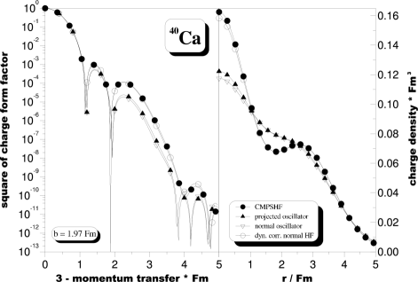
Figure 12: Same as in Fig. 7, but for the nucleus ⁴⁰Ca.

An interesting observation is made for the two nuclei ²⁸Si and ³²S. Here, the p1/2–holes are almost unaffected by the projection, while the p3/2–holes show the same differences as, e.g., observed in ⁴⁰Ca. Since the coupling of p1/2 and d5/2 to angular momentum one is not possible and the d3/2–orbit is unoccupied in these two nuclei, this observation points to the dominance of angular momentum one couplings for the hole energies.

The figures 7 to 12 demonstrate the effects on the charge form factors and corresponding charge densities. Usually, the operator for the charge density in momentum representation is written as ref20. ; ref11.

$$\hat{\rho}_{n}\,\equiv\,\sum_{\tau}f_{\tau}(Q^{2})\,\sum_{i=1}^{N_{\tau}}\,\exp\{i\vec{q}\cdot\vec{r}_{i}\}$$ (32)

where $\tau$ is the isospin projection (proton or neutron) and the nucleon charge form factors $f_{\tau}$ are given by

$$f_{\tau}(Q^{2})\,\equiv\,G^{\tau}_{E}(Q^{2})\,-\,{{Q^{2}}\over{8M^{2}}}\,{{G^{\tau}_{E}(Q^{2})\,+\,{{Q^{2}}\over{4M^{2}}}\,G^{\tau}_{M}(Q^{2})}\over{1\,+\,{{Q^{2}}\over{4M^{2}}}}}$$ (33)

with the Sachs–form factors parametrized in the well–known dipole form (see, e.g., ref21. )

$$G^{p}_{E}(Q^{2})\,\equiv\,\left[1\,+\,{{Q^{2}}\over{(843{\rm MeV})^{2}}}\right]^{-2}$$

$$G^{\tau}_{M}(Q^{2})\,\equiv\,\mu_{\tau}\,G^{p}_{E}(Q^{2})$$

$$\mu_{p}\,=+2.793$$

$$\mu_{n}\,=-1.913$$

$$G^{n}_{E}(Q^{2})\,\equiv\,-\mu_{n}\,{{Q^{2}}\over{4M^{2}}}\,{1\over{1\,+\,5.6{{Q^{2}}\over{4M^{2}}}}}\,G^{p}_{E}(Q^{2})$$ (34)

Here $M$ is the nucleon mass and $Q^{2}$ the negative square of the 4–momentum transfer

$$Q^{2}\,\equiv\,(\hbar c\vec{q}\,)^{2}\,-\,(\Delta E)^{2}\noindent$$ (35)

with $\Delta E$ being the energy transfer and $\vec{q}$ the 3–momentum transfer to the system. For elastic electron scattering the energy transfer is given by the recoil energy $(\hbar c\vec{q}\,)^{2}/(2AMc^{2})$ so that here

$$Q^{2}\,=\,(\hbar c\vec{q}\,)^{2}\left\{1\,-\,{{(\hbar c\vec{q}\,)^{2}}\over{4A^{2}M^{2}c^{4}}}\right\}$$ (36)

If, as in our case, the ground state is described by a single determinant $|D\rangle$, then the “normal” elastic charge form factor has the form

$$F_{ch}^{n}(Q^{2})\,=\,\langle D|\hat{\rho}_{n}|D\rangle$$ (37)

and the corresponding charge density is just the Fourier–transform of this expression.

Obviously, to obtain a translational invariant form for the charge density operator, (32) has to be complemented with the so–called Gartenhaus–Schwartz operator as has been demonstrated in ref. ref11.

$$\hat{\rho}_{inv}\,\equiv\,\hat{\rho}_{n}\,\exp\{-i\vec{q}\cdot\vec{R}\}$$ (38)

The Galilei–invariant form of the charge form factor is thus

$$F_{ch}^{pr}(Q^{2})\,=\,{{\langle D|\hat{\rho}_{inv}\hat{C}(0)|D\rangle}\over{\langle D|\hat{C}(0)|D\rangle}}\noindent$$ (39)

The matrix elements needed to compute this expression are given in appendix B. The corresponding charge density is then again obtained by Fourier–transforming this expression.

It has been demonstrated already some time ago ref8. that using the so–called Gaussian–overlap–approximation for both the shift as well as for the Gartenhaus–Schwartz operator (38) reduces to the “dynamically corrected” charge form factor

$$F_{ch}^{dy}(Q^{2})\,=\,F_{ch}^{n}(Q^{2})\,\exp\left\{{3\over 8}\,{{{\vec{q}\,}^{2}}\over{\langle D|{\hat{P}\,}^{2}|D\rangle}}\right\}\noindent$$ (40)

In case that $|D\rangle$ is a non–spurious oscillator state the exponential factor in (40) gets the form $\exp\{(\vec{q}\,b/2)^{2}/A\}$, which is the famous Tassie–Barker correction [5].

On the left side of the figures 7 to 12 we compare for the considered nuclei the normal form factor (37) for the oscillator occupation (inverted open triangles) with the corresponding projected one (39) (full triangles), the dynamically corrected one (40), resulting from the solution $|D_{c}\rangle$ of the minimization of the Hartree–Fock energy functional (27), and, finally, the Galilei–invariant one (38) computed from the solution $|D_{pr}\rangle$ of the minimization of the projected energy functional (28) (full circles). The corresponding charge densities are given on the right side of the figures. All Hartree–Fock results have been obtained using the largest basis with 19 major oscillator shells.

Let us first concentrate on the oscillator occupation. In ⁴He a large difference between the normal and the projected oscillator form factors at high momentum transfer and consequently for the charge density at small radii is observed. Since we have here a non–spurious oscillator state this difference is entirely due to the Tassie–Barker correction. This correction decreases with increasing mass number and can in ⁴⁰Ca almost be neglected. On the other hand the difference of the Hartree–Fock results with respect to the oscillator ones increase with increasing mass number due to the increasing major shell mixing. E.g., in ⁴⁰Ca Hartree–Fock and oscillator results look rather different.

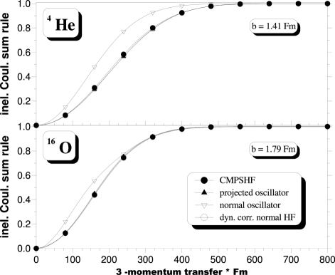
Figure 13: The inelastic (mathematical) Coulomb sum rule as function of the 3–momentum transfer. Compared are the results of calculations using an oscillator occupation and an uncorrected elastic charge form factor (for point protons) with those using the same occupation but including the Tassie–Barker factor for the elastic charge form factor, those of a normal Hartree–Fock calculation including the dynamical correction for the elastic charge form factor and, finally, those of the projected CMPSHF approach. The upper part of the figure gives the results for ⁴He, the lower part those for the nucleus ¹⁶O.

Though computed with rather different wave functions the projected and dynamically corrected form factors and charge densities display only rather small differences in all the considered nuclei except ⁴He. This is somewhat surprising since in ref. ref7. ; ref8. larger effects of the projection have been seen even for nuclei up to A=40. However, besides being limited to projection after the variation, these calculations had been done with different effective interactions than used in the present work. Thus the present results do not indicate that for the elastic form factors and charge densities the dynamical correction is good enough and no projection is needed. Instead a more careful study using various effective interactions is required.

In addition to the form factors we have studied the mathematical Coulomb sum rules, too. Details of its definition can be found in ref. ref11. . As usual we assumed point nucleons, i.e., we set the nucleon form factors out of eq. (33) to 1 for the proton and 0 for the neutron. Furthermore, again as usual, we subtracted the square of the elastic form factor and divided the result by the charge number in order to obtain the so–called inelastic Coulomb sum rules. Without any center of mass correction these have the form

$$\Sigma^{inel,\,n}(q)\,=\,{1\over Z}\,\left\{\langle D_{n}|\hat{\rho}_{n}{\hat{\rho}_{n}\,}^{{\dagger}}|D_{n}\rangle\,-\,\left(F_{ch}^{n}(q)\right)^{2}\right\}$$ (41)

where the elastic form factor out of eq. (37) has to be taken in the point proton limit. If we include the dynamical correction for the elastic form factor we obtain the result

$$\Sigma^{inel,\,dy}(q)\,=\,{1\over Z}\,\left\{\langle D_{c}|\hat{\rho}_{n}{\hat{\rho}_{n}\,}^{{\dagger}}|D_{c}\rangle\,-\,\left(F_{ch}^{dy}(q)\right)^{2}\right\}\noindent$$ (42)

with the point proton limit for expression (40), and, finally, the linear momentum projected expression has the form

$$\Sigma^{inel,\,pr}(q)\,=\,{1\over Z}\,\left\{{{\langle D_{pr}|\hat{\rho}_{n}{\hat{\rho}_{n}\,}^{{\dagger}}\hat{C}(0)|D_{pr}\rangle}\over{\langle D_{pr}|\hat{C}(0)|D_{pr}\rangle}}\,-\,\left(F_{ch}^{pr}(q)\right)^{2}\right\}$$ (43)

with the point proton limit of the form factor (39). Explicit forms for the matrix elements entering the expressions (41-43) are for spherically symmetric determinants $|D\rangle$ given in appendix C. Note, that it is irrelevant whether in the first term of these expression the normal (32) or the invariant form (38) of the charge density operator is used, since in these matrix elements the Gartenhaus–Schwartz operator does drop out. As for the charge form factors and densities the normal (41) and projected (43) results for the oscillator occupation have been compared with the dynamically corrected (42) and the projected (43) Hartree–Fock results. For the computation of the latter obviously again the solutions $|D_{c}\rangle$ and $|D_{pr}\rangle$ of the corresponding variational calculations have been taken.

The results for ⁴He and ¹⁶O are displayed in figure 13. Plotted are the inelastic sum rules as defined above as functions of the 3–momentum transfer $q$. As expected from the similarity of the dynamically corrected and the projected elastic Hartree–Fock form factors almost no differences between these two approaches are obtained for the inelastic sum rules either. That the projected oscillator results almost coincide with the Hartree–Fock results, too, is a clear indication that the inelastic sum rule is rather insensitive to the major shell mixing. However, all these results approach the limit of 1 considerably slower than the normal oscillator approach. This difference is entirely due to the square of the elastic form factor in the above expressions and demonstrates that a correct treatment of the latter (either exact by projection or approximate by the dynamical correction) is definitely required.

Since for the inelastic sum rules of the other considered nuclei the same behaviour as demonstrated in figure 13 is obtained, we shall not discuss them here.

4 Conclusions.

We have presented the total binding energies, hole energies, form factors and charge densities as they result from spherical Hartree–Fock calculations with projection into the center of mass rest frame before the variation for the six nuclei ⁴He, ¹²C, ¹⁶O, ²⁸Si, ³²S and ⁴⁰Ca and have compared them to the standard Hartree–Fock results obtained by subtracting the kinetic energy of the center of mass motion either after or before the variation. Furthermore, for the two nuclei ⁴He and ¹⁶O, we have discussed the inelastic Coulomb sum rule resulting from these different approaches. For comparison, in addition the results for pure oscillator occupations have been discussed.

For the total binding energies considerable effects of the correct treatment of Galilei–invariance are seen. In all the considered nuclei the energy gains of the momentum projected solutions with respect to the conventionally corrected approach using just the internal hamiltonian (which contains already the usual 1/A effect) in the variation are a considerable portion of the gains due to major shell mixing and hence as important as the latter. It was furthermore demonstrated that the often used approximate prescription to penalize center of mass excitations by an additional term in the variation does not work at all at least in the severly truncated configuration spaces used here. There are strong indications that this prescription does only work in complete $n\hbar\omega$–spaces and is uncontrollable even if used in less severly truncated shell–model spaces.

For the hole energies essentially the same features as in ref. ref12. are observed. While the energies of the holes out of the last occupied shell are almost unaffected, the projected energies of the holes out of the second and third but last shell are considerably different from their conventionally corrected counterparts (which again include the trivial 1/A effects).

For the elastic charge form factors and densities (except for the lightest considered system) there are little differences obtained between the projected and the dynamically corrected approach though these two approaches use rather different wave functions resulting from different variational calculations and the same holds for the inelastic Coulomb sum rules. However, these results may be changed, if a different (more realistic) effective interaction is used, and hence have to be interpreted with some care.

In conclusion, it has been demonstrated that a correct treatment of Galilei–invariance in the nuclear many–body problem is possible via projection methods and that its effects are not only important for simple harmonic oscillator configurations as shown in refs. ref10. ; ref11. ; ref12. ; ref13. but also for more realistic wave functions. We shall show in the second of these two papers that this holds also for the spectral functions and spectroscopic factors. Thus we think that the (up to now mostly neglected) restoration of Galilei–invariance is unavoidable in future nuclear structure calculations, and, on the long run, should also be done in more sophisticated approaches like the shell–model [18], the quantum Monte–Carlo diagonalization method ref19. or the VAMPIR approach ref22. .

5 Appendix A: Oscillator matrix elements of the shift operator.

The single particle matrix elements $S_{ik}(\vec{a}\,)$ (10) of the shift operator (7) within oscillator single particle states play an essential role in the projected formalism presented in section 2. They have been given already in ref. ref6. . Using the usual quantum numbers $\tau$, $n$, $l$, $j$ and $m$ for the isospin projection, the node number (starting from zero), the orbital angular momentum $l$, which is coupled with the spin to the total angular momentum $j$ and its 3–projection $m$, we obtain

$$\langle\tau_{1}n_{1}l_{1}j_{1}m_{1}|\hat{S}(\vec{a}\,)|\tau_{2}n_{2}l_{2}j_{2}m_{2}\rangle=\delta_{\tau_{1}\tau_{2}}\exp\left\{-{1\over 4}\alpha^{2}\right\}$$

$$\times\sum_{L}\sqrt{{{4\pi}\over{2L+1}}}\,Y^{*}_{L\Lambda}(\Omega_{a})\,{1\over 2}\left[1\,+\,(-)^{l_{1}+l_{2}+L}\right]$$

$$\times(-)^{[L+l_{2}-l_{1}]/2}\sqrt{(2j_{1}+1)(2j_{2}+1)}(-)^{j_{1}-1/2}$$

$$\times(j_{1}j_{2}L|1/2-1/20)(-)^{j_{2}-m_{2}}$$

$$\times(j_{1}j_{2}L|m_{1}-m_{2}\Lambda)\,\eta_{L}^{n_{1}l_{1}n_{2}l_{2}}(\alpha)$$

where $\alpha\,=\,|\vec{a}\,|/b$ with $b$ being the oscillator length and

$$\eta_{L}^{n_{1}l_{1}n_{2}l_{2}}(\alpha)=\exp\left\{+{1\over 4}\alpha^{2}\right\}(-)^{n_{1}+n_{2}}\int\limits_{0}^{\infty}d\kappa\,{\rm e}^{-\kappa^{2}}$$

$$\times\kappa^{2}\,\tilde{R}_{n_{1}l_{1}}(\kappa)\,j_{L}(\kappa\alpha)\,\tilde{R}_{n_{2}l_{2}}(\kappa)$$ (45)

where $\tilde{R}_{nl}(\kappa)$ are the (dimensionless) polynomial parts of the usual spherical radial oscillator functions depending on the dimensionless variable $\kappa$. An analytical form of the expression (5) has been given in ref. ref6. and will not be repeated here.

In case that the shift vector can be put in z–direction as in the spherically symmetric systems considered here, then

$$\sqrt{{{4\pi}\over{2L+1}}}\,Y^{*}_{L\Lambda}(\hat{z})\,\equiv\,\delta_{\Lambda 0}$$ (46)

Then, in eq. (5), obviously, $m_{1}$ and $m_{2}$ have to be equal and the evaluation of the formulas in section 2 is simplified considerably.

6 Appendix B:The projected charge form factor.

In this appendix we shall give the formulas needed to evaluate the projected charge form factor out of eq. (39). Again we assume that the determinant $|D\rangle$ is spherical symmetric. This allows to fix the direction of the momentum transfer to the z–axis. Furthermore it can be shown easily, that the dependence on the angle $\varphi_{a}$ of the shift vector is is trivial and can be integrated out analytically. Left to be done is then a two–fold integration over the length of the shift vector and over the angle $\vartheta_{a}$ between the shift vector and the z–axis (direction of the momentum transfer). After some tedious but straightforward calculation we obtain

$$F^{pr}_{ch}(Q^{2})={{4\pi b^{3}}\over{\langle D|\hat{C}(0)|D\rangle}}\exp\left\{-{{A-1}\over{A}}\left({{bq}\over{2}}\right)^{2}\right\}$$

$$\int_{0}^{\infty}d\alpha\alpha^{2}\exp\left\{-{{A}\over{4}}\alpha^{2}\right\}\int_{0}^{\pi/2}d\vartheta_{a}\sin\vartheta_{a}$$

$$\cdot\,2{\rm Re}\Biggl{\{}\Bigl{[}\prod\limits_{\tau=p,n}{\rm det}z^{\tau}(bq,\,\alpha,\,\vartheta)\Bigr{]}\Bigl{[}\sum\limits_{\tau}f_{\tau}(Q^{2})$$

$${\sum\limits_{h_{1},h_{2}>0}}^{(\tau)}\Bigl{\{}\qquad\;\;\;\,y^{\tau}_{h_{1}h_{2}}(bq,\,\alpha,\,\vartheta){z^{\tau}}^{-1}_{h_{2}h_{1}}(bq,\,\alpha,\,\vartheta)$$

$$\qquad-\,y^{\tau}_{h_{1}{\bar{h}}_{2}}(bq,\,\alpha,\,\vartheta){z^{\tau}}^{-1}_{h_{2}{\bar{h}}_{1}}(bq,\,\alpha,\,\vartheta)\Bigr{\}}\Bigr{]}\Biggr{\}}$$

where $b$ is again the oscillator length, $\alpha\,=\,|\vec{a}\,|/b$, and $\bar{h}$ denotes the time reversed partner of the hole state $h$. The second sum in eq. (6) is restricted to positive values of the 3–projections of the two hole states. Furthermore $\vec{q}$ denotes the 3–momentum transfer while $Q^{2}$ is the (negative) square of the 4–momentum transfer as in section 2. The nucleon form factors $f_{\tau}(Q^{2})$ are given by eq. (33). Furthermore

$$z^{\tau}_{12}(bq,\,\alpha,\,\vartheta)=\sum\limits_{L}\sqrt{(2j_{1}+1)(2j_{2}+1)}(-)^{j_{2}-m_{2}}$$

$$(j_{1}j_{2}L|m_{1}-m_{2}\Lambda)(-)^{j_{1}-1/2}(j_{1}j_{2}L|1/2-1/20)$$

$$\Biggl{\{}{{\sqrt{2L+1}}\over{(l_{1}l_{2}L|000)}}{1\over 2}\left[1+(-)^{l_{1}+l_{2}+L}\right]-{{\sqrt{2L+1}}\over{(l_{1}l_{2}L|1-10)}}\times$$

$$\times{1\over 2}\left[1-(-)^{l_{1}+l_{2}+L}\right]\,{{L(L+1)-\kappa_{12}(\kappa_{12}+1)}\over{2\sqrt{l_{1}(l_{1}+1)l_{2}(l_{2}+1)}}}\Biggr{\}}$$

$$\sum\limits_{L_{1}L_{2}l}(LL_{2}L_{1}|\Lambda-\Lambda 0)d^{L_{2}}_{\Lambda 0}(\vartheta_{a})\,i^{L_{1}}\,(-)^{[l+l_{2}-L_{2}]/2}$$

$$\sum\limits_{n}(-)^{n_{1}+n}\eta_{L_{1}}^{n_{1}l_{1}nl}(qb/A)\eta_{L_{2}}^{nln_{2}l_{2}}(\alpha)\sqrt{{{(2L_{1}+1)(2L_{2}+1)}\over{2l_{2}+1}}}$$

$$(l_{1}L_{1}l|000)\Bigl{\{}(l_{1}Ll_{2}|000)(l_{1}L_{1}l|000)(LL_{1}L_{2}|000)$$

$$+2\sum\limits_{\lambda=1}^{{\rm min}(l_{1},L,L_{1})}(-)^{\lambda}(l_{1}Ll_{2}|\lambda-\lambda 0)$$

$$(l_{1}L_{1}l|\lambda-\lambda 0)(LL_{1}L_{2}|\lambda-\lambda 0)\Bigr{\}}$$

where the $\eta$’s are given by expression (5) and

$$\kappa_{12}\,\equiv\,(l_{1}-j_{1})(2j_{1}+1)+(l_{2}-j_{2})(2j_{2}+1)$$ (49)

The matrix elements of $y^{\tau}_{12}$ have exactly the same form as (6) except that the imaginary unit $i$ has to be replaced by $-i$ and the argument in the first $\eta$ has to be multiplied with a factor $(A-1)$. Note, that the expression (6) includes both natural and unnatural parity terms in the sum over $L$. The latter had been neglected in ref. ref8. .

7 Appendix C:The mathematical Coulomb sum rule.

In this appendix we give the explicit formulas for the matrix elements entering expressions (41-43) for the inelastic Coulomb sum rules. In the normal approach one obtains for spherically symmetric Hartree–Fock transformations

$$\Sigma_{0}^{nor}(q)=\langle D|{\hat{\rho}}_{n}{\hat{\rho}}_{n}^{\dagger}|D\rangle=\,Z\,+\,\exp\left\{-{1\over 2}(bq)^{2}\right\}$$

$$\Biggl{\{}\Bigl{[}{\sum\limits_{\alpha_{h}l_{h}j_{h}}}^{(p)}(2j_{h}+1)\chi_{0}^{\alpha_{h}l_{h};\,\alpha_{h}l_{h}}(qb)\Bigr{]}^{2}$$

$$-\,{\sum\limits_{\alpha_{h}l_{h}j_{h}}}^{(p)}{\sum\limits_{\alpha_{h^{\prime}}l_{h^{\prime}}j_{h^{\prime}}}}^{(p)}\sum\limits_{L}\,{1\over 2}\Bigl{[}1+(-)^{l_{h}+l_{h^{\prime}}+L}\Bigr{]}$$

$$\Delta(l_{h},\,l_{h^{\prime}},\,L)(j_{h}j_{h^{\prime}}L|1/2-1/20)^{2}$$

$$(2j_{h}+1)(2j_{h^{\prime}}+1)\Bigl{(}\chi_{L}^{\alpha_{h}l_{h};\,\alpha_{h^{\prime}}l_{h^{\prime}}}(qb)\Bigr{)}^{2}\Biggr{\}}$$

where $\Delta(l_{h},\,l_{h^{\prime}},\,L)=1$ if $|\,l_{h}-l_{h^{\prime}}|\leq L\leq l_{h}+l_{h^{\prime}}$ and $=0$ else,

$$\chi_{L}^{\alpha_{h}l_{h};\,\alpha_{h^{\prime}}l_{h^{\prime}}}(qb)={\sum\limits_{n}}^{(l_{h}j_{h})}{\sum\limits_{n^{\prime}}}^{(l_{h^{\prime}}j_{h^{\prime}})}\,D_{n\alpha_{h}}^{p\,l_{h}j_{h}}$$

$$(-)^{n+n^{\prime}}\eta_{L}^{nl_{h}n^{\prime}l_{h^{\prime}}}(qb)D_{n^{\prime}\alpha_{h^{\prime}}}^{p\,l_{h^{\prime}}j_{h^{\prime}}},\noindent$$ (51)

and the $\eta$’s are given by the expression (5).

In order to evaluate the corresponding Galilei–invariant expression for spherically symmetric determinants $|D\rangle$ the shift vector can again be put in z–direction. We obtain

$$\Sigma_{0}^{proj}(q)={{\langle D|{\hat{\rho}}_{n}{\hat{\rho}}_{n}^{\dagger}\hat{C}(0)|D\rangle}\over{\langle D|\hat{C}(0)|D\rangle}}=\,Z\,+\,\exp\left\{-{1\over 2}(bq)^{2}\right\}$$

$${\langle D|\hat{C}(0)|D\rangle}^{-1}\,4\pi b^{3}\,\int\limits_{0}^{\infty}d\alpha\,\alpha^{2}\langle D|\hat{S}(\hat{e}_{z}\cdot\vec{a}\,)|D\rangle$$

$$\Biggl{\{}\sum\limits_{L}{1\over{2L+1}}\Biggl{(}{\sum\limits_{AC}}^{(p)}M_{AC}^{L}(qb)\,\tilde{\rho}_{CA}^{L}(\alpha)\Biggr{)}^{2}$$

$$-\,{\sum\limits_{ABCD}}^{(p)}\sum\limits_{L}\Biggl{(}\sum\limits_{I}(-)^{I-L+1}\left\{\matrix{j_{A}&j_{C}&L\cr j_{B}&j_{D}&I\cr}\right\}$$

$$M_{AD}^{I}(qb)M_{BC}^{I}(qb)\Biggr{)}{\tilde{\rho}}_{CA}^{L}(\alpha){\tilde{\rho}}_{DB}^{L}(\alpha)\Biggr{\}}$$

where $A,\,B$,… denote the quantum numbers of the oscillator single particle basis states $n_{A}l_{A}j_{A},\,n_{B}l_{B}j_{B}$,…, $\vec{\alpha}\,=\,\vec{a}/b$ with $b$ being the oscillator length parameter, and

$$M_{AC}^{L}(qb)={1\over 2}\left[1+(-)^{l_{A}+l_{C}+L}\right]\Delta(l_{A},\,l_{C},\,L)$$

$$\sqrt{(2j_{A}+1)(2j_{C}+1)}(-)^{j_{A}-1/2}(j_{A}j_{C}L|1/2-1/20)$$

$$(-)^{n_{A}+n_{C}}\,\eta_{L}^{n_{A}l_{A}n_{C}l_{C}}(qb)$$

are the reduced oscillator single particle matrix elements of the normal charge density operator in momentum representation. The supersript $(p)$ at the sum symbols means that only proton–orbits are considered. Finally,

$${\tilde{\rho}}_{CA}^{L}(\alpha)\,\equiv\,\sum\limits_{m}(-)^{j_{C}-m}(j_{A}j_{C}L|m-m0)\,{\tilde{\rho}}_{CA}^{(m)}(\alpha)$$ (54)

where

$${\tilde{\rho}}_{CA}^{(m)}(\alpha)={\sum\limits_{HH^{\prime}}}^{(p)}\,S_{CH}^{(pm)}(\alpha){S_{HH^{\prime}}^{(pm)}}^{-1}(\alpha)$$

$$D_{n_{A}\alpha_{H^{\prime}}}^{(p\,l_{A}j_{A})}\,\delta_{l_{H^{\prime}}l_{A}}\delta_{j_{H^{\prime}}j_{A}}$$ (55)

In eq. ( 7) use has been made of the fact, that the single particle matrix elements do not mix different isospin projections, and, for the shift vector in z–direction, do not mix states with different total angular momentum projections $m$ either. This is indicated by the superscipts $(pm)$.

References

- (1) J.P. Elliot, T.H.R. Skyrme, Proc. Roy. Soc. A 232, 561 (1955).
- (2) B. Giraud, Nucl. Phys 71, 373 (1965).
- (3) R.E. Peierls, J. Yoccoz, Proc. Phys. Soc. London Ser. A 70, 381 (1957); R.E. Peierls, D.J. Thouless, Nucl. Phys. 38, 154 (1962); J. Yoccoz, Proceedings of the International School of Physics “Enrico Fermi”, Course XXXVI, edited by C. Bloch (Academic Press, 1966) p. 474.
- (4) P. Ring, P. Schuck, The Nuclear Many–body Problem (Springer, Berlin–Heidelberg–New York, 1980).
- (5) L.J. Tassie, C.F. Barker, Phys. Rev. 111, 940 (1958).
- (6) K.W. Schmid, F. Grümmer, Z. Phys. A 336, 5 (1990).
- (7) K.W. Schmid, F. Grümmer, Z. Phys. A 337, 267 (1990).
- (8) K.W. Schmid, P.–G. Reinhard, Nucl. Phys. A 530, 283 (1991).
- (9) K.W. Schmid, G. Schmidt, Prog. Nucl. Part. Phys. 34, 361 (1995).
- (10) K.W. Schmid, Eur. Phys. J. A 12, 29 (2001).
- (11) K.W. Schmid, Eur. Phys. J. A 13, 319 (2002).
- (12) K.W. Schmid, Eur. Phys. J. A 14, 413 (2002).
- (13) K.W. Schmid, Eur. Phys. J. A 16, (2003), in press.
- (14) D.M. Brink, E. Boeker, Nucl. Phys. A 91, 1 (1966).
- (15) D.J. Thouless, Nucl. Phys. 21, 225 (1960).
- (16) K.W. Brodlie, The state of the art in numerical analysis, edited by D. Jacobs (Academic, New York 1977) p. 229.
- (17) J.F. Berger, M. Girod, D. Gogny, Comp. Phys. Commun. 63, 365 (1991).
- (18) B.A. Brown, Prog. Part. Nucl. Phys. 47, 517 (2001).
- (19) T. Otsuka, M. Homma, T. Mizusaki, N. Shimizu, Y. Utsuno, Prog. Part. Nucl. Phys. 47, 319 (2001).
- (20) T.W. Donelly, W.C. Haxton, At. Data Nucl. Data Tables 23, 103 (1979).
- (21) M.A. Preston, R.K. Bhaduri, Structure of the Nucleus (Addison–Wesley, Reading, 1975).
- (22) see, e.g., T.Hjelt, K.W. Schmid, A. Faessler, Nucl. Phys. A 697, 164 (2002) and references therein.