Covariant description of kinetic freeze out through a finite space-like layer

Abstract

Abstract: The problem of Freeze Out (FO) in relativistic heavy ion reactions is addressed. We develop and analyze an idealized one-dimensional model of FO in a finite layer, based on the covariant FO probability. The resulting post FO phase-space distributions are discussed for different FO probabilities and layer thicknesses.

I Introduction

The hydrodynamical description of relativistic particle collisions was first discussed more than 50 years ago by Landau Landau_1 and nowadays it is frequently used in different versions for simulations of heavy ion collisions. Such a simulation basically includes three main stages. The initial stage, the fluid-dynamical stage and the so-called Freeze Out (FO) stage when the hydrodynamical description breaks down. During this latter stage, the matter becomes dilute, cold, and non-interacting, the particles stream toward the detectors freely, their momentum distribution freezes out. Thus, the freeze out stage is essentially the last part of a collision process and the source of the observables.
The usual recipe is to assume the validity of hydrodynamical treatment up to a sharp FO hypersurface, e.g. when the temperature reaches a certain value, $T_{FO}$. When we reach this hypersurface, all interactions cease and the distribution of particles can be calculated.
In such a treatment FO is a discontinuity where the properties of the matter change suddenly across some hypersurface in space-time. The general theory of discontinuities in relativistic flow was first discussed by Taub Taub . That description can only be applied to discontinuities across propagating hypersurfaces, which have space-like, $(d\sigma_{\mu}d\sigma^{\mu}=-1)$, normal vector. The discontinuities across hypersurfaces with time-like, $(d\sigma_{\mu}d\sigma^{\mu}=1)$, normal vector were considered unphysical. The remedy for this came only 40 years later in Csernai_87 , generalizing Taub’s approach for both time-like and space-like hypersurfaces. Consequently, it is possible to take into account conservation laws exactly across any surface of discontinuity in relativistic flow.
As it was shown recently in Bugaev_1 ; cikk_0 , the frequently used Cooper-Frye prescription Cooper-Frye to calculate post FO particle spectra gives correct results only for discontinuities across time-like normal vectors. The problem of negative contributions in the Cooper-Frye formula was healed by a simple cut-off, $\Theta(p^{\mu}d\sigma^{\mu})$, proposed by Bugaev Bugaev_1 . However, this formulation is still based on the existence of a sharp FO hypersurface, which is a strong idealization of a FO layer of finite thickness cikk_2 . Thus, by assuming an immediate sharp FO process, the questions of final state interactions and the departure from local equilibrium are left unjustified.
The recent paper ModifiedBTE ; ModifiedBTE2 formulates the freeze out problem in the framework of kinetic transport theory. The dynamical FO description has to be based on the Modified Boltzmann Transport Equation (MBTE), rather than on the commonly used Boltzmann Transport Equation (BTE). The MBTE abandons the local molecular chaos assumption and the requirement of smooth variation of the phase-space distribution, $f(x,p)$, in space-time. This modification of BTE, makes it even more difficult to solve the FO problem from first principles. Therefore, it is very important to build phenomenological models, which can explain the basic features of the FO process.
The present paper aims to build such a simple phenomenological model. The kinetic approach presented, is applicable for FO in a layer of finite thickness with a space-like normal vector. It can be viewed as a continuation and generalization of cikk_1 ; cikk_3 ; cikk_4 . The kinetic model for FO in time-like direction was discussed in a recent paper cikk_5 , however, the fully covariant model analysis and the treatment are presented in article_2 .
In present work we use stationary, one-dimensional FO models for the transparent presentation. Such models can be solved semianalytically, what allows us to trace the effects of different model components, assumptions and restrictions applied on the FO description. We do not aim to apply directly the results presented here to experimental heavy ion collision data, instead our purpose is to study qualitatively the basic features of the FO process. We want to demonstrate the applicability of the proposed covariant FO escape rate, and most importantly, to see the consequences of finishing FO in a finite layer. Up to now, two extreme ways of describing FO were used: (i) FO on an infinitely narrow hypersurface and (ii) infinitely long FO in volume emission type of model. To our knowledge this is the first attempt to, at least qualitatively, understand how FO in finite space-time domain can be simulated and what will be its outcome. In such stationary, one-dimensional models the expansion cannot be realistically included, therefore it is ignored.
In realistic simulations of high energy heavy-ion reactions the full 3D description of expanding and freezing out system should be included. This work is under initial development.

II Freeze out from kinetic theory

A kinetic theory describes the time evolution of a single particle distribution function, $f(x,p)=f(t,\mathbf{x},p^{0},\mathbf{p})$, in the 6D phase-space. To describe freeze out in a kinetic model, we split the distribution function into two parts cikk_1 ; Grassi ; Sinyukov :

$$f(x,p)=f_{i}(x,p)+f_{f}(x,p)\,.$$ (1)

The free component, $f_{f}$, is the distribution of the frozen out particles, while $f_{i}$, is the distribution of the interacting particles. Initially, we have only the interacting part, then as a consequence of FO dynamics, $f_{i}$ gradually disappears, while $f_{f}$ gradually builds up. In this paper we convert the description of the FO process from a sudden FO, i.e. on a sharp hypersurface, into a gradual FO, i.e. in some finite space-time domain.
Freeze out is known to be a strongly directed process kemer , where the particles are allowed to cross the FO layer only outwards, in the direction of the normal vector, $d\sigma_{\mu}$, of the FO hypersurface. Many dynamical processes happen in a way, where the phenomenon propagates into some direction, such as detonations, deflagrations, shocks, condensation waves, etc. Basically, this means that the gradients of the described quantity (the distribution function in our case) in all perpendicular directions can be neglected compared to the gradient in the given direction $d\sigma_{\mu}$, i.e. $\mathbf{\bigtriangledown}f\approx d\sigma^{\mu}\partial_{\mu}f$. In such a situation these can be effectively described as one-dimensional processes, and the space-time domain, where such a process takes place, can be viewed as a layer.
Therefore, we develop a one-dimensional model for the FO process in a layer of finite thickness, $L$. We assume that the boundaries of this layer are approximately parallel, and thus, the thickness of the layer does not vary much. This can be justified, for example, in the case when the system size is much larger than $L$. At the inside boundary of this layer there are only interacting particles, whereas at the outside boundary all particles are frozen out and no interacting particles remain. Note that the normal to the FO layer, $d\sigma^{\mu}$, can be both space-like or time-like.
The gradual FO model for the infinitely long one-dimensional FO process was presented in recent works cikk_1 ; cikk_3 ; cikk_4 . We are going to build a similar model, but now we make sure that FO is completely finished within a finite layer.

II.1 Freeze out in a finite layer

In kinetic theory the interaction between particles is due to collisions. A quantitative characterization of collisions is given by the mean free path (m.f.p.), giving the average distance between collisions. The m.f.p., $\lambda_{mfp}$, is inversely proportional to the density, $\lambda_{mfp}\sim 1/n(x)$. If we have a finite FO layer, the interacting particles inside this domain must have a finite m.f.p. During the FO process, as the density of the interacting particles decreases, they are entering into a collisionless regime, where their final m.f.p., tends to infinity, or at least, gets much larger than the system size $L$. The realistic FO process for nucleons in a heavy ion collisions happens within a finite space-time FO domain, which has a thickness of a few initial mean free paths Csernai_Bravina . Hence, one must realize that the FO process cannot be fully exploited by the means of the m.f.p. concept, since we have to describe a process where we have on average a few collisions per particle before freeze out. Therefore, this type of processes should be analyzed by having also another characteristic length scale different from the m.f.p. In our case it should be related to the thickness, $L$, of the FO layer.
Recent conjectures based on strong flow and relatively small dissipation find that the state where collective flow starts is strongly interacting and strongly correlated while the viscosity is not large Csernai_hydro_2005 . This indicates a small m.f.p., in the interacting matter, while at the surface $\lambda_{mfp}\rightarrow\infty$. Several indications point out that in high energy heavy ion reactions freeze out and hadronization happens simultaneously from a supercooled plasma Csorgo_Csernai ; Csernai_Mishustin ; Keranen . This could be modeled in a way that pre-hadron formation and clusterization starts gradually in the plasma, and this process is coupled to FO in a finite layer. The FO is finished when the temperature of the interacting phase drops under a critical value and all quarks cluster into hadrons, which no longer collide. This is the possible qualitative scenario with well defined finite thickness $L$ of the FO layer.
Now, let us recall the equations describing the evolution in the simple kinetic FO model cikk_1 ; cikk_3 ; cikk_4 . Starting from a fully equilibrated Jüttner distribution, $f_{J}(p)$, i.e. $f_{i}(s=0,p)=f_{J}(p)$ and $f_{f}(s=0,p)=0$, the two components of the momentum distribution develop in the direction of the freeze out, i.e. along $d\sigma^{\mu}$, according to the following differential equations:

$$\partial_{s}f_{i}(s,p)ds = -f_{i}(s,p)W_{esc}(s,p)\,,$$

$$\partial_{s}f_{f}(s,p)ds = +f_{i}(s,p)W_{esc}(s,p)\,,$$ (2)

where $W_{esc}(s,p)$ is the escape rate governing the FO development and $s=x^{\mu}d\sigma_{\mu}$. Here $x^{\mu}$ is a 4-vector having its origin at the inner surface, $S_{1}$, of the FO layer, see Fig. 1. In order to obtain the probability to escape, for a particle passing from $0$ till $s$, $\mathcal{P}_{esc}(s)$, we have to integrate the escape rate along a trajectory crossing the FO layer:

$$f_{i}(s,p)=f_{J}(p)\underbrace{\exp\!\left(\!-\!\int_{0}^{s}\!ds^{\prime}W_{esc}(s^{\prime},p)\right)}_{1-\mathcal{P}_{esc}}\,.$$ (3)

The definition for the escape probability was previously given in Sinyukov , in terms of collision or scattering rates, where the FO process was lasting infinitely long. In our finite layer FO description the quantity that defines the escape probability is the escape rate.

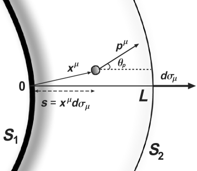
Figure 1: The picture of a gradual FO process within the finite FO layer, in x-direction, i.e. $d\sigma_{\mu}=(0,1,0,0)$. The particles are moving in different directions outwards, indicated by the angle $\theta$ . The inside boundary of the FO layer, $S_{1}$ (thick line) indicates the points where the FO starts. This is the origin of the coordinate vector, $x^{\mu}$. Within the finite thickness of the FO layer, $L$, the density of the interacting particles gradually decreases (indicated by shading) and disappears at the outside boundary, $S_{2}$ (thin line) of the FO layer.

To have a complete physical FO finished at a finite distance/time, we require: $\mathcal{P}_{esc}\rightarrow 1$, when $s\rightarrow L$. In usual cascade models the probability of collision never becomes exactly zero, and correspondingly $\mathcal{P}_{esc}$ never becomes exactly one, and the FO process lasts ad infinitum. This is due to the fact that the probability of collision is calculated based on the thermally averaged cross section, which does not vanish for thermal, e.g. Gaussian, momentum distributions. In reality the free or frozen out particles have no isotropic thermal distributions but these distributions can be anisotropic and strongly confined in the phase-space. This means that the collision probability can be exactly zero and FO may be completed in a finite space-time domain.
It seems reasonable to parameterize the escape rate, which has dimension one over length, in terms of some characteristic FO length, $\lambda^{\prime}(s,p)$,

$$W_{esc}(x^{\mu},p^{\mu},d\sigma_{\mu})\equiv\frac{1}{\lambda^{\prime}(s,p)}\Theta(p^{s})\,,$$ (4)

where the cut-off factor, $\Theta(p^{s})\equiv\Theta(p^{\mu}d\sigma_{\mu})$, forbids the FO of particles with momenta not pointing outward Bugaev_1 . This FO parameter, $\lambda^{\prime}(s,p)$, is not necessarily an average distance in space or duration in time between two subsequent collisions, like the m.f.p. The m.f.p., tends to infinity as the density decreases, while the FO just becomes faster in this limit. Actually, the FO scale behaves in the opposite way to the m.f.p. This can be seen, for example, in a simple, purely geometrical freeze out model, which takes into account the divergence of the flow in a 3D expansion Bondorf . Both this and the phase transition or clusterization effect described at the beginning of this section, lead to a finite FO layer $L$, even if the m.f.p., $\lambda_{mfp}\cong 1/n\sigma$ is still finite at the outer edge of this layer.
We consider the thickness of the layer $L$ to be the ”proper” thickness of the FO layer, because it depends only on invariant scalar matter properties like cross section, proper density, velocity divergence, phase transition or clusterization rates. These should be evaluated in the Local Rest frame (LR) of the matter, and since the layer is finite, around the middle of this layer. The proper thickness is analogous to the proper time, i.e. time measured in the rest frame of the particle, hence the proper thickness is the thickness of the FO layer measured in the rest frame attached to the freeze out front, that is, the Rest Frame of the Front (RFF). Some of the parameters like the velocity divergence and the phase transition rate describe the dynamical changes in the layer, so these can determine the properties, e.g. the thickness, of the finite layer. However, calculating $L$ from the above mentioned properties is beyond the scope of this paper, and $L$ is treated as a parameter in the following.
Let us consider the Rest Frame of the Front, where the normal vector of the front points either in time, $t$, or in space, $x$, direction, introducing the following notations. Indeed, if $d\sigma_{\mu}$ is space-like the resulting equations can be transformed into a frame where the process is stationary (here $d\sigma_{\mu}=(0,1,0,0)$ and correspondingly $s\equiv x$), while in the case of a time-like normal vector the equations can be transformed into a frame where the process is uniform and time-dependent ($d\sigma_{\mu}=(1,0,0,0)$, $s\equiv t$). For sake of transparency and simplicity we will perform calculations only for FO in a finite layer with space-like normal vector in this paper, but many intermediate results can and will be obtained in Lorentz invariant way.
Inside the FO layer particles are separated into still colliding or interacting and not-colliding or free particles. The probability not to collide with anything on the way out, should depend on the number of particles, which are in the way of a particle moving outward in the direction $\mathbf{p}/|\mathbf{p}|$ across the FO layer of thickness $L$, see Fig. 1. If we follow a particle moving outward form the beginning, ($x^{\mu}=0$), i.e. the inner surface of the FO layer, $S_{1}$, to a position $x^{\mu}$, there is still a distance

$$\frac{L-s}{\cos\theta_{\mathbf{p}}}$$

ahead of us, where $\theta_{\mathbf{p}}$ is the angle between the normal vector and $\mathbf{p}/|\mathbf{p}|$. As this remaining distance becomes smaller the probability to freeze out becomes larger, thus, we may assume that the escape rate is inversely proportional to some power, $a$, of this quantity magastalk1 ; ModifiedBTE2 .
Based on the above assumptions we write the escape rate as:

$$W_{esc}=\frac{1}{\lambda}\left(\frac{L}{L-s}\right)^{a}\left(\cos\theta_{\mathbf{p}}\right)^{a}\Theta(p^{s})\,,$$ (5)

where this newly introduced parameter, $\lambda$, is the initial, i.e. at $S_{1}$, characteristic FO length of the interacting matter, $\lambda=\lambda^{\prime}(s=0,\cos\theta_{\mathbf{p}}=1)$. The power $a$ is influencing the FO profile across the front. Indeed, calculating the escape probability, $\mathcal{P}_{esc}$, eq. (3), with the escape rate, given by eq. (5), we find

$$\mathcal{P}_{esc}=1-\left(\frac{L-s}{L}\right)^{\frac{L}{\lambda}\cos\theta_{\mathbf{p}}\Theta(p^{s})}\,,$$

for $a=1$, and

$$\mathcal{P}_{esc}=1-\exp\!\left[\frac{L}{\lambda}\,\Theta(p^{s})\frac{(\cos\theta_{\mathbf{p}})^{a}}{(a-1)}\!\left(\!1-\left(\frac{L}{L-s}\right)^{a-1}\!\right)\!\right]\,,$$

for $a\neq 1$. Thus, we see that for different $a$-values we have different FO profiles:

• $a=1$: power like FO,

• $a>1$: fast, exponential like FO,

• $a<1$: no complete FO within the finite layer, since $\mathcal{P}_{esc}$ does not tend to $1$ as $s$ approaches $L$.

In papers cikk_1 ; cikk_3 ; cikk_4 the authors were using $a=1$, and were modeling FO in an infinite layer. In order to study the effects of FO within a finite space-time domain, we would like to compare the results of our calculations with those of earlier works, therefore we shall also take $a=1$ in further calculations. It is easy to check that our escape rate, eq. (5), equals the earlier expression

$$P_{esc}=\frac{\cos\theta_{\mathbf{p}}}{\lambda}\,\Theta(p^{s})$$

in $L\rightarrow\infty$ limit. Thus, the model discussed in this paper is a generalization of the models for infinitely long FO, described in cikk_1 ; cikk_3 ; cikk_4 , and allows us to study FO in a layer of finite thickness.
The angular factor, $\cos\theta_{\mathbf{p}}$, maximized the FO probability for those particles, which propagate in the direction closest to the normal of the FO layer. For the FO in time-like directions, studied in cikk_5 , the angular factor was $1$. This factor, and correspondingly the escape rate, eq. (5), are not covariant. Furthermore, this earlier formulation does not take into account either that the escape rate of particles should be proportional to the particle velocity (the conventional non-relativistic limit of the collision rate contains the thermal average $<\sigma v>$). Let us consider the simplest situation, when the Rest Frame of the Front is the same as Rest Frame of the Gas (RFG), where the flow velocity is $u^{\mu}=(1,0,0,0)$. If freeze out propagates in space-like direction, i.e. $d\sigma_{\mu}=(0,1,0,0)$, as shown in Fig. 1, then $\cos\theta_{\mathbf{p}}=p^{x}/|\mathbf{p}|$. Therefore, a straightforward generalization of the escape rate, based on the above arguments, is

$$\cos\theta_{\mathbf{p}}\times|\mathbf{v}|\equiv\frac{p^{x}}{|\mathbf{p}|}\times\frac{|\mathbf{p}|}{p^{0}}=\bigg{(}\frac{p^{\mu}d\sigma_{\mu}}{p^{\mu}u_{\mu}}\bigg{)}\,,$$ (6)

where the r.h.s. of this equation is an invariant scalar in covariant form. Now, we assume that this simple generalization is valid for any space-like or time-like FO direction, even when RFG and RFF are different kemer ; QM05etele ; ModifiedBTE2 .
Based on the above arguments, we can write the total escape rate from eq. (5) in a Lorentz invariant form:

$$W_{esc}=\frac{1}{\lambda}\left(\!\frac{L}{L-s}\!\right)\!\!\left(\frac{p^{s}}{p^{\mu}u_{\mu}}\right)\!\Theta(p^{s})\,,$$ (7)

which now opens room for general study of FO in relativistic flow in layers of any thickness.
Former FO calculations in cikk_1 ; cikk_3 ; cikk_4 were always performed in RFF. Aiming for semianalytical results and transparent presentation, as well as in order to compare our results with former calculations, we will also study the system evolution in RFF, but now this is only our preference. In principle calculations can be performed in any reference frame. In more realistic many dimensional models, which will take into account the system expansion simultaneous with the gradual FO, it will be probably more adequate to work in RFG or in Lab frame, and our invariant escape rate, eq. (7), can be directly used as a basic FO ingredient of such models.

II.2 The Lorentz invariant escape rate

In this section let us study this new angular factor, in more detail. We will take the $p$-dependent part of the escape rate, eq. (7), and denote it as:

$$W(p)=\frac{p^{\mu}d\sigma_{\mu}}{p^{\mu}u_{\mu}}\,\Theta(p^{\mu}d\sigma_{\mu})\,.$$ (8)

In RFG, where the flow velocity of the matter is $u^{\mu}=(1,0,0,0)_{RFG}$ by definition, $W(p)$, is given as

$$W(p)=\frac{p^{\mu}d\sigma_{\mu}}{p^{0}}\,\Theta(p^{\mu}d\sigma_{\mu})\,\bigg{|}_{RFG}\,,$$ (9)

and it is smoothly changing as the direction of the normal vector changes in RFG. This will be discussed in more detail in the rest of this section.
In the following, we will take different typical points of the FO hypersurface, A, B, C, D, E, F, see Fig. 2. At these points, the normal vectors of the hypersurface, $d\sigma_{\mu}=(h,i,j,k)_{RFG}$, are given below.

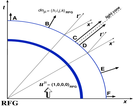
Figure 2: A simple FO hypersurface in the Rest Frame of the Gas (RFG: [t,x]), where $u^{\mu}=(1,0,0,0)_{RFG}$, including time-like and space-like parts. The normal vector of the FO front, $d\sigma_{\mu}$, is a time-like 4-vector at the time-like part and it is changing smoothly into a space-like 4-vector in the space-like part. On these two parts of the hypersurface, in the Rest Frame of the Front (RFF), $d\sigma_{\mu}$ points into the direction of the $t^{\prime}$ ($x^{\prime}$)-axis respectively. At points A,  B,  C,  D,  E,  F, we have different Rest Frame(s) of the Front, (RFF: [t’,x’]).

To calculate the normal vector for different cases shown in Fig. 2, we simply make use of the Lorentz transformation. The normal vector of the time-like part of the FO hypersurface may be defined as the local $t^{\prime}$-axis, while the normal vector of the space-like part may be defined as the local $x^{\prime}$-axis. As $d{\sigma}_{\mu}$ is normalized to unity, its components may be interpreted in terms of $\gamma_{\sigma}$ and $v_{\sigma}$, where $\gamma_{\sigma}=\frac{1}{\sqrt{1-v_{\sigma}^{2}}}$. So, we have:

• $d\sigma_{\mu}=(1,0,0,0)$, leads to $W(p)=1$,

• $d\sigma_{\mu}=\gamma_{\sigma}(1,v_{\sigma},0,0)$, leads to $W(p)=\frac{\gamma_{\sigma}(p^{0}+v_{\sigma}p^{x})}{p^{0}}$,

• $d\sigma_{\mu}=\gamma_{\epsilon}(1+\epsilon,1-\epsilon,0,0)$, where $\gamma_{\epsilon}=(4\epsilon)^{-\frac{1}{2}}$, $\epsilon\ll 1$. This leads to $W(p)=\gamma_{\epsilon}\frac{(p^{0}+p^{x})+\epsilon(p^{0}-p^{x})}{p^{0}}$,

• $d\sigma_{\mu}=\gamma_{\epsilon}(1-\epsilon,1+\epsilon,0,0)$, where $\gamma_{\epsilon}=(4\epsilon)^{-\frac{1}{2}}$,
  $\epsilon\ll 1$. This leads to $W(p)=\gamma_{\epsilon}\frac{(p^{0}+p^{x})-\epsilon(p^{0}-p^{x})}{p^{0}}\\ \times\Theta\left(\gamma_{\epsilon}(p^{0}+p^{x})-\gamma_{\epsilon}\epsilon(p^{0}-p^{x})\right)$,

• $d\sigma_{\mu}=\gamma_{\sigma}(v_{\sigma},1,0,0)$, leads to
  $\quad\,W(p)=\frac{\gamma_{\sigma}(v_{\sigma}p^{0}-p^{x})}{p^{0}}\times\Theta\Big{(}\gamma_{\sigma}(v_{\sigma}p^{0}-p^{x})\Big{)}$,

• $d\sigma_{\mu}=(0,1,0,0)$, leads to $W(p)=\frac{p^{x}}{p^{0}}\times\Theta(p^{x})$.

The resulting phase-space escape rates are shown in Fig. 3 for the six cases described above.
Similar calculations can be done in RFF, where $d\sigma_{\mu}=(1,0,0,0)$ for A, B, C and $d\sigma_{\mu}=(0,1,0,0)$ for D, E, F, leading the following values for $W(p)$:

1. $u_{\mu}=(1,0,0,0)$, leads to $W(p)=1$,

2. $u_{\mu}=\gamma_{\sigma}(1,-v_{\sigma},0,0)$, leads to
   $W(p)=\frac{p^{0}}{\gamma_{\sigma}(p^{0}-v_{\sigma}p^{x})}$,

3. $u_{\mu}=\gamma_{\epsilon}(1+\epsilon,-(1-\epsilon),0,0)$, where $\gamma_{\epsilon}=(4\epsilon)^{-\frac{1}{2}}$, $\epsilon\ll 1$. This leads to $W(p)=\frac{1}{\gamma_{\epsilon}}\frac{p^{0}}{(p^{0}-p^{x})\,+\,\epsilon(p^{0}+p^{x})}$,

4. $u_{\mu}=\gamma_{\epsilon}(1+\epsilon,-(1-\epsilon),0,0)$, where $\gamma_{\epsilon}=(4\epsilon)^{-\frac{1}{2}}$, $\epsilon\ll 1$. This leads to $W(p)=\frac{1}{\gamma_{\epsilon}}\frac{p^{0}}{(p^{0}-p^{x})\,+\,\epsilon(p^{0}+p^{x})}\\ \times\Theta(p^{x})$,

5. $u_{\mu}=\gamma_{\sigma}(1,-v_{\sigma},0,0)$, leads to
   $\quad\,W(p)=\frac{p^{x}}{\gamma_{\sigma}(p^{0}-v_{\sigma}p^{x})}\times\Theta(p^{x})$,

6. $u_{\mu}=(1,0,0,0)$, leads to $W(p)=\frac{p^{x}}{p^{0}}\times\Theta(p^{x})$.

For these cases, A, B, C, D, E, F, in RFF the resulting phase-space escape rates are shown in Fig. 4.

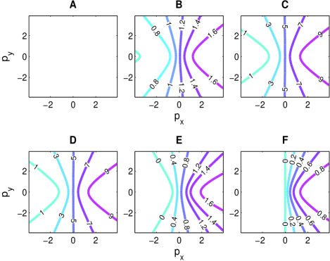
Figure 3: The contour plots of the momentum dependent part of the escape rate, $W(p)$, as in eq. (9), presented in six subplots at different points of the FO hypersurface. All plots are in RFG. For region $A$: $d{\sigma}_{\mu}=(1,0,0,0)$, and $W(p)$ is one uniformly, for $B$: $d{\sigma}_{\mu}=\gamma_{\sigma}(1,0.5,0,0)$, $C$: $d{\sigma}_{\mu}=\gamma_{\epsilon}(1.01,0.99,0,0)$, (first row), $D$: $d{\sigma}_{\mu}=\gamma_{\epsilon}(0.99,1.01,0,0)$, $E$: $d{\sigma}_{\mu}=\gamma_{\sigma}(0.5,1,0,0)$, $F$: $d{\sigma}_{\mu}=(0,1,0,0)$, (second row). The momenta are in units of particle mass, [m].

Figs. 3 and 4 show that the momentum dependence of the escape rate, uniform in point A, becomes different at different points of the FO hypersurface, but this change is continuous, when we are crossing the light cone, from point C to point D. Although in RFF, Fig. 4, it seems that there is a principal difference between space-like and time-like FO directions, due to the cut-off $\Theta(p^{\mu}d\sigma_{\mu})$ function, but this is only the consequence of the chosen reference frame, i.e. RFF is defined in a way to stress the difference between these two cases, since going from C to D, the normal vector has a jump, i.e. $d\sigma_{\mu}=(1,0,0,0)$ goes over to $d\sigma_{\mu}=(0,1,0,0)$. Nevertheless, $W(p)$ is a continuous function as we change $d\sigma_{\mu}$, and in other frames, for example in RFG, Fig. 3, we can see this clearly.

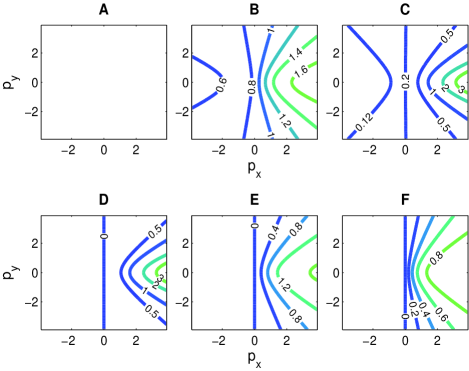
Figure 4: The contour plots of the momentum dependent part of the escape rate, $W(p)$, in RFF. For region $A$: $u_{\mu}=(1,0,0,0)$, and $W(p)$ is one uniformly, for $B$: $u_{\mu}=\gamma_{\sigma}(1,-0.5,0,0)$, $C$: $u_{\mu}=\gamma_{\epsilon}(1.01,-0.99,0,0)$, (first row), $D$: $u_{\mu}=\gamma_{\epsilon}(1.01,-0.99,0,0)$, $E$: $u_{\mu}=\gamma_{\sigma}(1,-0.5,0,0)$, $F$: $u_{\mu}=(1,0,0,0)$, (second row). In cases D, E, F the escape rate vanishes for momenta with $p_{x}<0$. The momenta are in units of particle mass, [m].

II.3 The updated simple kinetic model

Now, using the new invariant escape rate, eq. (7), we can generalize the simple model presented in cikk_1 ; cikk_3 ; cikk_4 , i.e. eqs. (II.1), for a finite space-time FO layer:

$$\partial_{s}f_{i}\,ds = -\left(\!\frac{L}{L-s}\!\right)\!\left(\frac{p^{s}}{p^{\mu}u_{\mu}}\right)\!\Theta(p^{s})f_{i}\,\frac{ds}{\lambda}\,,$$

$$\partial_{s}f_{f}\,ds = \left(\!\frac{L}{L-s}\!\right)\!\left(\frac{p^{s}}{p^{\mu}u_{\mu}}\right)\!\Theta(p^{s})f_{i}\,\frac{ds}{\lambda}\,,$$ (10)

Solving the first equation we find for the interacting component:

$$f_{i}(s,p) = f_{J}(p)\left(\!\frac{L-s}{L}\right)^{\frac{L}{\lambda}\left(\frac{p^{s}}{p^{\mu}u_{\mu}}\right)\Theta(p^{s})}\,$$ (11)

$$\buildrel s\rightarrow L\over{\longrightarrow} f_{J}(p)\,\Theta(-p^{s})\,.$$

Now, inserting this result into the second differential equation, from eqs. (II.3), we obtain the FO solution, which describes the momentum distribution of the frozen out particles:

$$f_{f}(s,p) = f_{J}(p)\,\left[1-\left(\!\frac{L-s}{L}\!\right)^{\frac{L}{\lambda}\left(\frac{p^{s}}{p^{\mu}u_{\mu}}\right)\!\Theta(p^{s})}\right]\,$$ (12)

$$\buildrel s\rightarrow L\over{\longrightarrow} f_{J}(p)\,\Theta(p^{s})\,.$$

As $s$ tends to $L$, i.e. to the outer boundary of the FO layer, this distribution, depending on the direction of the normal vector (space-like) or time-like will tend to the (cut) Jüttner distribution, $f_{J}(p)$. This means that (part of) the original Jüttner distribution survives even when we reach the outer boundary of the FO surface. To remedy this highly unrealistic result, in cikk_1 ; cikk_3 ; cikk_4 ; cikk_5 , rethermalization in the interacting component was taken into account via the relaxation time approximation, i.e. we insert into the equation for the interacting component a new term, which describes that the interacting component approaches some equilibrated (Jüttner) distribution, $f_{eq}(s)$, with a relaxation length, $\lambda_{0}$:

$$\partial_{s}f_{i}ds = -\left(\!\frac{L}{L-s}\!\right)\!\left(\frac{p^{s}}{p^{\mu}u_{\mu}}\right)\!\Theta(p^{s})f_{i}\,\frac{ds}{\lambda}$$

$$+ \quad\left[f_{eq}(s)-f_{i}\right]\frac{ds}{\lambda_{0}}\,,$$

$$\partial_{s}f_{f}ds = \left(\!\frac{L}{L-s}\!\right)\!\left(\frac{p^{s}}{p^{\mu}u_{\mu}}\right)\!\Theta(p^{s})f_{i}\,\frac{ds}{\lambda}\,.$$ (14)

Let us concentrate on the equation for the interacting component. Here the first term from eq. (II.3), related to FO, moves the distribution out of the equilibrium, and decreases the energy-momentum density and baryon density of the interacting particles. The second term from eq. (II.3), changes the distribution in the direction of the thermalization, while it does not effect the conserved quantities. The relative strength of the FO and rethermalization processes is determined by the two characteristic lengths, $\lambda$ and $\lambda_{0}$.
In general the evolution of the interacting component can be solved numerically or semianalytically, at every step of the integration. Then, the change of conserved quantities due to FO should be evaluated using the actual distribution, $f_{i}(s,p)$ at the corresponding point $s$. For the purpose of this work, namely for the qualitative study of the FO features, it is enough to use an approximate solution, similarly as it was done in cikk_3 ; cikk_4 ; cikk_5 . This would also allow us to make a direct comparison with results of these older calculations. Thus, the evaluation of the change of the conserved quantities is done analytically, i.e. $f_{i}(s,p)$ is approximated with an equilibrium distribution function $f_{eq}(s)$ with parameters, $T(s),\,n(s),\,u^{\mu}(s)$.
This approximation is based on the fact that in most physical situations the overall number of particle collisions vastly exceeds the number of those collisions, after which a particle leaves the system or freezes out. This allows us to take that rethermalization happens faster than the freeze out, i.e. that $\lambda_{0}<\lambda$ or $\lambda_{0}\ll\lambda$. Of course, this argument is true only at the beginning of the FO process, when the density of the interacting particles is still large. When $s$ is close to $L$, i.e. near the outer hypersurface, the first term in eq. (II.3) becomes more important than the rethermalization term because of its denominator, but as we shall see in the results section, particles freeze out exponentially fast and for large $s$, when say $99\%$ of the matter is frozen out, the error we introduce with our approximate solution can not really affect the physical situation.

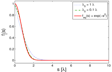
Figure 5: Numerical solutions of eq. (II.3) for different $\lambda_{0}$’s. This solution was obtained using, $f_{eq}=e^{-s^{2}}$, test function, for $L=10\lambda$. The results show that $f_{i}(s)$ approaches $f_{eq}(s)$ when $\lambda_{0}\ll\lambda$.

For illustration, let us take a test function, $f_{eq}(s)=e^{-s^{2}}$, (we ignore $p$ dependence for the moment), which is a smoothly and fastly decreasing function. In Fig. 5 we show the numerical solutions for the interacting component for $\lambda_{0}=\lambda$ and $\lambda_{0}=0.1\lambda$. The results show that for the latter case we can safely take for the $f_{i}$ the approximate solution cikk_3 ; cikk_4 ; cikk_5 :

$$f_{i}(s)=f_{eq}(s)\,.$$ (15)

II.4 Conservation Laws

The goal of the freeze out calculations is to find the final post FO momentum distribution, and then the corresponding quantities defined through it, starting from the initial pre FO distribution. On the pre FO side we can have equilibrated matter or gas. Its local rest frame defines the RFG, see Fig. 6. We can also define the reference frame, which is attached to the freeze out front, namely the RFF, see Fig. 7. These choices are usually advantageous, but other choices are also possible.

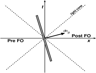
Figure 6: The orientation of the freeze out front in RFG is given as, $d\sigma_{\mu}=\gamma_{\sigma}(v_{\sigma},1,0,0)_{RFG}$.

Furthermore, the conservation laws and the nondecreasing entropy condition must be satisfied cikk_1 :

$$\left[N^{\mu}d\sigma_{\mu}\right]=0\,,\quad\left[T^{\mu\nu}d\sigma_{\mu}\right]=0\,,\quad\left[S^{\mu}d\sigma_{\mu}\right]\geq 0\,,$$ (16)

where $\left[A\right]=A-A_{0}$. The pre FO side baryon and entropy currents and the energy-momentum tensor are denoted by $N^{\mu}_{0},S^{\mu}_{0},T^{\mu\nu}_{0}$, while the post FO quantities are denoted by $N^{\mu},S^{\mu},T^{\mu\nu}$.
The change of conserved quantities caused by the particle transfer from the interacting matter to the free matter can be obtained in the following way. For the conserved particle 4-current we have

$$dN^{\mu}=dN^{\mu}_{i}+dN^{\mu}_{f}=0\ \Rightarrow\ dN^{\mu}_{i}=-dN^{\mu}_{f}\,.$$ (17)

Then, using the kinetic definition of the particle current, together with eqs. (14, 15), we obtain

$$dN^{\mu}_{i}(s)\! = -\ ds\!\int\!\frac{d^{3}p}{p^{0}}p^{\mu}\left[\partial_{s}f_{f}\right]$$

$$= \!-\frac{ds}{\lambda}\!\left(\!\frac{L}{L-s}\!\right)\!\!\!\int\!\frac{d^{3}p}{p^{0}}p^{\mu}\!\left[\frac{p^{s}}{p_{\,\rho}u^{\rho}_{i}}\Theta(p^{s})\right]\!f_{eq}(s)\,.$$

Similarly the change in the energy-momentum is

$$dT^{\mu\nu}_{i}(s)=-\frac{ds}{\lambda}\!\left(\!\frac{L}{L-s}\!\right)\!\!\!\int\!\frac{d^{3}p}{p^{0}}\,p^{\mu}p^{\nu}\left[\frac{p^{s}}{p_{\,\rho}u^{\rho}_{i}}\,\Theta(p^{s})\right]\!f_{eq}(s)\,.$$ (19)

The parameters of the equilibrium (Jüttner) distribution, $f_{eq}(s)$, have to be recalculated after each step, $ds$, from the conservation laws as in cikk_3 ; cikk_4 ; cikk_5 .

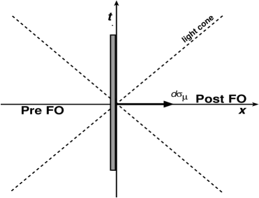
Figure 7: The orientation of the freeze out front in RFF, i.e. in its own rest frame, is $d\sigma_{\mu}=(0,1,0,0)_{RFF}$. In this frame the gas has nonvanishing velocity in general.

The change of flow velocity, $du^{\mu}_{i}(s)$, can be calculated using Eckart’s or Landau’s definition of the flow, i.e. from $dN^{\mu}_{i}(s)$ or $dT^{\mu\nu}_{i}(s)$ correspondingly. Then the change of conserved particle density is given by

$$dn_{i}(s)=u^{\mu}_{i}(s)\,dN^{\mu}_{i}(s)\,,$$ (20)

and for the change of energy density we have

$$de_{i}(s)=u_{\mu,i}(s)\,dT^{\mu\nu}_{i}(s)\,u_{\nu,i}(s)\,.$$ (21)

The change of the temperature of interacting component can be found from this last equation, eq. (21), and from the Equation of State (EoS). This closes our system of equations.
If we fix the FO direction to the $x$-direction, then eqs. (II.4,19) can be rewritten as:

$$dN^{\mu}_{i}(x) = -\frac{dx}{\lambda}\!\left(\!\frac{L}{L-x}\!\right)\!\int\frac{d^{3}p}{p^{0}}\,p^{\mu}\,$$

$$\times \left[\frac{p\cos\theta_{\mathbf{p}}}{\gamma(p^{0}-jup\,\cos{\theta}_{\mathbf{p}})}\Theta(\cos\theta_{\mathbf{p}})\right]\!f_{eq}(x,p)\,,$$

and

$$dT^{\mu\nu}_{i}(x) = -\frac{dx}{\lambda}\!\left(\!\frac{L}{L-x}\!\right)\!\int\frac{d^{3}p}{p^{0}}\,p^{\mu}p^{\nu}\,$$

$$\times \left[\frac{p\cos\theta_{\mathbf{p}}}{\gamma(p^{0}-jup\,\cos{\theta}_{\mathbf{p}})}\Theta(\cos\theta_{\mathbf{p}})\right]\!f_{eq}(x,p)\,,$$

where, the four momentum of particles is $p^{\mu}=(p^{0},\mathbf{p})$, $p=|\mathbf{p}|$, $p^{x}=p\cos\theta_{\mathbf{p}}$, the flow velocity of the interacting matter is $u^{\mu}_{i}=\gamma(1,v,0,0)$, $\gamma=\frac{1}{\sqrt{1-v^{2}}}$, $u=|v|$ and $j=sign(v)$ .

II.5 Changes of the conserved current and energy-momentum tensor

In this section we show new analytical results for the changes of the conserved particle current and energy-momentum tensor. The formulae are analogous to those from ref. cikk_1 ; cikk_3 , but now they are calculated with the Lorentz invariant angular factor from eq. (7). We show results for both massive and massless particles.

$$dN^{0}_{i}(x) = -\frac{dx}{\lambda}\bigg{(}\frac{L}{L-x}\bigg{)}\frac{n}{4u^{2}\gamma^{2}}\Bigg{\{}\gamma G_{1}^{-}(m)+\frac{b^{3}\Gamma(0,b)}{3\gamma^{2}}-2\gamma bu\Big{[}(1+j)K_{1}(a)-\mathcal{K}_{1}(a,b)\Big{]}$$

$$- ub^{2}\Big{[}(1+j)K_{0}(a)-\mathcal{K}_{0}(a,b)\Big{]}+\bigg{[}u^{2}\gamma^{2}(1+b)(u^{2}-3)-\frac{A(b)}{3\gamma^{2}}\bigg{]}e^{-b}\Bigg{\}}$$

$$\buildrel m=0\over{\longrightarrow} -\frac{dx}{\lambda}\bigg{(}\frac{L}{L-x}\bigg{)}\frac{n}{4}\Bigg{[}\frac{(3-v)(1+v)^{3}}{3}\gamma^{2}\Bigg{]}\,,$$

$$dN^{x}_{i}(x) = \frac{dN^{0}_{i}(x)}{ju}\,-\,\frac{dx}{\lambda}\,\bigg{(}\!\frac{L}{L-x}\bigg{)}\,\frac{n}{4u^{2}\gamma^{2}}\Bigg{\{}-2j\gamma bu^{2}\Big{[}(1+j)K_{1}(a)-\mathcal{K}_{1}(a,b)\Big{]}$$ (24)

$$- \,\,\,jb^{2}u^{2}\Big{[}(1+j)K_{0}(a,b)-\mathcal{K}_{0}(a,b)\Big{]}-ju\gamma^{2}(1+u^{2})(1+b)e^{-b}\Bigg{\}}$$

$$\buildrel m=0\over{\longrightarrow} -\frac{dx}{\lambda}\,\bigg{(}\!\frac{L}{L-x}\bigg{)}\frac{n}{4}\Bigg{[}\frac{2(1+v)^{3}}{3}\,\gamma^{2}\Bigg{]}\,,$$

$$dT^{00}_{i}(x) = -\frac{dx}{\lambda}\,\bigg{(}\!\frac{L}{L-x}\bigg{)}\,\frac{nT}{4u^{2}\gamma^{2}}\Bigg{\{}\frac{b^{4}\Gamma(0,b)}{4\gamma^{3}}-\gamma G_{2}^{-}(m)-u\gamma b^{2}(u^{2}+3)\Big{[}(1+j)K_{2}(a)-\mathcal{K}_{2}(a,b)\Big{]}$$

$$- ub^{3}\Big{[}(1+j)K_{1}(a)-\mathcal{K}_{1}(a,b)\Big{]}+\gamma^{3}\bigg{[}-A(b)(3u^{2}+1)+\frac{B(b)}{2\gamma^{6}}-\frac{b^{2}(3+b)}{3\gamma^{6}}$$

$$- \frac{b^{2}u^{2}(1+b)}{\gamma^{6}}+\frac{2}{3}b^{3}u^{4}(u^{2}-3)+a^{2}\bigg{]}e^{-b}\,\Bigg{\}}$$

$$\buildrel m=0\over{\longrightarrow} -\frac{dx}{\lambda}\,\bigg{(}\!\frac{L}{L-x}\bigg{)}\frac{nT}{4}\Bigg{[}\frac{(1+v)^{4}}{2}(6-4v+v^{2})\gamma^{3}\Bigg{]}\,,$$

$$dT^{0x}_{i}(x) = \frac{dT^{00}_{i}(x)}{ju}\,-\,\frac{dx}{\lambda}\,\bigg{(}\!\frac{L}{L-x}\bigg{)}\,\frac{nT}{4u^{2}\gamma^{2}}\Bigg{\{}-j\gamma b^{2}(3u^{2}+1)\Big{[}(1+j)K_{2}(a)-\mathcal{K}_{2}(a,b)\Big{]}$$

$$- jb(b^{2}u^{2}-2)\Big{[}(1+j)K_{1}(a)-\mathcal{K}_{1}(a,b)\Big{]}+jab\Big{[}(1+j)K_{0}(a)-\mathcal{K}_{0}(a,b)\Big{]}$$

$$- ju\gamma\Big{[}\gamma^{2}A(b)(u^{2}+3)+(1+b)(u^{2}-3)+\frac{4b^{3}}{3}u^{2}\gamma^{2}-b^{2}\Big{]}e^{-b}\Bigg{\}}$$

$$\buildrel m=0\over{\longrightarrow} -\frac{dx}{\lambda}\,\bigg{(}\!\frac{L}{L-x}\bigg{)}\frac{nT}{4}\Bigg{[}\frac{(1+v)^{4}}{2}(4-v)\gamma^{3}\Bigg{]}\,,$$

$$dT^{xx}_{i}(x) = \frac{dT^{0x}(x)}{ju}\,-\,2\frac{T}{\gamma ju}\Bigg{[}dN^{x}_{i}\,-\,\frac{dN^{0}_{i}(x)}{ju}\Bigg{]}$$

$$- \frac{dx}{\lambda}\,\bigg{(}\!\frac{L}{L-x}\bigg{)}\,\frac{nT}{4u^{2}\gamma^{2}}\Bigg{\{}-\gamma ub^{2}(3+u^{2})\Big{[}(1+j)K_{2}(a)-\mathcal{K}_{2}(a,b)\Big{]}$$

$$+ \gamma^{3}\Big{[}A(b)(3u^{2}+1)+\frac{2}{3}b^{3}u^{4}(u^{2}-3)+a^{2}\Big{]}e^{-b}\,\Bigg{\}}$$

$$\buildrel m=0\over{\longrightarrow} -\frac{dx}{\lambda}\,\bigg{(}\!\frac{L}{L-x}\bigg{)}\frac{nT}{4}\Bigg{[}\frac{3(1+v)^{4}}{2}\gamma^{3}\Bigg{]}\,,$$

$$dT^{yy}_{i}(x) = -\frac{dT^{xx}(x)}{2}\,-\,\frac{dx}{\lambda}\,\bigg{(}\!\frac{L}{L-x}\bigg{)}\,\frac{nT}{8u^{2}\gamma^{2}}\Bigg{\{}-\gamma ub^{2}(3+u^{2})\Big{[}(1+j)K_{2}(a)-\mathcal{K}_{2}(a,b)\Big{]}$$

$$+ \gamma^{3}\Big{[}A(b)(3u^{2}+1)-\frac{3B(b)}{2\gamma^{6}}+\frac{(b^{2}+1)(1+b)}{2\gamma^{6}}+\frac{2}{3}b^{3}u^{4}(u^{2}-3)+a^{2}\Big{]}e^{-b}-\frac{b^{4}\Gamma(0,b)}{4\gamma^{3}}+\gamma H_{2}^{-}(m)\Bigg{\}}$$

$$\buildrel m=0\over{\longrightarrow} -\frac{dx}{\lambda}\,\bigg{(}\!\frac{L}{L-x}\bigg{)}\frac{nT}{8}\Bigg{[}\frac{\gamma(1+v)^{3}}{4v^{2}}(-4+12v-9v^{2}+3v^{3})\Bigg{]}\,,$$

and

$$dT^{zz}_{i}(x)=dT^{yy}_{i}(x)\,,$$ (25)

where, $a=\frac{m}{T}$, $b=a\gamma$, $A(b)=(2+2b+b^{2})e^{-b}$, $B(b)=\frac{1}{6}(6+6b+3b^{2}+b^{3})e^{-b}$ and $n=4\pi T^{3}a^{2}K_{2}(a)\,g\,\frac{e^{\mu/T}}{(2\pi\hbar)^{3}}$ is the particle density, $g$ is the degeneracy factor while, $G^{-}(m)$, $H^{-}(m)$, $\mathcal{K}(a,b)$, $K(a)$, $\Gamma(0,b)$ are defined in Appendix A. Note that the $x$-dependent factor $L/(L-x)$ is just a multiplier in these calculations, and tends to unity if we are dealing with an infinitely long FO, as in cikk_1 ; cikk_3 ; cikk_4 .

III Results and Discussion

In this section we calculate the post FO distributions and compare the results to former calculations presented in cikk_1 ; cikk_3 ; cikk_4 . The effect of two main differences due to the new Lorentz invariant escape rate, eq. (7), is to be checked:

1. the infinite, $(\infty)$, FO layer or finite, $(L)$, FO layer,

2. the simple angular escape rate, $P$, or the covariant escape rate, $W$.

We performed calculations for a baryonfree massless gas, where we have used a simple EoS, $e=\sigma_{SB}T^{4}$, where $\sigma_{SB}=\frac{\pi^{2}}{10}$. The change of temperature is calculated based on this EoS and eq. (21). There are no conserved charges in our system, consequently we use Landau’s definition of the flow velocity cikk_3 :

$$du^{\mu}_{i,Landau}(x)=\frac{\Delta^{\mu\nu}_{i}(x)\ \ dT_{i,\nu\sigma}(x)\ \ u^{\sigma}_{i}(x)}{e_{i}(x)+P_{i}(x)}\,,$$ (26)

where $\Delta^{\mu\nu}_{i}(x)=g^{\mu\nu}-u_{i}^{\mu}(x)\,u_{i}^{\nu}(x)\,$ is a projector to the plane orthogonal to $u^{\mu}_{i}(x)$, while $e_{i}(x)$ and $P_{i}(x)$ are the local energy density and pressure of the interacting component, i.e. $T^{\mu\nu}_{i}(x)=(e_{i}(x)+P_{i}(x))u_{i}^{\mu}(x)u_{i}^{\nu}(x)-P_{i}(x)g^{\mu\nu}$. A detailed treatment of Eckart’s flow velocity can be found in cikk_1 ; cikk_3 .
For such a system we finally obtain the following set of differential equations:

$$d\ln T = \frac{\gamma^{2}}{4\sigma_{SB}T^{4}}\bigg{[}dT^{00}_{i}-2vdT^{0x}_{i}+v^{2}dT^{xx}_{i}\bigg{]}\,,$$ (27)

$$dv = \frac{3}{4\sigma_{SB}T^{4}}\bigg{[}-vdT^{00}_{i}+(1+v^{2})dT^{0x}_{i}-vdT^{xx}_{i}\bigg{]}\,.$$

We will present the results for four different cases:

• We use the simple, but relativistically not invariant angular factor, $\cos\theta_{\mathbf{p}}$, in the escape rate,

  $$P_{\infty}=\frac{\cos\theta_{\mathbf{p}}}{\lambda}\Theta(p\cos\theta_{\mathbf{p}})\,.$$

  The system is characterized by an infinite FO length (up to $x_{max}=300\lambda$ in calculations). The results are shown in Figs. (8, 10, 12). This is the same model as in cikk_1 ; cikk_3 ; cikk_4 .

• Next, we are using the simple angular factor, but in this case inside a finite FO layer, $L=10\lambda$,

  $$P_{L}=\left(\frac{L}{L-x}\right)\frac{\cos\theta_{\mathbf{p}}}{\lambda}\Theta(p\cos\theta_{\mathbf{p}})\,.$$

  The results are shown in Figs. (9, 11, 14).

• Then, we are dealing with the new Lorentz invariant angular factor in the escape rate and with an infinite FO length, $x_{max}=300\lambda$,

  $$W_{\infty}=\frac{1}{\lambda}\left(\frac{p\cos\theta_{\mathbf{p}}}{p^{\mu}u_{\mu}}\right)\Theta(p\cos\theta_{\mathbf{p}})\,.$$

  The results are shown in Figs. (8, 10, 12, 13).

• Finally we present the primary results of this paper, using both our new improvements, i.e. the covariant escape rate of eq. (7),

  $$W_{L}=\frac{1}{\lambda}\left(\frac{L}{L-x}\right)\left(\frac{p\cos\theta_{\mathbf{p}}}{p^{\mu}u_{\mu}}\right)\Theta(p\cos\theta_{\mathbf{p}})\,.$$

  The results are shown in Figs. (9, 11, 14, 15).

In the case of FO in the infinite layer the factor, $L/(L-x)$, was replaced by $1$. We presented the situation at a distance of $x_{max}=300\lambda$, where the amount of still interacting particles is negligible.
For the particular cases when we are dealing with an infinite FO, i.e. $P_{\infty}$ and $W_{\infty}$, or with finite layer FO, i.e. $P_{L}$ and $W_{L}$, the results are plotted together. Thus, in one figure the focus is on the consequences caused by the different angular factors.
Thin lines always denote the cases with simple relativistically not invariant angular factor, these correspond to $P_{\infty}$ and $P_{L}$. Thick lines always correspond to cases with covariant angular factor, $W_{\infty}$ and $W_{L}$.
All the figures are presented in the RFF.

III.1 The evolution of temperature of the interacting component

The first set of figures, Figs. 8, 9, shows the evolution of temperature of the interacting component, in fact the gradual cooling of the interacting matter, for the different cases, $P_{\infty},P_{L},W_{\infty}$ and $W_{L}$.
First, on all figures matter with larger (positive) flow velocity, $v_{0}$, cools faster. This is caused by the momentum dependence of the escape rate, which basically tells that faster particle in the FO direction, will freeze out faster. Thus, the remaining interacting component cools down, since the most energetic particles freeze out more often than the slow ones. Of course, for larger initial flow velocity, $v_{0}$, in the FO direction, there are more particles moving in the FO direction with higher momenta in average, than for a smaller flow velocity.
Now, comparing Fig. 8 with Fig. 9, we can see the difference between finite and infinite FO dynamics. In a finite layer the cooling of interacting matter goes increasingly faster as FO proceeds, while for FO in infinite layer the cooling gradually slows down as $x$ increases. The reason is the factor, $L/(L-x)$, which speeds up FO as $L-x$ decreases, and forces it to be completed within $L$.

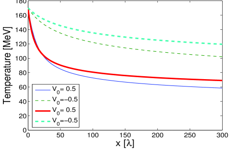
Figure 8: The temperature of the interacting component in RFF for a baryonfree massless gas, calculated with the two escape rates: $P_{\infty}$ (thin lines) and $W_{\infty}$ (thick lines), for an infinitely long FO, $(x_{max}=300\lambda)$. The initial temperature is $T_{0}=170$ MeV, $v_{0}$ is the initial velocity in RFF.

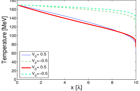
Figure 9: The temperature of the interacting component in RFF, calculated with the two escape rates: $P_{L}$ (thin lines) and $W_{L}$ (thick lines), for a finite, $(L=10\lambda)$, FO layer. The initial temperature is $T_{0}=170\,$ MeV, $v_{0}$ is the initial velocity in RFF.

The difference between $P$ and $W$ escape rates comes from the denominator, which is $p^{0}$ in case of $P$ and $p^{\mu}u_{\mu}$ in case of $W$. This difference leads to a stronger cooling for the escape rate $P$ which is bigger than $W$, if $v_{0}\neq 0$. This can be seen well at later stages of infinitely long FO, Fig. 8, particularly for the positive initial flow velocity. In all other cases the difference between old and new angular factors is insignificant, what supports our ”naive” generalization of the angular factor.

III.2 The evolution of common flow velocity of the interacting component

The second set of figures, Figs. 10, 11, shows the evolution of the flow velocity of the interacting component.
In both cases the flow velocity of the interacting component tends to $-1$, because the FO points to the positive direction and particles with positive momenta freeze out. Thus, the mean momentum of the rest must become negative.

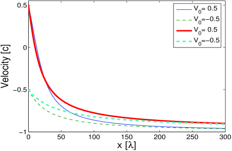
Figure 10: The flow velocity of the interacting component in RFF for a baryonfree massless gas, calculated with the two escape rates: $P_{\infty}$ (thin lines) and $W_{\infty}$ (thick lines), for an infinitely long FO, $(x_{max}=300\lambda)$. The initial temperature is $T_{0}=170$ MeV, $v_{0}$ is the initial velocity in RFF.

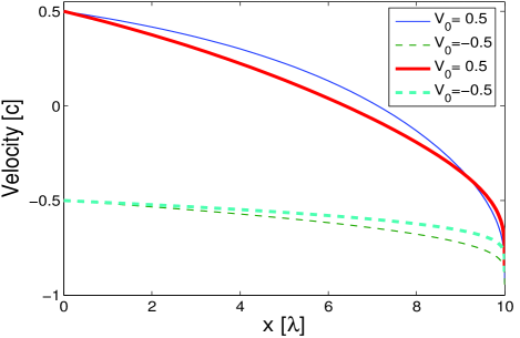
Figure 11: The flow velocity of the interacting component in RFF, calculated with the two escape rates: $P_{L}$ (thin lines) and $W_{L}$ (thick lines), for a finite, $(L=10\lambda)$, FO layer. The initial temperature is $T_{0}=170$ MeV, $v_{0}$ is the initial velocity in RFF.

Comparing Fig. 10 with Fig. 11, we can see again that in a finite layer the flow velocity decreases faster and faster as FO proceeds, while for FO in infinite layer the velocity change gradually slows down as $x$ increases. The reason is the $L/(L-x)$ factor, as discussed above.
The difference between the evolution of the flow velocity, due to the different angular factors, is again not significant, supporting its generalization.

III.3 The evolution of the transverse momentum and contour plots of the post FO distribution

The next set of figures, Figs. 12, 13, shows the evolution of the transverse momentum distribution, while Figs. 14, 15, present the contour plots of the post FO momentum distribution, for $W_{\infty}$ and $W_{L}$. We have presented a one-dimensional model here, but we assume that it is applicable for the direction transverse to the beam in heavy ion experiments. The presented plots should be qualitatively compared to the transverse momentum distributions of measured pions.

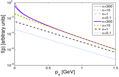
Figure 12: The local transverse momentum (here $p_{x}$) distribution for a baryonfree massless gas at $(p_{y}=0)$, calculated with the two escape rates: $P_{\infty}$ (thin lines) and $W_{\infty}$ (thick lines), for an infinitely long FO, $(x_{max}=300\lambda)$. The initial parameters are $v_{0}=0$ and $T_{0}=170\,$MeV. The transverse momentum spectrum is obviously curved due to the freeze out process. The slope of the transverse momentum distribution increases as we are approaching infinity.

What we see is that all the final post FO momentum distributions are essentially the same. This is very important outcome from our analysis, which we will discuss below. Also, one can see that resulting post FO distributions are non-thermal distributions, as it has been shown already in cikk_1 ; cikk_3 ; cikk_4 , they strongly deviate from exponential form in the low momentum region. The increase in the final FO spectra over the thermal distribution for low momenta is connected to the fact that at late stages of the FO process, the interacting component is cold and its flow velocity is negative. So, it contributes only to the low momentum region of the post FO spectra.

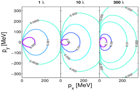
Figure 13: The post FO distribution, $f_{f}(x,\mathbf{p})$, in RFF. The calculations were done with the Lorentz invariant escape rate, $W_{\infty}$, for an infinitely long FO, $(x_{max}=300\lambda)$. The subplots correspond to $x=1\lambda,\ 10\lambda,\ 300\lambda$ respectively. The initial parameters are $v_{0}=0$ and $T_{0}=170\,$MeV. Contour lines are given at values represented on the figure. The maximum is increasing with $x$ as indicated in Fig. 12. The distribution is asymmetric and elongated in the FO direction. This may lead to a large-$p_{t}$ enhancement, compared to the usual Jüttner assumption used in many earlier calculations as a post freeze out distribution. Note that $f_{f}(x,\mathbf{p})$ does not tend to the cut Jüttner distribution even at very large $x$.

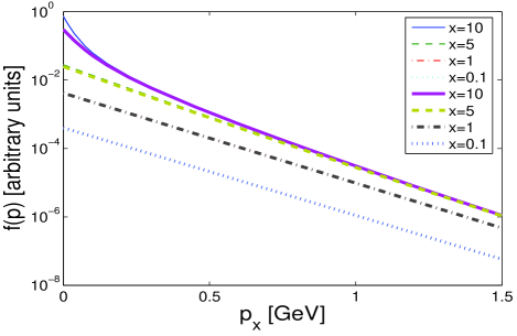
Figure 14: The local transverse momentum (here $p_{x}$) distribution for a baryonfree massless gas at $(p_{y}=0)$, calculated with the two escape rates: $P_{L}$ (thin lines) and $W_{L}$ (thick lines) for a finite, $(L=10\lambda)$, FO layer. The initial parameters are $v_{0}=0$ and $T_{0}=170\,$MeV.

These results were obtained in a stationary one-dimensional model with a single flow velocity. In reality different space-time sections of the overall FO layer are moving with respect to each other with considerable velocities, i.e. $v\approx 0.2-0.7$. Therefore, the superposition of these parts of the FO layer wash out the very sharp peaks at small momenta, while the curvature at higher momenta, although it is smaller, may persist even after superposition. There are several effects mentioned in the literature, which can cause such a curvature. The effects discussed in this section, arising from kinetic description, may contribute to the curvature of the spectra, but we need a more realistic full scale, nonstationary 3-dimensional model to estimate the expected shape of the $p_{t}$ spectra in measurements. Consequently, both the contributions of space-like and time-like sections of the FO layer have to contribute.

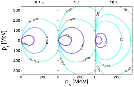
Figure 15: The post FO distribution, $f_{f}(x,\mathbf{p})$, in RFF. The calculation was made using the covariant escape rate, $W_{L}$ for a finite, $(L=10\lambda)$, FO layer. The subplots correspond to $x=0.1\lambda,\ 1\lambda,\ 10\lambda$ respectively. The initial parameters are $v_{0}=0$ and $T_{0}=170\,$MeV. Contour lines are given at values represented on the figure.

III.4 Freeze out in layers of different thickness

In this section we show the results of calculations performed with $W_{L}$ escape rate, for different finite FO layer thicknesses. Some results of such an analysis have also been presented in QM05 .
In Figs. 16, 17, we present the evolution of the temperature and flow velocity of the interacting component for $L=2\lambda,\ 5\lambda,\ 10\lambda,\ 15\lambda$. We plot the resulting curves as function of $x/L$, what allows us to present them all in one figure. We clearly see, and this agrees also with our previous comparison to infinitely long FO, that by introducing and varying the thickness of the FO layer, we are strongly affecting the evolution of the interacting component.
We can also study how fast the energy density of the interacting component is decreasing, see Fig. 18. Since there is no expansion in our simple model, the evolution of the energy density is equivalent to the evolution of the total energy of the remaining interacting matter. We can see that the decrease of the energy density of the interacting component is exponentially fast, what justifies our way of getting approximate an solution for the interacting component, see section II.3.

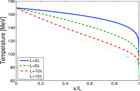
Figure 16: The evolution of the temperature of the interacting component in RFF, for a baryonfree massless gas, calculated with the $W_{L}$ escape rate for different FO layer thicknesses $L=2\lambda,\ 5\lambda,\ 10\lambda,\ 15\lambda$. The initial parameters are $v_{0}=0.5$ and $T_{0}=170\,$MeV.

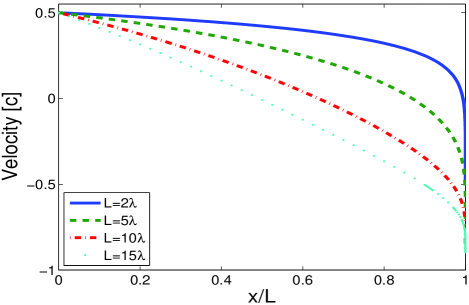
Figure 17: The evolution of the flow velocity of the interacting component in RFF, for a baryonfree massless gas, calculated with the $W_{L}$ escape rate for different FO layer thicknesses $L=2\lambda,\ 5\lambda,\ 10\lambda,\ 15\lambda$. The initial parameters are $v_{0}=0.5$ and $T_{0}=170\,$MeV.

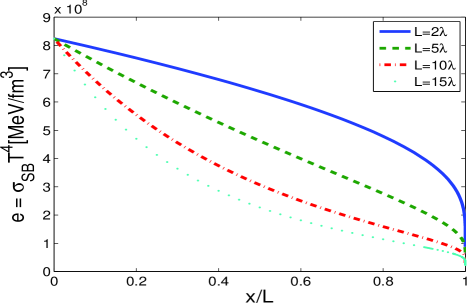
Figure 18: The evolution of the energy density of the interacting component in RFF, for a baryonfree massless gas, $\sigma_{SB}=\pi^{2}/10$, calculated with the $W_{L}$ escape rate for different FO layer thicknesses $L=2\lambda,\ 5\lambda,\ 10\lambda,\ 15\lambda$. The initial parameters are $v_{0}=0.5$ and $T_{0}=170\,$MeV.

Figure 19 shows the final post FO transverse momentum distribution for different $L$. Despite the differences in the evolution of the interacting component, all the final post FO distributions look the same and are practically indistinguishable. The difference between the result for a FO layer as thin as $L=2\lambda$ and that for $L\rightarrow\infty$ limit shows up only in the low momentum region, and it is not significant enough to allow us to resolve layers of different thicknesses from experimental spectra. Thus, the thickness of the FO layer does not affect, as we have seen already in the previous section, the final post FO distribution, which is in fact the measured quantity!

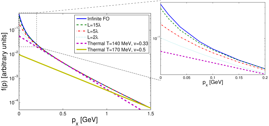
Figure 19: Final post FO transverse momentum (here $p_{x}$) distributions for the FO layers of different thicknesses. Calculations were done for baryonfree massless gas with escape rate $W_{L}$ for $L=2\lambda,\ 5\lambda,\ 15\lambda$ and with $W_{\infty}$ (thick line). The initial conditions are the same as in Figs. 16, 17: $T_{0}=170\ MeV$, $v_{0}=0.5$. Distributions for the different FO layer thicknesses are very similar, with some difference in the low momenta region, which is shown in more detail in the ”zoom in” subplot. The two thick lines correspond to some effective thermal distributions, with the corresponding parameters displayed in the plot legend. These are shown to illustrate the difference between obtained post FO distributions and thermal distributions.

IV Conclusions and outlook

In this paper we presented a simplified, but still non-trivial, Lorentz invariant freeze out model, which allows us to obtain analytical results in the case of a massless baryonfree gas. In addition the model realizes freeze out within a finite freeze out layer.
We do not aim to apply directly the results presented here to the experimental heavy ion collision data, instead our purpose was to study qualitatively the basic features of the freeze out effect, and to demonstrate the applicability of this covariant formulation for FO in finite length.
In Figs. 8, 10, 12 and Figs. 9, 11, 14, we compare results, with the simple, $\cos\theta_{\mathbf{p}}$, angular factor, and with the Lorentz invariant angular factor, $\frac{p^{\mu}d\sigma_{\mu}}{p^{\mu}u_{\mu}}$. The differences are insignificant, supporting our generalization.
As it has been indicated in the previous publications cikk_1 ; cikk_3 ; cikk_4 , the final post FO distributions are non-equilibrated distributions, which deviate from thermal ones particularly in the low momentum region. The final spectra have a complicated form and were calculated here numerically. In large scale (e.g. 3-dim CFD) simulations for space-like FO the Cancelling Jüttner distribution karolis , may be a satisfactory analytical approximation.
Our analysis shows that by introducing and varying the thickness of the FO layer, we are strongly affecting the evolution of the interacting component, but the final post FO distributions, even for small thicknesses, e.g. $L=2\lambda$, look very close to our results for an infinitely long FO, first obtained in cikk_1 ; cikk_3 ; cikk_4 .
The results suggest that if the measured post FO spectrum is curved, as shown in Fig. 19, then it doesn’t matter how thick FO layer was, and we do not need to model the details of FO dynamics in simulations of collisions! Once we have a good parametrization of the post FO spectrum (asymmetric, non-thermal), it is enough to write down the conservation laws and non-decreasing entropy condition with this distribution function cikk_2 , (and probably with some volume scaling factor to effectively account for the expansion during FO). This Cooper-Frye type of description can be viewed from two sides. From experimental side, when we know the post FO spectra, we can extract information about the conditions in the interacting matter before FO. In theoretical, e.g. fluid dynamical, simulations such a procedure would allow us to calculate parameters of the final post FO distributions to be compared with data. In this way our results may justify the use of FO hypersurface in hydrodynamical models for heavy ion collisions, but with proper non-thermal post FO distributions.
At the same time, while the final distribution, $f(p)$, is not sensitive to the kinetic evolution, other measurables, especially the two particle correlation function may be more sensitive to the details and extent of the FO process.
The model can also be applied to FO across a layer with time-like normal. While several of the conclusions can be extended to the time-like case, it also requires still additional studies article_2 .
For realistic simulations of high energy heavy-ion reactions the full 3D description of expansion and FO of the system should be modeled simultaneously. We believe that our invariant escape rate, can be a basic ingredient of such models.

Appendix A

The definition of $\mathcal{K}_{n}(z,w)$ function is:

$$\mathcal{K}_{n}(z,w)=\frac{2^{n}\,n!}{(2n)!}\,z^{-n}\int_{w}^{\infty}dx\,e^{-x}\,(x^{2}-z^{2})^{n-\frac{1}{2}}\,,$$ (28)

where in the case of $w=z$ and $n>-1$ the above formula will lead to the modified Bessel function of second kind, $K_{n}(z)$. Furthermore, the indefinite integral mathematica is:

$$\int z^{\alpha-1}\,\Gamma(n,z)dz=\frac{z^{\alpha}\,\Gamma(n,z)-\Gamma(n+\alpha,z)}{\alpha}\,,$$ (29)

where $\Gamma(n,z)$ is the incomplete gamma function:

$$\Gamma(n,z)=\int_{z}^{\infty}dt\,t^{n-1}\,e^{-t}\,.$$ (30)

The analytically not integrable functions $G_{n}^{-}(m)$ and $H_{n}^{-}(m)$ are defined as:

$$G_{n}^{-}(m) = \frac{1}{T^{n+2}}\int_{0}^{\infty}dp\,p\,\left(\sqrt{p^{2}+m^{2}}\right)^{n}\,$$

$$\times \Gamma\Big{(}0,\frac{\gamma}{T}\sqrt{p^{2}+m^{2}}-\frac{\gamma jup}{T}\Big{)}\,,$$

and

$$H_{n}^{-}(m) = \frac{1}{T^{n+2}}\int_{0}^{\infty}dp\,p^{n+1}\,$$

$$\times \Gamma\left(0,\frac{\gamma}{T}\sqrt{p^{2}+m^{2}}-\frac{\gamma jup}{T}\right)\,.$$

In the massless limit, we have the $G_{n}^{-}(0)=H_{n}^{-}(0)$. Values of these functions for $(n=1,2)$ are given below:

$$G_{1}^{-}(0) = \frac{1}{T^{3}}\,\int_{0}^{\infty}dp\,p^{2}\,\Gamma\left(0,\frac{\gamma}{T}\,p(1-ju)\right)$$

$$= \frac{2}{3\gamma^{3}}(1-ju)^{-3}\,,$$

$$G_{2}^{-}(0) = \frac{1}{T^{4}}\,\int_{0}^{\infty}dp\,p^{3}\,\Gamma\left(0,\frac{\gamma}{T}\,p(1-ju)\right)$$

$$= \frac{3}{2\gamma^{4}}(1-ju)^{-4}\,.$$

In the general calculation of the integrals in RFF, we change variables from $p$ to $z$ as given below:

$$\int_{0}^{\infty}dp\,f(p)\,e^{-\frac{\gamma}{T}(\sqrt{p^{2}+m^{2}}-jup)}$$

$$= j\gamma T\int_{b}^{a}dz\Big{(}u-\frac{z}{\sqrt{z^{2}-a^{2}}}\Big{)}\,e^{-z}$$

$$\times f\Big{[}\gamma T(juz-j\sqrt{z^{2}-a^{2}})\Big{]}$$

$$+ j\gamma T\int_{a}^{\infty}dz\Big{(}u+j\frac{z}{\sqrt{z^{2}-a^{2}}}\Big{)}\,e^{-z}$$

$$\times f\Big{[}\gamma T(juz+\sqrt{z^{2}-a^{2}})\Big{]}\,,$$

where $z=\gamma(\sqrt{p^{2}+m^{2}}-jup)/T$, $a=m/T$ and $b=\gamma a$.

References

- (1) L. D. Landau, Izv. Akad. Nauk SSSR 17, 51 (1953)
- (2) A. H. Taub, Phys. Rev. 74 (1948) 328.
- (3) L. P. Csernai, Sov. JETP 65 (1987) 216; Zh. Eksp. Theor. Fiz. 92 (1987) 379.
- (4) K. A. Bugaev, Nuclear Phys. A 606 (1996) 559.
- (5) L.P. Csernai, Zs. Lázár, D. Molnár, Heavy Ion Physics, 5 (1997) 467.
- (6) F. Cooper and G. Frye, Phys. Rev. D 10 (1974) 186.
- (7) Cs. Anderlik, L. P. Csernai, F. Grassi, W. Greiner, Y. Hama, T. Kodama, Zs. I. Lázár, V. K. Magas and H. Stöcker, Phys. Rev. C 59 (1999) 3309.
- (8) V. K. Magas, L. P. Csernai, E. Molnár, A. Nyíri and K. Tamosiunas Nucl. Phys. A749 (2005) 202.
- (9) L. P. Csernai, V. K. Magas, E. Molnár, A. Nyíri and K. Tamosiunas, Eur. Phys. J. A 25 (2005) 65-73; arXiv:hep-ph/0406082.
- (10) Cs. Anderlik, Z. I. Lázár, V. K. Magas, L. P. Csernai, H. Stöcker and W. Greiner, Phys. Rev. C 59 (1999) 388.
- (11) V. K. Magas, Cs. Anderlik, L. P. Csernai, F. Grassi, W. Greiner, Y. Hama, T. Kodama, Zs. I. Lázár and H. Stöcker, Heavy Ion Physics 9 (1999) 193.
- (12) V. K. Magas, Cs. Anderlik, L. P. Csernai, F. Grassi, W. Greiner, Y. Hama, T. Kodama, Zs. Lázár and H. Stöcker, Phys. Lett. B 459 (1999) 33-36; Nucl. Phys. A661 (1999) 596.
- (13) V. K. Magas, A. Anderlik, Cs. Anderlik and L. P. Csernai, Eur. Phys. J. C 30 (2003) 255.
- (14) E. Molnár, L. P. Csernai, V. K. Magas, Zs. Lázár, A. Nyíri and K. Tamosiunas, nucl-th/0503048.
- (15) F. Grassi, Y. Hama, T. Kodama, Phys. Lett. B 355 (1995) 9.
- (16) Yu. M. Sinyukov, S. V. Akkelin, Y. Hama, Phys. Rev. Lett. 89 (2002) 052301; S. V. Akkelin, M. S. Borysova, Yu. M. Sinyukov, arXiv:nucl-th/0403079.
- (17) L. P. Csernai et al., Proceedings of the NATO Advances Study Institute ”Structure and Dynamics of Elementary Matter”, September 22 - October 2, 2003, Kemer, Turkey, arXiv:hep-ph/0401005.
- (18) L. V. Bravina, I. N. Mishustin, N. S. Amelin, J. P. Bondorf and L. P. Csernai, Phys. Lett. B 354 (1995) 196.
- (19) L. P. Csernai et al., J. Phys. G: Nucl. Part. Phys. 31 (2005) S951.
- (20) T. Csorgo and L. P. Csernai, Phys. Lett. B 333 (1994) 494.
- (21) L. P. Csernai and I. N. Mishustin, Phys. Rev. Lett. 74 (1995) 5005.
- (22) A. Keranen, L.P. Csernai, V. Magas and J. Manninen, Phys. Rev. C 67 (2003) 034905.
- (23) J. P. Bondorf, S. I. A. Garpman and J. Zimanyi, Nucl. Phys. A 296 (1978) 320.
- (24) V. K. Magas, Talk at the 4th Collaboration Meeting on Atomic and Subatomic Reaction Modeling + BCPL User Meeting, Trento, Italy, February 26-29, 2004; V. K. Magas, Talk at the International Workshop ”Creation and Flow of Baryons in Hadronic and Nuclear Collisions”, Trento, Italy, May 3-7, 2004.
- (25) E. Molnar, L.P. Csernai, V.K. Magas, Proceedings of the 18th International Conference On Ultrarelativistic Nucleus-Nucleus Collisions: Quark Matter 2005 (QM 2005); Acta Phys. Hung. A 27/2-3 (2006) 359-362; arXiv:nucl-th/0510062.
- (26) V.K. Magas, L.P. Csernai, E. Molnar, Proceedings of the 18th International Conference On Ultrarelativistic Nucleus-Nucleus Collisions: Quark Matter 2005 (QM 2005), Acta Phys. Hung. A 27/2-3 (2006) 351-354; arXiv:nucl-th/0510066.
- (27) K. Tamosiunas and L. P. Csernai, Eur. Phys. J. A 20 (2004) 269.
- (28) http://functions.wolfram.com/