Dibaryon model for nuclear force and the properties of the $3N$ system

Abstract

The dibaryon model for $NN$ interaction, which implies the formation of an intermediate six-quark bag dressed by a $\sigma$-field, is applied to the $3N$ system, where it results in a new three-body force of scalar nature between the six-quark bag and a third nucleon. A new multicomponent formalism is developed to describe three-body systems with nonstatic pairwise interactions and non-nucleonic degrees of freedom. Precise variational calculations of $3N$ bound states are carried out in the dressed-bag model including the new scalar three-body force. The unified coupling constants and form factors for $2N$ and $3N$ force operators are used in the present approach, in a sharp contrast to conventional meson-exchange models. It is shown that this three-body force gives at least half the $3N$ total binding energy, while the weight of non-nucleonic components in the ³H and ³He wavefunctions can exceed 10%. The new force model provides a very good description of $3N$ bound states with a reasonable magnitude of the $\sigma NN$ coupling constant. A new Coulomb $3N$ force between the third nucleon and dibaryon is found to be very important for a correct description of the Coulomb energy and r.m.s. charge radius in ³He. In view of the new results for Coulomb displacement energy obtained here for $A=3$ nuclei, an explanation for the long-term Nolen–Schiffer paradox in nuclear physics is suggested. The role of the charge-symmetry-breaking effects in the nuclear force is discussed.

1 Introduction. current problems in a consistent description of $NN$ and $3N$ systems with traditional force models

A few historical remarks should be done at first. Current rather high activity in few-body physics started since the beginning of 1960-s, after mathematical formulation of the Faddeev equations for three-body problem. The aim was claimed to establish unambiguously off-shell properties of the two-body $t$-matrix, which cannot be derived from two-body scattering data only. It has been hoped in that time that just accurate solving $3N$ scattering problem is able to put strong constraints for the off-shell properties of the two-nucleon $t$-matrix. However, more than forty years passed since that, but still now we are unable to formulate such a two-nucleon $t$-matrix, which can explain fully quantitatively the properties of even $3N$ systems.

Moreover, from that time, many puzzles in few-nucleon scattering experiments have been revealed which could not be explained by the current force models based on Yukawa concept. Among all such puzzles, we mention here only the most remarkable ones, such as the $A_{y}$ puzzle in $\vec{N}+d$ and $\vec{N}+{}^{3}{\rm He}$ scattering FB ; Ay , disagreements at the minima of differential cross sections (Sagara puzzle) at $E\sim 150$–200 MeV and polarization data for $N+\vec{d}$ Sagara , $\vec{N}+d$, $\vec{N}+\vec{d}$ polnd , and $\vec{N}+{}^{3}{\rm He}$ scattering, and many others. The strongest discrepancy between current theories and respective experiments has been found in studies of the short-range $NN$ correlations in the ${}^{3}{\rm He}(e,e^{\prime}pp)$ Nikef , ${}^{4}{\rm He}(\gamma,pp)$ Grab , and ${}^{3}{\rm He}(e,e^{\prime}NN)$ Jef processes. In addition to these particular problems, there are more fundamental problems in the current theory of nuclear forces, e.g., strong discrepancies between the $\pi NN$, $\pi N\Delta$, and $\rho NN$ form factors used both in one-boson-exchange (OBE) models for the description of elastic and inelastic scattering and in the consistent parametrization of $2N$ and $3N$ forces KuJPG ; Gibson ; Gibson88 ; Sauer . Many of these difficulties are attributed to a rather poor knowledge of the short-range behavior of nuclear forces. This behavior was traditionally associated with the vector $\omega$-meson exchange. However, the characteristic range of this $\omega$-exchange (for $m_{\omega}\simeq 780$ MeV) is equal to about $\lambda_{\omega}\simeq 0.2$–0.3 fm, i.e., is deeply inside the internucleon overlap region.

In fact, since Yukawa the nucleon-nucleon interaction is explained by a $t$-channel exchange of mesons between two nucleons. The very successful Bonn, Nijmegen, Argonne, and other modern $NN$ potentials prove the success of this approach. But the short- and intermediate-range region in these potentials is more parametrized than parameter-free microscopically described.

Besides of the evident difficulties with the description for short-range nuclear force there are also quite serious problems with consistent description of basic intermediate-range attraction between nucleons. In the traditional OBE models this attraction is described as a $t$-channel $\sigma$-exchange with the artificially enhanced $\sigma NN$ vertices. However, the accurate modern calculations of the intermediate-range $NN$ interaction twopi ; Oset within the $2\pi$-exchange model with the $\pi\pi$ $s$-wave interaction have revealed that this $t$-channel mechanism cannot give a strong intermediate-range attraction in the $NN$ sector, which is necessary for binding of a deuteron and fitting the $NN$ phase shifts. This conclusion has also been corroborated by recent independent calculations Ka04 . Thus, the $t$-channel mechanism of the $\sigma$-meson exchange should be replaced by some other alternative mechanism, which should result in the strong intermediate-range attraction required by even existence of nuclei.

When analyzing the deep reasons for all these failures, we must look on a most general element, which is common for all the numerous $NN$ force models tested in few-nucleon calculations for last 40 years. This common element is just the Yukawa concept for the strong interaction of nucleons in nuclei. Hence, if, after more than 40 years of development, we are still unable to explain quantitatively and consistently even the basic properties of $3N$ and $4N$ systems at low energies and relatively simple processes like $pp\to pp\gamma$, this concept, which is a cornerstone of all building of nuclear physics, should be analyzed critically, especially in the regions where applicability of this concept looks rather questionable.

Since the quark picture and QCD have been developed, the "nucleon-nucleon force community" is more and more convinced that at short ranges the quark degrees of freedom must play an important role. One of possible mechanisms for short-range $NN$ interaction is the formation of the six-quark bag (dibaryon) in the $s$-channel. Qualitatively many would agree with this statement. But to obtain a quantitative description of the nucleon-nucleon and the few-nucleon experimental data with this approach with the same quality as the commonly used Bonn, Nijmegen, Argonne, and other equivalent potentials is a quite different problem.

Within the $6q$ dynamics it has long been known Kus91 ; Myhrer ; Fae83 ; Progr92 ; Yam86 that the mixing of the completely symmetric $s^{6}[6]$ component with the mixed-symmetry $s^{4}p^{2}[42]$ component can determine the structure of the whole short-range interaction (in the $S$-wave). Assuming a reasonable $qq$ interaction model, many authors (see, e.g., Oka83 ; Fujiwara ; Stancu ; Bartz ) have suggested that this mixture will result in both strong short-range repulsion (associated mainly with the $s^{6}$ component) and intermediate-range attraction (associated mainly with the above mixed-symmetry $s^{4}p^{2}$ component). However, recent studies Stancu ; Bartz for $NN$ scattering on the basis of the newly developed Goldstone-boson-exchange (GBE) $qq$ interaction have resulted in a purely repulsive $NN$ contributions from both $s^{6}[6]$ and $s^{4}p^{2}[42]$ $6q$ components. There is no need to say that any quark-motivated model for the $NN$ force with $\pi$-exchange between quarks inevitably leads to the well-established Yukawa $\pi$-exchange interaction between nucleons at long distances.

Trying to solve the above problems (and to understand more deeply the mechanism for the intermediate- and short-range $NN$ interaction), the Moscow–Tübingen group suggested to replace the conventional Yukawa meson-exchange ($t$-channel) mechanism (at intermediate and short ranges) by the contribution of a $s$-channel mechanism describing the formation of a dressed $6q$ bag in the intermediate state such as $|s^{6}+\sigma\rangle$ or $|s^{6}+2\pi\rangle$ KuJPG ; KuInt . It has been shown that, due to the change in the symmetry of the $6q$ state in the transition from the $NN$ channel to the intermediate dressed-bag state, the strong scalar $\sigma$-field arises around the symmetric $6q$ bag. This intensive $\sigma$-field squeezes the bag and increases its density Bled . The high quark density in the symmetric $6q$ bag enhances the meson field fluctuations around the bag and thereby partially restores the chiral symmetry Kuni . Therefore, the masses of constituent quarks and $\sigma$ mesons decrease KuJPG . As a result of this phase transition, the dressed bag mass decreases considerably (i.e., a large gain in energy arises), which manifests itself as a strong effective attraction in the $NN$ channel at intermediate distances. The contribution of the $s$-channel mechanism would generally be much larger due to resonance-like enhancement.

In our previous works KuJPG ; KuInt on the basis of the above arguments we proposed a new dibaryon model for the $NN$ interaction (referred further to as the ‘‘dressed-bag model’’ (DBM)),which provided a quite good description of both $NN$ phase shifts up to 1 GeV and the deuteron structure. The developed model includes the conventional $t$-channel contributions (Yukawa $\pi$- and $2\pi$-exchanges) at long and intermediate distances and the $s$-channel contributions due to the formation of intermediate dressed-bag states at short distances. The most important distinction of such an approach from conventional models for nuclear forces is the explicit appearance of a non-nucleonic component in the total wavefunction of the system, which necessarily implies the presence of new three-body forces (3BF) of several kinds in the $3N$ system. These new 3BF differ from conventionally used models for three-body forces. One important aspect of the novel 3BF should be emphasized here. In conventional OBE models, the main contribution to $NN$ attraction is due to the $t$-channel $\sigma$-exchange. However, the 3BF models suggested until now (such as Urbana–Illinois or Tucson–Melbourne) are mainly based on the $2\pi$-exchange with intermediate $\Delta$-isobar production, and the $\sigma$-exchange is either not taken into account at all, or is of little importance in these models. In contrast, the $\sigma$-exchange in our approach dominates in both $NN$ and $3N$ forces. In fact, in our approach just the unified strong $\sigma$-field couples both two- and three (and more)-nucleon systems, i.e., the general pattern of the nuclear interaction appears to be more consistent.

Our recent considerations have revealed that this dibaryon mode is extremely useful in the explanation of very numerous facts and experimental results in nuclear physics, in general. We note here only a few of them.

1. The presence of dibaryon degree of freedom (DDF) can result in very natural explanation of cumulative effects (e.g., the production of cumulative particles in high-energy collisions 65 ).

2. DDF leads to automatic enhancement of near-threshold cross sections for one- and two-meson production in $pp$, $pd$, etc. collisions, which is required by many modern experiments (e.g., the so-called ABC puzzle ABC ). This is due to an effective enhancement of meson–dibaryon coupling as compared to meson–nucleon coupling.

3. The incorporation of DDF makes it possible (without the artificial enhancement of meson–nucleon form factors) to share the large momentum of an incident probe (e.g., high-energy photon) among other nucleons in the target nucleus.

4. The DDF produces in a very natural way a new short-range currents required by almost all experiments associated with high momentum and energy transfers.

5. Presence of the dressed $6q$ bag components in nuclear wave functions leads automatically to a smooth matching between the nucleonic (at low momentum transferred) and quark currents (at very high momentum transferred) and, at the same time, results in a correct counting rules at high momentum transferred.

So, it should be very important to test the above dibaryon concept of nuclear force in a concise and consistent $3N$ calculations and to compare the predictions of the new model with the results of the conventional meson-exchange models.

Thus, the aim of this work is to make a comprehensive study of the properties of the $3N$ system with $NN$ and $3N$ forces given by the DBM. However, DBM introduces explicitly non-nucleonic (quark–meson) channels. Therefore, it is necessary to introduce a selfconsistent multichannel few-body formalism for the study of $3N$ system with DBM interaction. We develope in this work such a general formalism, based on the approach which was suggested in 1980-s by Merkuriev’s group 1 ; 2 ; 3 for the boundary-condition-type model for pairwise interactions. This general formalism leads immediately to a replacement of all two-body forces related to the dibaryon mechanism to the respective three (and many)-body forces, leaving two-body character only for long-range Yukawa $\pi$ and $2\pi$ exchanges, which are of little importance for the nuclear binding. Another straightforward sequence of the formalism developed here is a strong energy dependence of these many-body forces. In the work we study all these aspects in detail when applying to the $3N$ system properties. The preliminary version of this work is published in sys3n .

This paper is organized as follows. In Section 2, we present a new general multichannel formalism for description of two- and three-body system of particles having inner degrees of freedom. In Section 3, we give a brief description of the DBM for the $NN$ system. In Section 4, we treat the $3N$ system with DBM interactions, including a new 3BF. In Section 5, some details of our variational method are discussed, including calculation of the matrix elements for new Coulomb 3BF. The results of our calculations for ground states of ³H and ³He are given in Section 6 while in Section 7 we discuss the role of the new three-body force and present a new explanation for the Coulomb displacement energy in ³He within our interaction model. A comprehensive discussion of the most important results found in the work is given in Section 8. In the Conclusion we summarize the main results of the work. In the Appendix we give the formulas for the matrix elements of all DBM interactions taken in the Gaussian symmetrized variational basis.

2 The general multicomponent formalism for $2N$ and $3N$ systems with coupled internal and external channels

In 1980-s, the former Leningrad group (Merkuriev, Motovilov, Makarov, Pavlov, et al.) has constructed and substantiated with mathematical rigor a model of strong interaction with the coupling of external and internal channels 1 ; 2 ; 3 ; 4 . This model was a particular realization of a general approach to interaction of particles having inner degrees of freedom. The basic physical hypothesis is that an energy-dependent interaction appears as a result of internal structure of interacting particles. A general scheme proposed by Merkuriev et al. has been based on assumption on existence of two independent channels: external one, which describes the motion of particles considered as elementary bodies, i.e., neglecting their inner structure, and internal one, which describes the dynamics of inner degrees of freedom. These channels can have quite different physical and mathematical nature and their dynamics are governed by independent Hamiltonians. The main issues here were – how to define the coupling between external and internal channels and how to derive corresponding dynamical equations (of Schrödinger or Faddeev type) for particle motion in the external channel.

In 1 ; 2 ; 3 this coupling has been postulated via boundary conditions on some hypersurface. Thus, such an approach is well applicable to hybrid models for $NN$ interaction, which were rather popular in 1980-s, e.g., the quark compound bag (QCB) model suggested by Simonov Sim . As for the $3N$ system, the formalism of incorporation of the internal channels ($6q$ bags) has been proposed for the first time also within the QCB model Kal . The general scheme by Merkuriev et al. has allowed to substantiate this formalism.

In QCB-like models the coupling between the external ($NN$) and the inner (bag) channels is given just on some hypersurface, similarly to the well-known $R$-matrix approach in nuclear physics. Later on, such a general approach has been applied to the two-channel Hamiltonian model, where the internal Hamiltonian had pure discrete spectrum and the only restriction imposed on the operators coupling the external and internal channels was their boundness 4 . The above general multichannel scheme has straightforwardly been extended to three-body problem. In particular, it has been shown for the two above models that elimination of the internal channels leads to the following recipe for embedding the energy-dependent pair interactions into three-body problem: replacement of pair energy by difference between three-body energy and kinetic energy of third particle: $\varepsilon_{\alpha}\to E-t_{\alpha}$ 3 ; 4 . It has also been proved that the resulted Faddeev equations for external channel belong with such energy-dependent potentials to the Fredholm class and are equivalent to four-channel Schrödinger equation.

Our aim here is to extend our new $NN$ force model – DBM – by using the above Merkuriev et al. approach to the $3N$ system. There are external (nucleon–nucleon) and internal (quark–meson) channels in our model, and coupling between them is determined within a microscopical quark–meson approach. In this section we present a general multicomponent formalism for description of systems of two and three particles having internal structure, without assuming any specific form for coupling between the external and internal channels.

2.1 Two-body system

We adopt that the total dynamics in two-body system is governed by a selfconjugated Hamiltonian $h$ acting in the orthogonal sum of spaces:

$${\cal H}={\cal H}^{\rm ex}\oplus{\cal H}^{\rm in},$$

where ${\cal H}^{\rm ex}$ is the external Hilbert space of states describing motion of particles neglecting their internal structure and ${\cal H}^{\rm in}$ is the internal Hilbert space corresponding to internal degrees of freedom. Thus the total state of the system $\Psi\!\in\!{\cal H}$ can be written as a two-component column:

$$\Psi=\left(\begin{array}[]{l}\Psi^{\rm ex}\in\!{\cal H}^{\rm ex}\\ \Psi^{\rm in}\in\!{\cal H}^{\rm in}\end{array}\right)\!.$$

The two spaces, ${\cal H}^{\rm ex}$ and ${\cal H}^{\rm in}$, can have quite different nature, e.g., in the case of $NN$ system $\Psi^{\rm ex}$ depends on the relative coordinate (or momentum) of two nucleons and their spins, while $\Psi^{\rm in}$ can depend on quark and meson variables. The two independent Hamiltonians are defined in each of these spaces: $h^{\rm ex}$ acts in ${\cal H}^{\rm ex}$ and $h^{\rm in}$ acts in ${\cal H}^{\rm in}$. Here $h^{\rm ex}$ includes the kinetic energy of relative motion and some part of two-body interaction $v^{\rm ex}$:

$$h^{\rm ex}=t+v^{\rm ex}.$$

For $NN$ system $v^{\rm ex}$ includes the peripheral part of meson-exchange potential and Coulomb interaction between nucleons (if they are protons). Coupling between external and internal channels is determined formally by some transition operators: $h^{\rm ex,in}=(h^{\rm in,ex})^{*}$. Further, one can write down the total Hamiltonian $h$ as a matrix operator:

$$h=\left(\begin{array}[]{ll}h^{\rm ex}&h^{\rm ex,in}\\ h^{\rm in,ex}&h^{\rm in}\end{array}\right)\!,$$ (1)

not specifying so far the coupling operators (if operators $h^{\rm ex}$ and $h^{\rm in}$ are self-adjoint and $h^{\rm ex,in}$ is bounded then the Hamiltonian $h$ is the self-adjoint operator in $\cal H$).

Thus one can write down the two-component Schrödinger equation

$$h\Psi=E\Psi,$$

and by excluding the internal channel wavefunction one obtains an effective Schrödinger equation in the external channel

$$h^{\rm eff}(E)\Psi^{\rm ex}=E\Psi^{\rm ex}$$ (2)

with an effective ‘‘pseudo-Hamiltonian’’:

$$h^{\rm eff}(E)=h^{\rm ex}+h^{\rm ex,in}\,g^{\rm in}(E)\,h^{\rm in,ex}=t+v^{\rm ex}+w(E),$$ (3)

which depends on energy $E$ via the resolvent of internal Hamiltonian $g^{\rm in}(E)=(E-h^{\rm in})^{-1}$. (From mathematical point of view, an operator depending on the spectral parameter is not operator in all, because its domain depends on the spectral parameter. Thus, this object should not be called Hamiltonian. However, physicists do not turn their attention to the fact and use energy-dependent interactions very widely.)

Having the solution $\Psi^{\rm ex}$ of effective equation (2), one can ‘‘restore’’ the excluded internal state unambiguously:

$$\Psi^{\rm in}=g^{\rm in}(E)h^{\rm in,ex}\Psi^{\rm ex}.$$ (4)

2.2 Three-body system

In three-body system we have three different internal spaces ${\cal H}^{\rm in}_{i}(i=1,2,3)$ and one common external space ${\cal H}^{\rm ex}_{3}$. The three-body internal space ${\cal H}^{\rm in}_{i}$ is a direct product of the two-body internal space related to the pair ($jk$) and single-particle space describing motion of third particle ($i$). Here we use the conventional numbering of particles: $(ijk)=(123),(231),(312)$. The own three-body Hamiltonian acts in each internal space as:

$$H^{\rm in}_{i}=h^{\rm in}_{jk}\otimes\mathbb{I}_{i}+\mathbb{I}_{jk}\otimes t_{i};\;(ijk)=(123),(231),(312),$$ (5)

where $h^{\rm in}_{jk}$ is the two-body internal Hamiltonian for the pair $(jk)$, $\mathbb{I}$ is unity operator and $t_{i}$ is kinetic energy of third particle ($i$) in respect to the center of mass of the pair ($jk$). (Here and below we use capital letters for three-body quantities and small letters for two-body ones.)

The external three-body Hamiltonian acts in the external space ${\cal H}^{\rm ex}_{3}$ and includes the total kinetic energy $T$ and the sum of external two-body interactions, which were incorporated to the external two-body Hamiltonians:

$$H^{\rm ex}_{3}=T+\sum_{i<j}v^{\rm ex}_{ij}.$$

A state in the full three-body Hilbert space

$${\cal H}_{3}={\cal H}_{3}^{\rm ex}\oplus\sum_{i}{\cal H}^{\rm in}_{i}$$

can be written as a four-component column:

$$\Psi_{3}=\left(\begin{array}[]{l}\Psi^{\rm ex}\\ \Psi^{\rm in}_{1}\\ \Psi^{\rm in}_{2}\\ \Psi^{\rm in}_{3}\end{array}\right)\!.$$

Thus, the total Hamiltonian, $H_{3}$, of the three-body system acting in ${\cal H}_{3}$ can be written as ($4\times 4$) matrix:

$$H_{3}=\left(\begin{array}[]{llll}H^{\rm ex}&H_{1}^{\rm ex,in}&H_{2}^{\rm ex,in}&H_{3}^{\rm ex,in}\\ H_{1}^{\rm in,ex}&H_{1}^{\rm in}&0&0\\ H_{2}^{\rm in,ex}&0&H_{2}^{\rm in}&0\\ H_{3}^{\rm in,ex}&0&0&H_{3}^{\rm in}\\ \end{array}\right)\!.$$ (6)

Here we suppose:

• there is no direct coupling between different internal channels ${\cal H}^{\rm in}_{i}$ and ${\cal H}^{\rm in}_{j}$ for $i\neq j$;

• the channel coupling operators do not involve the third (free) particle:

  $$H^{\rm ex,in}_{i}=h^{\rm ex,in}_{jk}\otimes\mathbb{I}_{i}.$$ (7)

Writing the four-component Schrödinger equation with Hamiltonian (6):

$$H_{3}\Psi_{3}=E\Psi_{3},$$ (8)

and excluding three internal channels from it (it is simple due to the supposed absence of direct coupling between different internal channels), one obtains an effective Schrödinger equation for the external three-body wavefunction $\Psi^{\rm ex}_{3}$:

$$H_{3}^{\rm eff}(E)\Psi_{3}^{\rm ex}=E\Psi_{3}^{\rm ex}$$ (9)

with an effective (pseudo)Hamiltonian:

$$H^{\rm eff}_{3}(E)=H^{\rm ex}_{3}+\sum_{i}H^{\rm ex,in}_{i}\,G^{\rm in}_{i}(E)\,H^{\rm in,ex}_{i},$$ (10)

where the resolvent of internal Hamiltonian $G^{\rm in}_{i}$ is a convolution of the two-body internal resolvent $g^{\rm in}_{jk}$ of pair ($jk$) and the free motion resolvent for the third particle ($i$):

$$G^{\rm in}_{i}=(E-H^{\rm in}_{i})^{-1}=\frac{1}{2\pi\rm i}\int\limits_{-\infty}^{\infty}g^{\rm in}_{jk}(z)\,g^{0}_{i}(E-z){\rm d}z=g^{\rm in}_{jk}(E-t_{i})\otimes\mathbb{I}_{i}.$$ (11)

Thus the effective Hamiltonian in external three-body channel takes the form:

$$H^{\rm eff}=T+\sum_{jk}\{v^{\rm ex}_{jk}+w_{jk}(E-t_{i})\},$$ (12)

i.e., the total effective interaction in external channel of the three-body system is a sum of the two-body external potentials $v^{\rm ex}_{jk}$ and the two-body effective interactions with replacement of pair energy $\varepsilon_{i}$ with difference between the total three-body energy and operator for the relative-motion kinetic energy of third particle: $\varepsilon_{i}\to E-t_{i}$.

Just this recipe for inclusion of pair energy-dependent interactions in three-body problem is widely used in Faddeev calculations. This recipe has been rigorously proved in works of Merkuriev et al. for two-channel model without continuous spectrum in internal channel 4 and, in particular, for the boundary condition model 3 . We see, however, that this result is a direct consequence of the above two assumptions and by no means is related to usage of any specific interaction model.

The resulted form of the effective three-body Hamiltonian (12) is suitable for the Faddeev reduction. However, it should be emphasized that each term $W_{\beta\gamma}$ in the effective Hamiltonian (12) includes a dependence on the kinetic energy of the third particle, i.e., the each term $W_{\beta\gamma}$ is, generally speaking, a three-body force. In spite of three-body character of such effective potentials, the corresponding Faddeev equations have the Fredholm property and are equivalent to four-channel Schrödinger equation (it has been proved for model with discrete internal spectrum 4 ).

2.3 A new three-body force in the three-body system with external and internal channels

In each internal channel one can introduce a new interaction between third particle and the pair as a whole. This leads to replacement of the operator for kinetic energy of the third particle $t_{i}$ by some (single-particle) Hamiltonian $h_{i}$:

$$t_{i}\Rightarrow h_{i}=t_{i}+v_{i}$$ (13)

in Eq. (5) for $H^{\rm in}_{i}$, viz.:

$$H^{\rm in}_{i}=h^{\rm in}_{jk}\otimes\mathbb{I}_{i}+\mathbb{I}_{jk}\otimes h_{i}.$$ (14)

Physical meaning of such interactions will be discussed below and here we treat only the formal aspects of their introduction. As the internal Hamiltonian (14) is still a direct sum of the two-body internal Hamiltonian and the Hamiltonian corresponding to relative motion of the third nucleon, then its resolvent can be expressed as a convolution of two subresolvents:

$$G^{\rm in}_{i}=(E-H^{\rm in}_{i})^{-1}=\frac{1}{2\pi i}\int\limits_{-\infty}^{\infty}g^{\rm in}_{jk}(z)\,g_{i}(E-z)dz,$$ (15)

where $g_{i}(\varepsilon)=(\varepsilon-h_{i})^{-1}.$ Now, of course, the effective interaction in external channel is not reduced to sum of pairwise effective interactions with replacement $\varepsilon_{i}\to E-t_{i}$. Nevertheless, this interaction includes three terms $W_{jk}$ and is still suitable for Faddeev reduction. But now there are no pure pairwise forces (except $v^{\rm ex}_{jk}$) in the effective Hamiltonian for the external three-body channel.

Moreover, if even the external interaction $v_{i}$ is disregarded at all, each term $w_{jk}$ in the effective Hamiltonian (12) includes a dependence on the kinetic energy of the third particle, i.e., can be considered, generally speaking, as a three-body force. This dependence on the third particle momentum reduces the strength of the effective interaction between two other particles due to a specific energy dependence of the coupling constants (see below). Therefore, one can say that there are no pure two-body forces in the three-body system in such an approach, with the exception of that part of interaction which is included in $v^{\rm ex}$ (for $NN$ system it is just the peripheral part of meson exchange).

3 Dressed-bag model for $NN$ forces

Here, we give a brief description of the two-component DBM for the $NN$ interaction. The detailed description has been presented in our previous papers KuJPG ; KuInt . (The effective-field theory description for the dybarion model of nuclear force has been also developed recently Shikh .) The main assumptions of the DBM are following:

• interacting nucleons form at small and intermediate distances ($r_{NN}\sim 1$ fm) a compound state – the dibaryon or six-quark bag dressed with $\pi$, $\sigma$, and $\rho$-fields;

• the coupling of the external $NN$ channel with this state gives the basic attractive force between nucleons at intermediate and small distances, the $\sigma$-dressed bag giving the main contribution.

Thus, nucleon-nucleon system can be found in two different phase states (channels): the $NN$ phase and the dressed $6q$ bag phase. In the $NN$ (external) channel the system is described as two nucleons interacting via OBE; in the internal $6q+\sigma$ channel the system is treated as a $6q$ bag surrounded by the strong scalar–isoscalar $\sigma$-field (a ‘‘dressed’’ bag). The external two-nucleon Hamiltonian includes the peripheral part of one-pion- and two-pion-exchange (OPE and TPE, respectively) interaction and Coulomb interaction:

$$h^{\rm ex}=t+\{v^{\rm OPE}+v^{\rm TPE}\}_{(\mbox{\small with soft cutoff})}+v^{\rm Coul}.$$

In the simplest version of DBM we used a pole approximation for the dressed-bag (internal) resolvent $g^{\rm in}$:

$$g^{\rm in}(E)=\sum_{\alpha}\int\frac{|\alpha,{\bf k}\rangle\langle\alpha,{\bf k}|d^{3}k}{E-E_{\alpha}({\bf k})},$$ (16)

where $|\alpha\rangle$ is the $6q$ part of the wavefunction for the dressed bag and $|{\bf k}\rangle$ represents the plane wave of the $\sigma$-meson propagation. Here, $E_{\alpha}({\bf k})$ is the total energy of the dressed bag:

$$E_{\alpha}({\bf k})=m_{\alpha}+\varepsilon_{\sigma}(k),$$ (17)

where

$$\varepsilon_{\sigma}(k)=k^{2}/2m_{\alpha}+\omega_{\sigma}(k)\simeq m_{\sigma}+k^{2}/2\bar{m}_{\sigma},\qquad\bar{m}_{\sigma}=\frac{m_{\sigma}m_{\alpha}}{m_{\sigma}+m_{\alpha}},$$ (18)

$\omega_{\sigma}(k)=\sqrt{m_{\sigma}^{2}+k^{2}}$ is relativistic energy of $\sigma$-meson, $m_{\sigma}$ and $m_{\alpha}$ are masses of $\sigma$-meson and $6q$ bag, respectively.

The effective interaction $w(E)$ resulted from the coupling of the external $NN$ channel to the intermediate dressed-bag state is illustrated by the graph in Fig. 1.

0mm flushleft

Figure 1: Effective $NN$ interaction induced due to the production of an intermediate dressed bag.

To derive the effective interaction $w$ for $NN$ channel in such an approximation, the knowledge of full internal Hamiltonian $h^{\rm in}$ of the dressed bag, as well as the full transition operator $h^{\rm in,ex}$, is not necessary. We need only to know how the transition operator acts on those dressed-bag states, which are included into the resolvent (16): $h^{\rm in,ex}|\alpha,{\bf k}\rangle$. The calculation of this quantity within a microscopical quark–meson model results in a sum of factorized terms KuInt :

$$h^{\rm ex,in}|\alpha^{JM},{\bf k}\rangle=\sum_{L}|\varphi^{JM}_{L}\rangle B^{J}_{L}({\bf k}),$$ (19)

where $\varphi^{JM}_{L}\in{\cal H}^{\rm ex}$ is the $NN$ transition form factor and $B^{J}_{L}({\bf k})$ is the vertex function dependent on the $\sigma$-meson momentum.

Here we should elucidate our notation in respect to the quantum numbers of angular momenta. In general, the $6q$-state index $\alpha$ includes all the quantum numbers of the dressed bag, i.e., $\alpha\equiv\{J,M,S,T,L_{b},L_{\sigma}\}$, where $L_{b}$, $S$, $T$, $J$, and $M$ are the orbital angular momentum of the $6q$ bag, its spin, isospin, total angular momentum, and its projection on the $z$ axis, respectively, and $L_{\sigma}$ is the orbital angular momentum of the $\sigma$ meson. However, in the present version of the DBM, the $s$-wave state of the $6q$ bag with the $s^{6}$ configuration only is taken into account, so that $L_{b}=0$, $J=S$, and thus the isospin of the bag is uniquely determined by its spin. The states of the dressed bag with $L_{\sigma}\neq 0$ should lie higher than those with $L_{\sigma}=0$. For this reason, the former states are not included in the present version of the model. Therefore, the state index $\alpha$ is specified here by the total angular momentum of the bag $J$ and (if necessary) by its $z$ projection $M$: $\alpha\Rightarrow\{J(M)\}$.

Thus, the effective interaction in the $NN$ channel $w(E)\equiv h^{\rm ex,in}g^{\rm in}(E)h^{\rm in,ex}$ can be written as a sum of separable terms in each partial wave:

$$w(E)=\sum_{J,L,L^{\prime}}w^{J}_{LL^{\prime}}({\bf r},{\bf r}^{\prime},E),$$ (20)

with

$$w^{J}_{LL^{\prime}}({\bf r},{\bf r^{\prime}})=\sum_{M}\varphi^{JM}_{L}({\bf r})\,\lambda^{J}_{LL^{\prime}}(E)\,{\varphi^{JM}_{L^{\prime}}}^{*}({\bf r^{\prime}}).$$ (21)

The energy-dependent coupling constants $\lambda^{J}_{LL^{\prime}}(E)$ appearing in Eq. (21) are directly calculated from the loop diagram shown in Fig. 1; i.e., they are expressed in terms of the loop integral of the product of two transition vertices $B$ and the convolution of two propagators for the meson and quark bag with respect to the momentum $k$:

$$\lambda^{J}_{LL^{\prime}}(E)=\int\limits^{\infty}_{0}\,d{\bf k}\frac{B_{L}^{J}({\bf k})\,{B_{L^{\prime}}^{J}}^{*}({\bf k})}{E-E_{\alpha}(k)}.$$ (22)

The vertex form factors $B^{J}_{L}({\bf k})$ and the potential form factors $\varphi^{JM}_{L}\in{\cal H}^{\rm ex}$ have been calculated in the microscopic quark–meson model KuJPG ; KuInt .

When the $NN$-channel wavefunction $\Psi^{\rm in}$ is obtained by solving the Schrödinger equation with the effective Hamiltonian $h^{\rm eff}(E)$, the internal ($6qN$) component of the wavefunction is found from Eq. (4):

$$\Psi^{\rm in}_{JM}(E)=|\alpha^{JM}\rangle\underbrace{\sum_{L}\frac{B^{J}_{L}({\bf k})}{E-E_{\alpha}({\bf k})}\langle\varphi^{JM}_{L}|\Psi^{\rm ex}(E)\rangle},$$ (23)

where the underlined part can be interpreted as the mesonic part of the dressed-bag wavefunction.

The weight of the internal dressed-bag component of bound-state wavefunction (with given value $J$) is proportional to the norm of $\Psi^{\rm in}_{JM}$:

$$\|\Psi^{\rm in}_{JM}\|^{2}=\|\alpha^{JM}\|^{2}\sum_{LL^{\prime}}\langle\varphi^{JM}_{L}|\Psi^{\rm ex}\rangle\langle\Psi^{\rm ex}|\varphi^{JM}_{L^{\prime}}\rangle\underbrace{\int\frac{B^{J}_{L}({\bf k}){B^{J}_{L^{\prime}}}^{*}({\bf k})}{(E-E_{\alpha}({\bf k}))^{2}}d{\bf k}}_{I_{LL^{\prime}}^{J}}$$ (24)

As one can see from the comparison between Eqs. (22) and (24), the integral $I^{J}_{LL^{\prime}}$ in Eq.(24) is equal to the energy derivative (with opposite sign) of the coupling constant $\lambda^{J}_{LL^{\prime}}(E)$:

$$I^{J}_{LL^{\prime}}=-\frac{{\rm d}\lambda^{J}_{LL^{\prime}}(E)}{{\rm d}E},$$

and thus we get an interesting result:

$$\|\Psi^{\rm in}\|^{2}\sim-\frac{{\rm d}\lambda(E)}{{\rm d}E},$$

i.e., the weight of internal $6qN$ state is proportional to the energy derivative of the coupling constant of effective $NN$ interaction. In other words, the stronger the energy dependence of the interaction in $NN$ channel, the larger the weight of channel corresponding to non-nucleonic degrees of freedom. This result is in full agreement with well-known hypothesis: energy dependence of interaction is a sequence of underlying inner structure of interacting particles.

The total wavefunction of the bound state $\Psi$ must be normalized to unity. Assuming that the external (nucleonic) part of the wavefunction $\Psi^{\rm ex}$ found from the effective Schrödinger equation has the standard normalization $\|\Psi^{\rm ex}\|=1$, one obtains that the weight of internal, i.e., the dressed-bag component is equal to:

$$P_{\rm in}=\frac{\|\Psi^{\rm in}\|^{2}}{1+\|\Psi^{\rm in}\|^{2}}.$$ (25)

Thus, the $NN$ interaction in DBM approach is a sum of peripheral terms ($v^{\rm OPE}$ and $v^{\rm TPE}$) representing OPE and TPE with soft cutoff parameter $\Lambda_{\pi NN}$ and an effective interaction $w(E)$ (see Eqs. (20), (21)), which is expressed (in a single-pole approximation) as an one-term separable potential with the energy-dependent coupling constants (22). The potential form factors $\varphi^{JM}_{L}(\bf r)$ are taken as the conventional harmonic oscillator wavefunctions $|2S\rangle$ and $|2D\rangle$. Therefore, the total $NN$ potential in DBM model can be represented as:

$$v_{NN}=v^{\rm OPE}+v^{\rm TPE}+v^{\rm Coul}+w(E)+\lambda\Gamma,$$ (26)

where $\Gamma=|\varphi_{0}\rangle\langle\varphi_{0}|$ is the projector onto $|0S\rangle$ harmonic oscillator function and constant $\lambda$ should be taken sufficiently large.

0mm flushleft

Table 1: Deuteron properties in DBM and other current $NN$ models

Model	$E_{d}$, MeV	$P_{D}$, %	$r_{m}$, fm	$Q_{d}$, fm2	$\mu_{d}$, n.m.	$A_{S}$,fm${}^{-\!1/2}$	$\eta(D/S)$
RSC	2.22461	6.47	1.957	0.2796	0.8429	0.8776	0.0262
Moscow 99	2.22452	5.52	1.966	0.2722	0.8483	0.8844	0.0255
Bonn 2001	2.224575	4.85	1.966	0.270	0.8521	0.8846	0.0256
DBM (I) $P_{6q}=3.66$%	2.22454	5.22	1.9715	0.2754	0.8548	0.8864	0.02588
DBM (II) $P_{6q}=2.5$%	2.22459	5.31	1.970	0.2768	0.8538	0.8866	0.0263
Experiment	2.224575	–	1.971	0.2859	0.8574	0.8846	0.0263a)

^a)An average value of the asymptotic mixing parameter $\eta$ over the results of a few most accurate experiments is presented here (see Hor ; Berth ; Must ; Rodn ).

The model described above gives a very good description for singlet ${}^{1}S_{0}$, the triplet ${}^{3}S_{1}-{}^{3}D_{1}$ phase shifts, and mixing parameter $\varepsilon_{1}$ in the energy region from zero up to 1 GeV KuInt . The deuteron observables obtained in this model without any additional or free parameter are presented in Table 1 in comparison with some other $NN$ models and experimental values. The quality of agreement with experimental data for the $NN$ phase shifts and deuteron static properties found with the presented force model, in general, is higher than those for the modern $NN$ potential model such as Bonn, Argonne, etc., especially for the asymptotic mixing parameter $\eta$ and the deuteron quadrupole moment. The weight of the internal (dressed-bag) component in the deuteron is varied from 2.5 to 3.6% in different versions of the model KuJPG ; KuInt .

4 Three-nucleon system with DBM interaction

For description of the three-body system with the DBM interaction the momentum representation is more appropriate. We will employ the same notation for functions both in the coordinate and momentum representations. The following notations for coordinates and momenta are employed: ${\bf r}_{i}$(${\bf p}_{i}$) is relative coordinate (momentum) of pair ($jk$), while ${\hbox{$\rho$}\hbox to0.0pt{\hss\hbox{$\rho$}\hskip 0.39993pt}\hbox to0.0pt{\hss\lower 0.17218pt\hbox{\hbox{$\rho$}\hbox to0.0pt{\hss\hbox{$\rho$}\hskip 0.39993pt}}}}_{i}$ (${\bf q}_{i}$) is Jacobi coordinate (momentum) of ith particle relatively to the center of mass for the pair ($jk$), and $\bf k$ is usually a momentum of $\sigma$ meson.

4.1 Effective interaction due to pairwise $NN$ forces

One obtains an effective Hamiltonian for the external $3N$ channel according to a general recipe for transition from two- to three-particle system:

$$H^{\rm eff}=T+\sum_{i}\{v^{\rm ex}_{i}+W_{i}(E)\},$$ (27)

where each of three effective potentials takes the form:

$$W_{i}(E)=\delta({\bf q}_{i}-{\bf q}^{\prime}_{i})w_{i}(E-q_{i}^{2}/2\bar{m}),$$ (28)

and $\bar{m}=m_{N}m_{\alpha}/(m_{N}+m_{\alpha})$ is a reduced mass of nucleon and $6q$ bag. In the pole approximation, this effective interaction reduces to a sum of two-body separable potentials with the coupling constants depending on the total three-body energy $E$ and the third-particle momentum $q_{i}$:

$$W_{i}({\bf p}_{i},{\bf p}^{\prime}_{i},{\bf q}_{i},{\bf q}^{\prime}_{i};E)=\delta({\bf q}_{i}-{\bf q}^{\prime}_{i})\sum_{J_{i}M_{i},L_{i},L^{\prime}_{i}}\varphi^{J_{i}M_{i}}_{L_{i}}({\bf p}_{i})\,\lambda^{J_{i}}_{L_{i}L_{i}^{\prime}}\left(E-\frac{q_{i}^{2}}{2\bar{m}}\right)\,\varphi^{J_{i}M_{i}}_{L^{\prime}_{i}}({\bf p}^{\prime}_{i}).$$ (29)

When using such an effective interaction, one must also include an additional 3BF due to the meson-exchange interaction between the dressed bag and the third nucleon (see the next subsection). The pattern of different interactions arising in the $3N$ system in such a way is illustrated in Fig. 2.

0mm flushleft

Figure 2: Different interactions in the $3N$ system for one of three possible combinations ($1+23$) of three nucleons: the peripheral two-nucleon interaction $v^{\rm ex}_{1}$ is due to OPE $+$ TPE, the effective two-body interaction $W_{1}(E)$ is induced by the production of dressed $6q$ bag and meson-exchange 3BF $W^{\rm 3BF}_{1}$.

In the single-pole approximation, the internal (dressed-bag) components of the total wavefunction are expressed in terms of the nucleonic component $\Psi^{\rm ex}({\bf p}_{i},{\bf q}_{i})$ as

$$\Psi^{\rm in}_{i}({\bf k,q}_{i};E)=\sum_{J_{i},M_{i},L_{i}}|\alpha^{J_{i}M_{i}}\rangle\frac{B_{L_{i}}^{J_{i}}({\bf k})\,\chi_{L_{i}}^{J_{i}M_{i}}({\bf q}_{i})}{E-E_{\alpha}-\frac{q_{i}^{2}}{2m}},$$ (30)

where $\chi_{L_{i}}^{J_{i}M_{i}}({\bf q}_{i})$ are the overlap integrals of the external $3N$ component and the potential form factors $\varphi^{J_{i}M_{i}}_{L_{i}}$:

$$\chi^{J_{i}M_{i}}_{L_{i}}({\bf q}_{i})=\int\varphi^{J_{i}M_{i}}_{L_{i}}({\bf p}_{i})\,\Psi^{\rm ex}({\bf p}_{i},{\bf q}_{i})\,d{\bf k}_{i}.$$ (31)

These overlap functions depend on the momentum (or coordinate), spin, and isospin of the third nucleon. For brevity, the spin–isospin parts of the overlap functions and corresponding quantum numbers are omitted unless they are needed. In Eqs. (29)–(31) and below, we keep the index $i$ in the quantum numbers $L_{i}$ and $J_{i}$ in order to distinguish the orbital and total angular momenta attributed to the $2N$ form factors from the respective angular momenta $J$ and $L$ of the whole $3N$ system.

It should be noted that the angular part of the function $\chi_{L_{i}}^{J_{i}M_{i}}({\bf q}_{i})$ in Eq. (31) is not equal to $Y_{L_{i}M_{L_{i}}}(\hat{q})$. This part includes also other angular orbital momenta due to coupling of the angular momenta and spins of the dressed bag and those for the third nucleon. In the next section we consider the spin–angular and isospin parts of the overlaps functions $\chi_{L_{i}}^{J_{i}M_{i}}({\bf q}_{i})$ in more detail.

The norm of each $6qN$ component for the $3N$ bound state is determined by sum of the integrals:

$$\|\Psi^{\rm in}_{i}\|^{2}=\sum_{J_{i}M_{i}}\|\alpha^{J_{i}M_{i}}\|\sum_{L_{i}L^{\prime}_{i}}\int\chi_{L_{i}}^{J_{i}M_{i}}({\bf q}_{i})\left\{\int\frac{B_{L_{i}}^{J_{i}}({\bf k})B_{L^{\prime}_{i}}^{J_{i}}({\bf k})}{\left(E-E_{\alpha}-\frac{q_{i}^{2}}{2m}\right)^{2}}\,d{\bf k}\right\}\,\chi_{L^{\prime}_{i}}^{J_{i}M_{i}}({\bf q}_{i})\,d{\bf q}_{i}.$$ (32)

The internal loop integral with respect to ${\bf k}$ in Eq. (32) (in braces) can be replaced by the energy derivative of $\lambda^{J}_{L}$:

$$\int\frac{B_{L_{i}}^{J_{i}}({\bf k})B_{L^{\prime}_{i}}^{J_{i}}({\bf k})\,}{\left(E-E_{\alpha}-\frac{q_{i}^{2}}{2m}\right)^{2}}\,d{\bf k}=-\frac{d}{dE}\lambda^{J_{i}}_{L_{i}L^{\prime}_{i}}\left({\textstyle E-\frac{q_{i}^{2}}{2m}}\right).$$ (33)

Thus, the weight of the $6qN$ component in the $3N$ system is determined by the same energy dependence of the coupling constants $\lambda^{J}_{LL^{\prime}}(\varepsilon)$ as the contribution of the $6q$ component in the $NN$ system but at a shifted energy.

With using Eq. (33), the norm of $6qN$ component can be rewritten eventually as

$$\|\Psi^{\rm in}_{i}\|^{2}=\sum_{J_{i}M_{i}}\|\alpha^{J_{i}}\|\sum_{L_{i}L^{\prime}_{i}}\int\chi_{L_{i}}^{J_{i}M_{i}}({\bf q}_{i})\left(-\frac{d}{dE}\lambda^{J_{i}}_{L_{i}L^{\prime}_{i}}(E\!-\!q_{i}^{2}/2m)\right)\chi_{L^{\prime}_{i}}^{J_{i}M_{i}}({\bf q}_{i})\,d{\bf q}_{i}.$$ (34)

Due to explicit presence of the meson variables in our approach, it is generally impossible to define the wavefunction describing relative motion of the third nucleon ${}^{N}\psi(q)$ in the $6qN$ channel. However, by integrating $\Psi^{\rm in}_{i}({\bf k,q})$ over the meson momentum $\bf k$, one can obtain an average momentum distribution of the third nucleon in the $6qN$ channel (i.e., those weighted with the $\sigma$-meson momentum distribution). Based on Eq. (33), we can attribute the meaning of the third nucleon wavefunction in the $6qN$ channel to the quantity

$$\tilde{\psi}_{L_{i}}^{J_{i}M_{i}}({\bf q}_{i})=\sqrt{\left(-\frac{d}{dE}\lambda^{J_{i}}_{L_{i}L^{\prime}_{i}}(E\!-\!q_{i}^{2}/2m)\right)}\chi_{L_{i}}^{J_{i}M_{i}}({\bf q}_{i}).$$ (35)

With this ‘‘quasi-wavefunction’’, one can calculate the mean value of any operator depending on the momentum (or coordinate) of the third nucleon. We note that the derivative $-d\lambda/dE$ is always positive.

4.2 Three-body forces in the DBM

0mm flushleft

Figure 3: The graphs corresponding to three new types of three-body force.

In this study, we employ the effective interaction (29) and take into account the interaction between the dressed bag and the third nucleon as an additional 3BF. We consider here three types of 3BF: one-meson exchange ($\pi$ and $\sigma$) between the dressed bag and the third nucleon (see Figs. 3a and 3b) and the exchange by two $\sigma$-mesons, where the third-nucleon propagator breaks the $\sigma$-loop of the two-body force – $2\sigma$-process (Fig. 3c).

All these forces can be represented in the effective Hamiltonian for external $3N$ channel as some integral operators with factorized kernels:

$$W^{\rm 3BF}_{(i)}({\bf p}_{i},{\bf p}^{\prime}_{i},{\bf q}_{i},{\bf q}^{\prime}_{i};E)=\sum_{JM,J^{\prime}M^{\prime},L,L^{\prime}}\varphi^{JM}_{L}({\bf p}_{i})\,{}^{\rm 3BF}W^{JJ^{\prime}}_{LL^{\prime}}({\bf q}_{i},{\bf q}^{\prime}_{i};E)\,\varphi^{J^{\prime}M^{\prime}}_{L^{\prime}}({\bf p}^{\prime}_{i}).$$ (36)

Therefore, matrix elements for 3BF include only the overlap functions, and thus the contribution of 3BF is proportional to the weight of the internal $6qN$ component in the total $3N$ wavefunction. To our knowledge, the first calculation of the 3BF contribution induced by OPE between the $6q$ bag and the third nucleon was done by Fasano and Lee Fasano in the hybrid QCB model using perturbation theory. They used the model where the weight of the $6q$ component in a deuteron was ca. 1.7%, and thus they obtained a very small value of –0.041 MeV for the 3BF OPE contribution to the $3N$ binding energy. Our results for the OPE 3BF agree with the results obtained by Fasano and Lee (see Table 2 in Section 7), because the OPE contribution to 3BF is proportional to the weight of the $6q$ component, and in our case, it should be at least twice as compared to their calculation. However, we found that a much larger contribution comes from scalar $\sigma$-meson exchanges: one-sigma exchange (OSE) and two-sigma exchange (TSE). We emphasize that, due to (proposed) restoration of chiral symmetry in our approach, the $\sigma$-meson mass becomes ca. 400 MeV, and thus the effective radius of the $\sigma$-exchange interaction is not so small as that in conventional OBE models. Therefore, we cannot use the perturbation theory anymore to estimate the 3BF contribution and have to do the full calculation including 3BF in the total three-body Hamiltonian.

4.2.1 One-meson exchange between the dressed bag and third nucleon

For the one-meson exchange (OME) term, the three-body interaction ${}^{\rm 3BF}W^{J_{i}J^{\prime}_{i}}_{L_{i}L^{\prime}_{i}}$ takes the form:

$${}^{\rm OME}W^{J_{i}J_{i}^{\prime}}_{L_{i}L_{i}^{\prime}}({\bf q}_{i},{\bf q^{\prime}}_{i};E)=\int{d}{\bf k}\frac{B^{J_{i}}_{L_{i}}({\bf k})}{E-E_{\alpha}-q_{i}^{2}/2m}\,V^{\rm OME}({\bf q}_{i},{\bf q}^{\prime}_{i})\,\frac{B^{J^{\prime}_{i}}_{L^{\prime}_{i}}({\bf k})}{E-E_{\alpha}-{q^{\prime}}_{i}^{2}/2m}.$$ (37)

Therefore, the matrix element for OME can be expressed in terms of the internal ‘‘bag’’ components $\Psi^{\rm in}_{i}$:

$$\langle\Psi^{\rm ex}|{\rm OME}|\Psi^{\rm ex}\rangle=3\langle\Psi^{\rm in}_{i}|V^{\rm OME}|\Psi^{\rm in}_{i}\rangle.$$ (38)

The integral over $\sigma$-meson momentum $\bf k$ (37) can be shown to be reduced to a difference of the values for constant $\lambda(E-q^{2}/2m)$, so that the vertex functions $B(k)$ can be excluded from formulas for OME 3BF matrix elements. The details of calculations for such matrix elements are given in the Appendix.

4.2.2 $2\sigma$-process

0mm flushleft

Figure 4: The graph illustrating three-body scalar force due to two-sigma exchange ($2\sigma$-process).

The $2\sigma$-process (TSE) shown in Fig. 4 also contributes significantly to 3BF. This $3N$ interaction seems less important than the OSE force, because this interaction imposes a specific kinematic restriction on the $3N$ configuration.

The operator of the TSE interaction includes explicitly the vertex functions for the transitions ($NN\Longleftrightarrow 6q\!+\!\sigma$) so that these vertices cannot be excluded similarly to the case of OME. Therefore, we have to choose some form for these functions. It is naturally to require that these vertices should be the same as those assumed in two-body DBM; i.e., they can be normalized by means of the coupling constants $\lambda(E)$, which, in turn, are chosen in the two-nucleon sector to accurately describe $NN$ phase shifts and deuteron properties (see below Eq. (41) for vertex normalization). We use the Gaussian form factor for these vertices:

$$B^{J}_{L}({\bf k})=B_{0}^{JL}\frac{{e}^{-b^{2}k^{2}}}{\sqrt{2\omega_{\sigma}(k)}},$$ (39)

where $\bf k$ is the meson momentum and the parameter $b$ is taken from the microscopical quark model KuInt :

$$b^{2}=\frac{5}{24}b_{0}^{2},\qquad b_{0}=0.5\mbox{ fm}.$$ (40)

Then, the vertex constants $B_{0}^{JL}$ should be found from the equation:

$$\frac{1}{(2\pi)^{3}}\int d{\bf k}\frac{B_{0}^{JL}B_{0}^{JL^{\prime}}{e}^{-2b^{2}k^{2}}}{(E\!-\!m_{\alpha}\!-\!\varepsilon_{\sigma}(k))\cdot 2\omega_{\sigma}(k)}=\lambda^{J}_{LL^{\prime}}(E),$$ (41)

where $\lambda^{J}_{LL^{\prime}}(E)$ are the coupling constants employed in the construction of the DBM in the $2N$ sector and are fixed by $NN$ phase shifts. For the $\sigma NN$ vertices, we take also the Gaussian form factor: $g_{\sigma NN}\,{e}^{-\alpha^{2}k^{2}}$, with $\alpha^{2}=b_{0}^{2}/6$.

Then, the box diagram in Fig. 4 can be expressed in terms of the integral over the momentum ${\bf q}_{0}$ of the third nucleon in the intermediate state:

$${}^{\rm TSE}W^{JJ^{\prime}}_{LL^{\prime}}({\bf q,q^{\prime}};E)=\delta_{JJ^{\prime}}g_{\sigma NN}^{2}\,B_{0}^{JL}\,B_{0}^{JL^{\prime}}\times$$

$$\times\frac{1}{(2\pi)^{3}}\int d{\bf q}_{0}\frac{{e}^{-(\alpha^{2}\!+\!b^{2})({\bf q}_{0}\!-\!{\bf q})^{2}}}{m_{\sigma}^{2}+({\bf q}_{0}\!-\!{\bf q})^{2}}\,\frac{1}{E\!-\!m_{\alpha}\!-\!q_{0}^{2}/2m}\,\frac{{e}^{-(\alpha^{2}\!+\!b^{2})({\bf q}_{0}\!-\!{\bf q^{\prime}})^{2}}}{m_{\sigma}^{2}+({\bf q}_{0}\!-\!{\bf q^{\prime}})^{2}}.$$ (42)

Thus, the matrix element for the total contribution of TSE takes eventually the form

$$\langle{\rm TSE}\rangle=3\,\sum_{J_{i}M_{i},L_{i},L^{\prime}_{i}}\int\chi^{J_{i}M_{i}}_{L_{i}}({\bf q})\,{}^{\rm TSE}W^{J_{i}J_{i}}_{L_{i}L^{\prime}_{i}}({\bf q,q^{\prime}};E)\chi^{J_{i}M_{i}}_{L_{i}^{\prime}}({\bf q^{\prime}})\,d{\bf q}\,d{\bf q^{\prime}}.$$ (43)

After the partial wave decomposition, these six-dimensional integrals can be reduced to two-fold integrals, which are computed numerically by means of the appropriate Gaussian quadratures.

We should emphasize here that both two-nucleon force induced by the DBM and two parts of 3BF contribution in our approach, i.e., OSE and TSE, are all taken with unified coupling constants and unified form factors in Eqs. (37), (39)–(41), in a sharp contrast to the traditional meson-exchange models (see also the section 8).

5 Variational calculations of $3N$ system with DBM interaction

The effective Schrödinger equation for the external $3N$ part of the total wavefunction $H^{\rm tot}(E)\Psi^{\rm ex}(E)=E\Psi^{\rm ex}(E)$ with Hamiltonian

$$H^{\rm tot}(E)=T+\sum_{i=1}^{3}\{v^{\rm ex}_{i}+W_{i}(E)+W^{\rm 3BF}_{i}(E)\}$$ (44)

has been solved by variational method using antisymmetrized Gaussian basis Tur1 . Because of the explicit energy dependence of the three-body total Hamiltonian, we used an iterational procedure in respect to the total energy $E$ for solving this equation:

$$H^{\rm tot}(E^{(n-1)})\Psi^{{\rm ex}(n)}=E^{(n)}\Psi^{{\rm ex}(n)}.$$

Such iterations can be shown to converge, if the energy derivative of effective interaction is negative (for our case, this condition is valid always). For our calculations, 5–7 iterations provide usually the accuracy of 5 decimal digits for $3N$ binding energy.

Construction of a $3N$ variational basis. Here, we give the form of the basis functions used in this work and the corresponding notation for the quantum numbers. The wavefunction of the external $3N$ channel, $\Psi^{\rm ex}$, can be written in the antisymmetrized basis as a sum of the three terms:

$$\Psi^{\rm ex}=\Psi^{(1)}_{\rm ex}+\Psi^{(2)}_{\rm ex}+\Psi^{(3)}_{\rm ex},$$ (45)

where the label ($i$) enumerates one of three possible set of the Jacobi coordinates $({\bf r}_{i},{\hbox{$\rho$}\hbox to0.0pt{\hss\hbox{$\rho$}\hskip 0.39993pt}\hbox to0.0pt{\hss\lower 0.17218pt\hbox{\hbox{$\rho$}\hbox to0.0pt{\hss\hbox{$\rho$}\hskip 0.39993pt}}}}_{i})$. Every term in Eq. (45) takes the form

$$\Psi^{(i)}_{\rm ex}=\sum_{\gamma}\sum_{n}C^{\gamma}_{n}\Phi^{(i)}_{\gamma n}.$$ (46)

The basis functions $\Phi^{(i)}_{\gamma n}$ are constructed from Gaussian functions and corresponding spin-angular and isospin factors:

$$\Phi^{(i)}_{\gamma n}=N^{\gamma}_{n}r_{i}^{\lambda_{i}}\rho_{i}^{l_{i}}\exp\{-\alpha_{\gamma n}r_{i}^{2}-\beta_{\gamma n}\rho_{i}^{2}\}{\cal F}_{\gamma}^{(i)}(\hat{\bf r}_{i},\hat{\hbox{$\rho$}\hbox to0.0pt{\hss\hbox{$\rho$}\hskip 0.39993pt}\hbox to0.0pt{\hss\lower 0.17218pt\hbox{\hbox{$\rho$}\hbox to0.0pt{\hss\hbox{$\rho$}\hskip 0.39993pt}}}}_{i}){\cal T}_{\gamma}^{(i)},$$ (47)

where the spin–angular ${\cal F}_{\gamma}^{(i)}(\hat{\bf r}_{i},\hat{\hbox{$\rho$}\hbox to0.0pt{\hss\hbox{$\rho$}\hskip 0.39993pt}\hbox to0.0pt{\hss\lower 0.17218pt\hbox{\hbox{$\rho$}\hbox to0.0pt{\hss\hbox{$\rho$}\hskip 0.39993pt}}}}_{i})$ and isospin ${\cal T}_{\gamma}^{(i)}$ components of the basis functions are given in Appendix and the composite label $\gamma\equiv\gamma(i)=\{\lambda_{i}\,l_{i}\,L\,S_{jk}\,S\,t_{jk}\}$ represents the respective set of the quantum numbers for the basis functions (47): $\lambda_{i}$ is the orbital angular momentum of the ($jk$) pair; $l_{i}$ is the orbital angular momentum of the third nucleon ($i$) relatively to the center of mass for the ($jk$) pair; $L$ is the total orbital angular momentum of the $3N$ system; $S_{jk}$ and $t_{jk}$ are the spin and isospin of the ($jk$) pair, respectively; and $S$ is the total spin of the system. We omit here the total angular momentum $J=1/2$ and its $z$-projection $M$, as well as the total isospin of the system $T=1/2$ and its projection $T_{z}$ (in this work, we neglect the very small contribution of the $T=3/2$ component).

The nonlinear parameters of the basis functions $\alpha_{\gamma n}$ and $\beta_{\gamma n}$ are chosen on the Chebyshev grid, which provides the completeness of the basis and fast convergence of variational calculations Cheb . As was demonstrated earlier Gauss , this few-body Gaussian basis is very flexible and can represent quite complicated few-body correlations. Therefore, it leads to the accurate eigenvalues and eigenfunctions. The formulas for the matrix elements of the Hamiltonian (for local $NN$ interactions) on antisymmetrized Gaussian basis are given in the paper Tur1 . The matrix elements of DBM interactions on this basis are given in Appendix.

Wavefunction in the internal $6qN$ channel. Having the $3N$ component $\Psi_{3N}$ found in the above variational calculation, one can construct the inner $6qN$-channel wavefunction $\Psi_{\rm in}^{(i)}$, which depends on the coordinate (or momentum) of the third nucleon and the $\sigma$-meson momentum and includes the bag wavefunction (see Eq. (30)). By integrating the modulus squared of this function with respect to the meson momentum and inner variables of the bag, one obtains the density distribution of the third nucleon relative to the $6q$ bag in the $6qN$ channel. This density can be used to calculate further all observables, whose operators depend on the variables of the nucleons and the bag. However, it is much more convenient and easier to deal with the quasi-wavefunction of the third nucleon in the $6qN$ channel, which has been introduced by Eq. (35).

To calculate matrix elements of the 3BF Coulomb and OPE forces, one needs the spin–isospin part of $6qN$ components of the total wavefunction. Here we give them explicitly. The potential form factors $\varphi^{J_{i}M_{i}}_{L_{i}}$ now include the spin–isospin part ${\cal Y}^{J_{i}M_{i}}_{L_{i}S_{d}}(\hat{\bf p}_{i}){\cal T}^{(i)}_{t_{d}}$ with quantum numbers corresponding to the dressed bag:

$$\varphi^{J_{i}M_{i}t_{d}t_{d_{z}}}_{L_{i}S_{d}}=\phi^{J_{i}}_{L_{i}}({p}_{i}){\cal Y}^{J_{i}M_{i}}_{L_{i}S_{d}}(\hat{\bf p}_{i}){\cal T}^{(i)}_{t_{d}};\qquad{\cal T}^{(i)}_{t_{d}}=|t_{j}t_{k}:t_{d}t_{d_{z}}\rangle.$$ (48)

The full set of the quantum numbers labelling the form factors includes the total ($J_{i}$) and orbital ($L_{i}$) angular momenta, related to the vertex form factor, and also the spin and isospin numbers $S_{d}$, $t_{d}$, and $t_{d_{z}}$ related to the dressed bag. However, since the present version of the DBM involves the bag states with zero orbital angular momentum, we have $S_{d}=J_{i}$, while the bag spin and isospin are supplementary to each other: $t_{d}+S_{d}=1$. Hence we will omit the quantum numbers $S_{d}$ and $t_{d}$, where they are unnecessary.

The total overlap function $\chi^{J_{i}M_{i}}_{L_{i}}(i)=\langle\varphi^{J_{i}M_{i}}_{L_{i}}|\Psi_{3N}\rangle$ can be written (with its spin–isospin part), e.g., as

$$\chi^{J_{i}M_{i}}_{L_{i}}({\bf q}_{i})=\sum_{l_{i}{\cal J}}\Phi^{J_{i}L_{i}}_{l_{i}{\cal J}}(q_{i})\langle{\cal J}m_{\cal J}J_{i}M_{i}|JM\rangle\,{\cal Y}^{{\cal J}m_{\cal J}}_{l_{i}{\frac{1}{2}}}(\hat{\bf q}_{i})\,\langle t_{d}t_{d_{z}}\textstyle{\frac{1}{2}}t_{z_{i}}|TT_{z}\rangle\,{\cal T}_{{\frac{1}{2}}t_{z_{i}}}.$$ (49)

Here, $J$ and $M$ are the total angular momentum of the $3N$ system and its $z$-projection, $T$ and $T_{z}$ are the total isospin of the $3N$ system and its $z$-projection, while $l_{i}$ and $\cal J$ are the orbital and total angular momenta of the third ($i$th) nucleon, respectively, and ${\cal T}_{{\frac{1}{2}}t_{z_{i}}}$ is isospinor corresponding to the third nucleon. In the present calculation for the ground states of ³H and ³He (with $J=1/2$), we have considered two lowest even partial wave components ($S$ and $D$) in $3N$ wavefunctions only. Therefore, $l_{i}$ can take only two values: 0 or 2. Moreover, the total angular momentum of the third nucleon $\cal J$ is uniquely determined by value of $l_{i}$: ${\cal J}=1/2$ at $l_{i}=0$ and ${\cal J}=3/2$ at $\lambda_{i}=2$. So, actually there is no summation over $\cal J$ in Eq.(49).

It is easy to see that the three form factors $\varphi^{J_{i}}_{L_{i}}$ used in the present work ($\varphi^{0}_{0}$, $\varphi^{1}_{0}$, and $\varphi^{1}_{2}$) determine five radial components of the overlap function $\Phi^{J_{i}L_{i}}_{l_{i}{\cal J}}(q_{i})$ and five respective components of the quasi-wavefunction for the $6qN$ channel. To specify these components it is sufficient to give three quantum numbers, e.g., $S_{d}$, $l_{i}$ and $L_{i}$, and we will use notation $\Psi^{\rm in}_{S_{d}l_{i},L_{i}}(q_{i})$ for these radial components:

$$\begin{array}[]{ll}\Psi^{\rm in}_{00,0}\!:&(J_{i}=S_{d}=0,\,t_{d}=1,\,L_{i}=0,\,l_{i}=0,\,{\cal J}=\frac{1}{2}),\\ \Psi^{\rm in}_{10,0}\!:&(J_{i}=S_{d}=1,\,t_{d}=0,\,L_{i}=0,\,l_{i}=0,\,{\cal J}=\frac{1}{2}),\\ \Psi^{\rm in}_{12,0}\!:&(J_{i}=S_{d}=1,\,t_{d}=0,\,L_{i}=0,\,l_{i}=2,\,{\cal J}=\frac{3}{2}),\\ \Psi^{\rm in}_{10,2}\!:&(J_{i}=S_{d}=1,\,t_{d}=0,\,L_{i}=2,\,l_{i}=0,\,{\cal J}=\frac{1}{2}),\\ \Psi^{\rm in}_{12,2}\!:&(J_{i}=S_{d}=1,\,t_{d}=0,\,L_{i}=2,\,l_{i}=2,\,{\cal J}=\frac{3}{2}).\end{array}$$

At last, we give a formula for the total quasi-wavefunction in internal channel ($i$), separating out explicitly its spin–angular and isospin parts, which include the spin–isospin part of the bag wavefunction:

$$\Psi^{\rm in}_{i}=\sum_{l_{i}S_{d}}\left\{\sum_{L_{i}}\Psi^{\rm in}_{S_{d}l_{i},L_{i}}(q_{i})\right\}\textstyle|l_{i}{\frac{1}{2}}({\cal J})S_{d}:JM\rangle\,|t_{d}{\frac{1}{2}}:TT_{z}\rangle.$$ (50)

The explicit dependence of this function on the isospin projection $T_{z}$ is important for calculation of the Coulomb matrix elements and r.m.s. charge radius.

The interaction matrix elements include the overlap integrals of the potential form factors with the basis functions $\Phi_{\gamma,n}=\Phi^{(1)}_{\gamma,n}+\Phi^{(2)}_{\gamma,n}+\Phi^{(3)}_{\gamma,n}$, where all five above components of the overlap function enter the matrix elements independently (certainly, some of the matrix elements can vanish). The explicit formulas for the above overlap functions and detailed formulas for the matrix elements of all DBM interactions are given in Appendix. When calculating both the normalization of the internal components and observables, the $6qN$ components distinguishing only by their radial parts can be summed. Thus, only three different components of the $6qN$ quasi-wavefunction remain: the one $S$-wave singlet $(S_{d}=0)$:

$$\Psi_{00}^{\rm in}\equiv\Psi^{\rm in}_{00,0},$$

and the two triplet ones $(S_{d}=1)$:

$$\Psi_{10}^{\rm in}=\Psi^{\rm in}_{10,0}+\Psi^{\rm in}_{10,2},$$

$$\Psi_{12}^{\rm in}=\Psi^{\rm in}_{12,0}+\Psi^{\rm in}_{12,2}.$$ (51)

The total weight of each of three $6qN$ components is equal to

$$P_{\rm in}^{(i)}=\|\Psi^{\rm in}_{00}\|^{2}+\|\Psi^{\rm in}_{10}\|^{2}+\|\Psi^{\rm in}_{12}\|^{2};\qquad i=1,2,3.$$ (52)

Now, let us introduce the relative weights of the individual $6qN$ components:

$$P^{\rm in}_{S0}=\frac{\|\Psi^{\rm in}_{00}\|^{2}}{P^{(i)}_{\rm in}},\;P^{\rm in}_{S1}=\frac{\|\Psi^{\rm in}_{10}\|^{2}}{P^{(i)}_{\rm in}},\;P^{\rm in}_{D}=\frac{\|\Psi^{\rm in}_{12}\|^{2}}{P^{(i)}_{\rm in}}.$$ (53)

After renormalization of the full four-component wavefunction, the total weight of all internal components is equal to

$$P_{\rm in}=\frac{3P^{(i)}_{\rm in}}{1+3P^{(i)}_{\rm in}}$$ (54)

(here, we assume that the $3N$ component of the total wavefunction, $\Psi^{\rm ex}$, obtained from the variational calculation, is normalized to unity), while the total weight of the $3N$ component $\Psi_{3N}$ is equal to

$$P_{\rm ex}=\frac{1}{1+3P^{(i)}_{\rm in}}=1-P_{\rm in}.$$ (55)

It is also interesting to find the total weight of the $D$ wave with allowance for non-nucleonic components:

$$P_{D}=P_{D}^{\rm ex}(1-P_{\rm in})+P_{D}^{\rm in}P_{\rm in}.$$ (56)

Numerical values of all above probabilities for internal and external components are given below in Table 2. The total weight of all $6qN$ components $P_{6qN}\equiv P_{\rm in}$ in the $3N$ system turns out to be rather large and approaches or even exceeds 10%. Furthermore, taking into account the short-range character of these components, the more hard nucleon momentum distribution (closely associated with the first property) for these components, and very strong scalar three-body interaction in the internal $6qN$ channels, one can conclude that these non-nucleonic components are extremely important for the properties of nuclear systems.

6 Coulomb effects in ³He

In this section we will demonstrate that the DBM approach leads to some new features related to the Coulomb effects in nuclei, and in particular in ³He. First of all, the additional Coulomb force arises because the $6q$ bag and rest nucleon can have electric charges. We have found that this new Coulomb three-body force is responsible for a significant part of the total ³He Coulomb energy (this three-body Coulomb force has been missed fully in previous $3N$ calculations within hybrid $6qN$ models Bakk ).

The second feature of the interaction model used here is the absence of the local $NN$ short-range repulsive core. The role of this core is played by the condition of orthogonality to the confined $6q$ states forbidden in the external $NN$ channel. This orthogonality requirement imposed on the relative-motion $NN$ wavefunction is responsible for the appearance of some inner nodes and respective short-range loops in this wavefunction. These short-range nodes and loops lead to numerous effects and general consequences for the nuclear structure. One of these consequences is a rather strong overestimation of the Coulomb contribution when using the interaction between point-like nucleons. Thus, it is necessary to take into account the finite radius of the nucleon charge distribution.

At last, in order to obtain the accurate Coulomb displacement energy $\Delta E_{\rm C}=E_{B}(^{3}{\rm H})-E_{B}(^{3}{\rm He})$, one should take into consideration the effects associated with the small mass difference between the proton and neutron. It is well known Gloeckle that the above mass difference makes rather small contribution to the difference between ³He and ³H binding energies. Therefore, it was taken usually into account in a perturbation approach. However, since the average kinetic energy in our case is twice the kinetic energy in conventional force models, this correction is expected also to be much larger in our case. Hence, we present here the estimation for such a correction term without usage of the perturbation theory.

6.1 ‘‘Smeared’’ Coulomb interaction

The Gaussian charge distribution $\rho(r)$, that corresponds to the r.m.s. charge radius $r_{c}$ and is normalized to the total charge $z$: $4\pi\int\rho r^{2}dr=z$, can be written as

$$\rho(r)=z\left(\frac{\alpha}{\pi}\right)^{3/2}{e}^{-\alpha r^{2}},\qquad\alpha^{-1}=\frac{2}{3}r_{c}^{2}.$$ (57)

The Coulomb potential for the interaction between such a charge distribution $\rho(r)$ and a point-like charged particle has the well-known form

$$V(R)=\int\frac{d{\bf r}\,\rho(r)}{|{\bf R-r}|}=\frac{z}{R}{\rm erf}(R\sqrt{\alpha}).$$

We have derived here a similar formula for the Coulomb interaction between two Gaussian distributions with different widths $\alpha_{1}$ and $\alpha_{2}$ and r.m.s. radii $r_{c_{1}}$ and $r_{c_{2}}$, respectively:

$$V(R;\alpha_{1},\alpha_{2})=\frac{z_{1}z_{2}}{R}{\rm erf}(R\sqrt{\tilde{\alpha}}),\,\tilde{\alpha}=\frac{\alpha_{1}\alpha_{2}}{\alpha_{1}+\alpha_{2}},\mbox{ or }\tilde{\alpha}^{-1}=\frac{2}{3}(r_{c_{1}}^{2}+r_{c_{2}}^{2}).$$ (58)

In our calculations, we used the following charge radii for the nucleon and dibaryon:

$$(r_{c})_{p}=0.87\mbox{ fm},$$

$$(r_{c})_{6q}=0.6\mbox{ fm}{}.$$

These values lead to the ‘‘smeared’’ Coulomb interactions in the $NN$ and $6qN$ channels:

$$V^{\rm Coul}_{NN}(r)=\frac{e^{2}}{r}{\rm erf}(r\sqrt{\alpha_{NN}}),\qquad\alpha_{NN}^{-1/2}=1.005\mbox{ fm},$$

$$V^{\rm Coul}_{\rm in}(\rho)=\frac{e^{2}}{\rho}{\rm erf}(\rho\sqrt{\alpha_{\rm in}}),\qquad\alpha_{\rm in}^{-1/2}=0.863\mbox{ fm}.$$ (59)

6.2 Matrix elements of the three-body Coulomb force

The Coulomb interaction between the charged bag and the third nucleon in the $6qN$ channel is determined by the three-particle operator with the separable kernel (see Eq. (36)):

$${}^{\rm Coul}W^{(i)}({\bf p}_{i},{\bf p}^{\prime}_{i};{\bf q}_{i},{\bf q}^{\prime}_{i})=$$

$$=\sum_{J_{i}M_{i}L_{i}L^{\prime}_{i}}\varphi^{J_{i}M_{i}}_{L_{i}}({\bf p}_{i})\,\frac{1\!+\!\tau_{3}^{(i)}}{2}\,(1+\hat{t}_{d_{z}}){}^{\rm Coul}W^{J_{i}}_{L_{i}L^{\prime}_{i}}({\bf q}_{i},{\bf q}^{\prime}_{i};E)\,\varphi^{J_{i}M_{i}}_{L^{\prime}_{i}}({\bf p}^{\prime}_{i}),$$ (60)

where $(1\!+\!\tau_{3}^{(i)})/2$ is the operator of the $i$th nucleon charge and $1+\hat{t}_{d_{z}}$ is operator of the bag charge. It is evident that the matrix element of the operator (60) can be expressed in terms of the integrals of the product of the overlap functions $\chi^{J_{i}M_{i}}_{L_{i}}({\bf q}_{i})$ of $NN$ form factors and three-body basis functions. The method for calculation of such Coulomb integrals is given in Appendix.

7 Results of calculations

Here, we present the results of the $3N$ bound-state calculations based on two variants of the DBM.

• In the first version developed in KuInt , the dressed-bag propagator includes three loops (two loops are with pions and one loop is with $\sigma$ meson), two of them are of the type shown in Fig. 2 of KuInt , in which each loop was calculated within the ${}^{3}P_{0}$ model for quark–meson interaction. The third loop consists of two such vertices and a convolution of the $\sigma$-meson and $6q$-bag propagators KuInt .

• In the second version, we replaced two above pionic loops with the effective Gaussian form factor $B(k)$, which describes the direct $NN\to 6q+\sigma$ transition, i.e., the direct transition from the $NN$ channel to the dressed-dibaryon channel.

Both versions have been fitted to the $NN$ phase shifts in low partial waves up to an energy 1 GeV with almost the same quality. Therefore, they can be considered on equal footing. However, version (II) has one important advantage. Here, the energy dependence arising from the convolution of the two propagators involved into the loop, i.e., the propagators of the $\sigma$ meson and bare dibaryon, describes (with no further correction) just the energy dependence of the effective strength of the $NN$ potential $\lambda^{(II)}(E)$, which is thereby taken directly from the above loop integral. In contrast, in the first version of the model, two additional $qq\pi\pi\sigma$ loops give a rather singular three-dimensional integral for $\lambda^{(I)}(E)$, where the energy dependence at higher energies should be corrected by a linear term.

7.1 Bound-state energies of ³H and ³He and individual contributions to them

0mm flushleft Model $E$, MeV $P_{D}$, % $P_{S^{\prime}}$, % $P_{6qN}(P_{\rm in})$, % Contributions to $H$, MeV $T$ $T+V^{(2N)}$ $V^{(3N)}$ ³H DBM(I) $g=9.577^{\rm(a)}$ –8.482 6.87 0.67 10.99 112.8 –1.33 –7.15 DBM(II) $g=8.673^{\rm(a)}$ –8.481 7.08 0.68 7.39 112.4 –3.79 –4.69 AV18 + UIX^(b) –8.48 9.3 1.05 – 51.4 –7.27 –1.19 ³He DBM(I) –7.772 6.85 0.74 10.80 110.2 –0.90 –6.88 DBM(II) –7.789 7.06 0.75 7.26 109.9 –3.28 –4.51 AV18 + UIX^(b) –7.76 9.25 1.24 – 50.6 –6.54 –1.17

Table 2: Results of the $3N$ calculations with two- and three-body forces for two variants of the DBM

^a)These values of $\sigma NN$ coupling constant in ³H calculations have been chosen to reproduce the exact binding energy of ³H nucleus. The calculations for ³He have been carried out without any free parameters.

^b)The values are taken from Pieper2001 .

The main difference between the results for both versions is that the energy dependence of $\lambda(E)$ for the second version is much weaker than that for the first one. In addition, this energy dependence leads to some decrease in the contribution of the $6qN$ component to all $3N$ observables and thus to the respective increase of the two-body force contribution as compared to the three-body force one. Table 2 presents the calculation results for the two above versions for the following characteristics: the weights of the internal $6qN$ channels and $D$ wave in the total $3N$ function, as well as the weight of the mixed-symmetry $S^{\prime}$ component (only for the $3N$ channel); the average individual contributions from the kinetic energy $T$, two-body interactions $V^{(2N)}$ plus the kinetic energy $T$, and three-body force ($V^{(3N)}$) due to OSE and TSE to the total Hamiltonian expectation.

For variant I of the model, we present also the result calculated when both 3BF and the $q^{2}$ dependence of the effective two-body force on the momentum of the third nucleon are disregarded (the first line). The results in the second line of Table 2 are obtained including the $q^{2}$ dependence of pair forces, but disregarding 3BF. The percentages of the $D$-wave and the internal components given in Table 2 were obtained with incorporation of the three internal components; i.e., these values correspond to the normalization of the total (four-component) wavefunction of the system to unity.

To compare the predictions of the new model with the respective results for the conventional $NN$ potential models, Table 2 also presents the results of recent calculations with the Argonne potential AV18 and Urbanna–Illinois 3BF UIX Pieper2001 .

7.2 The densities, r.m.s. radii and charge distributions in ³H and ³He

At first, we give definitions of the nucleon and charge distributions in multichannel system.

The external $3N$ channel. The proton ($\rho_{p}$) and neutron ($\rho_{n}$) densities in this channel are defined by the standard way Friar86 :

$$\rho^{\rm ex}_{\{{p\atop n}\}}(r)=\frac{1}{N_{\{{p\atop n}\}}}\left\langle\Psi^{\rm ex}\sum_{i=1}^{3}\left|\frac{\delta(r-\frac{3}{2}\rho_{i})}{r^{2}}\frac{1\pm\tau_{3}^{(i)}}{2}\right|\Psi^{\rm ex}\right\rangle=\frac{3}{N_{\{{p\atop n}\}}}\left\langle\Psi^{\rm ex}\left|\frac{\delta(r-\frac{3}{2}\rho_{1})}{r^{2}}\frac{1\pm\tau_{3}^{(1)}}{2}\right|\Psi^{\rm ex}\right\rangle,$$ (61)

where $\rho_{i}$ is Jacobi coordinate in the set ($i$) and $N_{\{{p\atop n}\}}$ is the number of protons (neutrons). Due to property

$$\left\langle\Psi^{\rm ex}\left|\sum_{i=1}^{3}\frac{1\pm\tau_{3}^{(i)}}{2}\right|\Psi^{\rm ex}\right\rangle={\textstyle\left\langle\Psi^{\rm ex}\left|\frac{3}{2}\pm\hat{T}_{3}\right|\Psi^{\rm ex}\right\rangle=\frac{3}{2}\pm\hat{T}_{3}}=N_{\{{p\atop n}\}},$$

the above densities are normalized to unity, provided that the external wavefunction $\Psi^{\rm ex}$ is also normalized to unity:

$$\int\rho^{\rm ex}_{\{{p\atop n}\}}(r)r^{2}{d}r=1.$$

The matrix element $\langle\Psi^{\rm ex}|\tau_{3}^{(i)}|\Psi^{\rm ex}\rangle$ is proportional to $z$-projection of the total isospin $T_{3}$, therefore, the nucleon densities can be separated into isoscalar (matter) density and isovector parts:

$$\rho_{s}(r)=\rho_{m}=\left\langle\Psi^{\rm ex}\left|\frac{\delta(r-\frac{3}{2}\rho_{1})}{r^{2}}\right|\Psi^{\rm ex}\right\rangle,$$ (62)

$$\rho_{v}(r)=\frac{3}{2T_{3}}\left\langle\Psi^{\rm ex}\left|\frac{\delta(r-\frac{3}{2}\rho_{1})}{r^{2}}\tau_{3}^{(1)}\right|\Psi^{\rm ex}\right\rangle.$$ (63)

Both latter densities are also normalized to unity. Then the nucleon densities can be expressed in terms of isoscalar and isovector densities as:

$$\rho^{\rm ex}_{p}(^{3}{\rm He})=\rho^{\rm ex}_{n}(^{3}{\rm H})=\frac{1}{4}(3\rho_{s}+\rho_{v}),$$

$$\rho^{\rm ex}_{p}(^{3}{\rm H})=\rho^{\rm ex}_{n}(^{3}{\rm He})=\frac{1}{2}(3\rho_{s}-\rho_{v}).$$ (64)

R.m.s. radii of corresponding distributions are equal to:

$$\langle r^{2}\rangle^{\rm ex}_{\{s,v,p,n\}}=\int\rho^{\rm ex}_{\{s,v,p,n\}}(r)r^{4}{\rm d}r.$$ (65)

The r.m.s. charge radius in the $3N$ sector is also defined conventionally:

$$\langle r_{\rm ch}^{2}\rangle^{\rm ex}=\langle r^{2}\rangle^{\rm ex}_{p}+R_{p}^{2}+\frac{N_{n}}{N_{p}}R_{n}^{2},$$ (66)

where $R^{2}_{p}=0.7569$ fm² and $R_{n}^{2}=-0.1161$ fm² are the squared charge radii of the proton and neutron, respectively.

The various types of one-particle densities (isoscalar, isovector, proton, neutron) in external $3N$ channel for the ³H and ³He ground states calculated in DBM(I) are shown in Fig. 5.

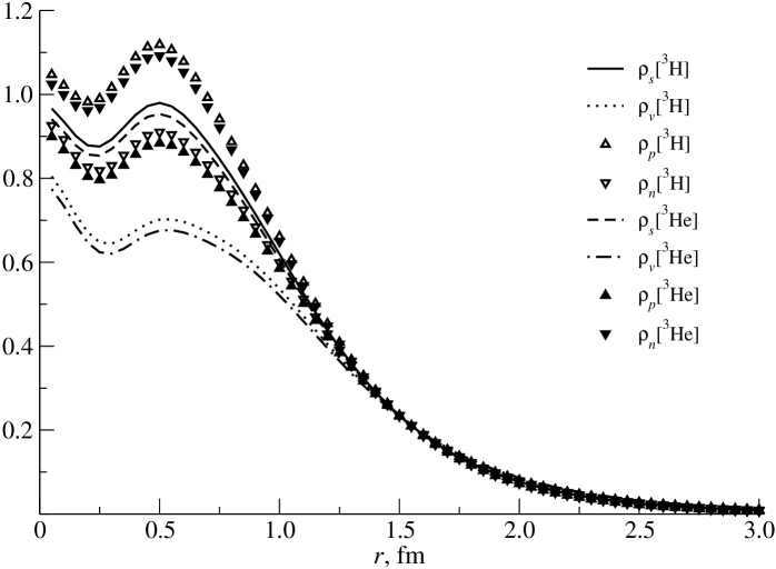
0mm flushleft

Figure 5: The isoscalar $\rho_{s}$, isovector $\rho_{v}$, proton $\rho_{p}$, and neutron $\rho_{n}$ densities in external $3N$ channel for ³H and ³He systems obtained with DBM (version I).

Below we present also two-proton density for ³He, which is defined usually as Doyle92 :

$$\rho_{pp}(r)=6\left\langle\Psi^{\rm ex}\left|\frac{\delta(r-r_{1})}{r^{2}}\frac{1+\tau_{3}^{(2)}}{2}\frac{1+\tau_{3}^{(3)}}{2}\right|\Psi^{\rm ex}\right\rangle.$$ (67)

This density is normalized to 2: $\int\rho_{pp}(r)r^{2}{d}r=2$. (As there is only a single nucleon in $6qN$ channel, we do not attach the index ‘‘ex’’ to this quantity.) The two-neutron density $\rho_{pp}(r)$ for ³H is defined similarly (with replacing $1+\tau_{3}^{(i)}\to 1-\tau_{3}^{(i)}$ in Eq. (67). In Fig. 6 we show both these densities for DBM(I) and also the two-proton density for ³He found with Bonn $NN$ potential Doyle92 .

0mm flushleft

Figure 6: The two-proton density in ³He (solid line) and two-neutron density in ³H (dashed line) calculated with DBM (version I) in comparison with two-proton density found with Bonn potential Doyle92 (triangles).

The internal $6qN$ channels. Here we define a density (normalized to unity) of the pure nucleon distributions as

$$\rho^{\rm in}_{\{{p\atop n}\}}(r)=\frac{1}{N^{\rm in}_{\{{p\atop n}\}}P_{\rm in}^{(1)}}{\left\langle\Psi^{\rm in}_{1}\left|\frac{\delta(r-\alpha\rho_{1})}{r^{2}}\frac{1\pm\tau_{3}^{(1)}}{2}\right|\Psi^{\rm in}_{1}\right\rangle},$$ (68)

where $P_{\rm in}^{(1)}=\langle\Psi^{\rm in}_{1}|\Psi^{\rm in}_{1}\rangle$ and the quantity

$$N^{\rm in}_{\{{p\atop n}\}}=\frac{1}{P_{\rm in}^{(1}}\left\langle\Psi^{\rm in}_{1}\left|\frac{1\pm\tau_{3}^{(1)}}{2}\right|\Psi^{\rm in}_{1}\right\rangle,$$ (69)

has the meaning of the average number of protons (neutrons) in the one internal $6qN$ channel (note that $N_{p}^{\rm in}+N_{n}^{\rm in}=1$, i.e., there is only one nucleon in each internal channel). The number $N^{\rm in}_{\{{p\atop n}\}}$ depends on ratio of norms of $6qN$ components with different values of isospin of the bag. Therefore, the separation of the $6qN$-channel density into isoscalar and isovector parts has no meaning.

These average numbers of nucleons in $6qN$ channel can be expressed through relative probabilities of the $6qN$ components with definite value of isospin $t$, which in our case are equal to:

$$P^{\rm in}_{0}\equiv P^{\rm in}_{t=0}=P^{\rm in}_{S1}+P^{\rm in}_{D},$$

$$P^{\rm in}_{1}\equiv P^{\rm in}_{t=1}=P^{\rm in}_{S0},$$ (70)

where $P^{\rm in}_{S1}$, $P^{\rm in}_{D}$, and $P^{\rm in}_{S0}$ are determined by Eq. (53). Hence, $P^{\rm in}_{t=0}+P^{\rm in}_{t=1}=1$. Then one can write down the average numbers of nucleons as

$$N^{\rm in}_{p}(^{3}{\rm H})=N^{\rm in}_{n}(^{3}{\rm He})=\frac{2}{3}P^{\rm in}_{t=1},$$

$$N^{\rm in}_{p}(^{3}{\rm He})=N^{\rm in}_{n}(^{3}{\rm H})=P^{\rm in}_{t=0}+\frac{1}{3}P^{\rm in}_{t=1}.$$ (71)

The nucleon densities (61) can be expressed by similar formula through components of the internal wavefunction with definite value of isospin $t$.

The total densities of nucleon distributions. The total nucleon densities (normalized to unity) for whole $3N$ system with allowance for both the $3N$ and $6qN$ components can be now defined as

$$\rho_{\{{p\atop n}\}}=\frac{(1-P_{\rm in})\rho^{\rm ex}_{\{{p\atop n}\}}N_{\{{p\atop n}\}}+P_{\rm in}\rho^{\rm in}_{\{{p\atop n}\}}N^{\rm in}_{\{{p\atop n}\}}}{\langle N_{\{{p\atop n}\}}\rangle},$$ (72)

where $P_{\rm in}={3P^{\rm in}_{1}}/(1+3P^{\rm in}_{1})$ is the total weight of all three internal channels (Eq. (54)) and the denominator:

$$\langle N_{\{{p\atop n}\}}\rangle=(1-P_{\rm in})N_{\{{p\atop n}\}}+P_{\rm in}N^{\rm in}_{\{{p\atop n}\}}<N_{\{{p\atop n}\}}$$ (73)

is equal to the average number of protons (neutrons) in the whole multicomponent system. The densities of the total proton and neutron distributions and also external- and internal-channel distributions for ³He calculated for DBM(i) are presented in Fig. 7.

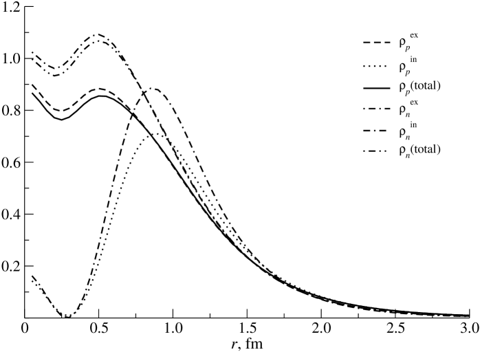
0mm flushleft

Figure 7: The external $\rho^{\rm ex}$, internal $\rho^{\rm in}$, and total $\rho(\rm total)$ densities of proton- and neutron distributions in ³He found with DBM (version I).

One can define also a (normalized) density of the matter (or mass) distribution in the $6qN$ channel as:

$$r^{2}\rho^{\rm in}_{m}(r)=\frac{1}{(m_{N}+m_{d})\,P_{\rm in}}{\langle\Psi^{\rm in}_{1}|{\delta(r-\alpha\rho_{1})}m_{N}+\delta(r-(1-\alpha)\rho_{1})m_{d}|\Psi^{\rm in}_{1}\rangle},$$ (74)

where $\alpha={m_{d}}/(m_{d}+m_{N})$, $m_{N}$ is a nucleon mass, and $m_{d}$ is mass of the bag (dibaryon). Then the total matter density (normalized to unity) is equal to

$$r^{2}\rho_{m}(r)=\frac{(1-P_{\rm in})\rho^{\rm ex}_{m}3m_{N}+P_{\rm in}\rho^{\rm in}_{m}(m_{N}+m_{d})}{\langle m\rangle}.$$ (75)

The r.m.s. radius of any distribution normalized to unity is defined by Eq. (65). The denominator in Eq. (75) determines the average mass of the whole system with taking into account non-nucleonic channels:

$$\langle m\rangle=(1-P_{\rm in})3m_{N}+P_{\rm in}(m_{N}+m_{d})=3m_{N}+P_{\rm in}(m_{d}-2m_{N})>3m_{N}.$$ (76)

0mm flushleft

Table 3: Isospin structure of $6qN$ channel, average number of nucleons and average mass calculated with the ground state wavefunctions of ³H and ³He in the DBM approach

	3H		3He
	DBM(I)	DBM(II)	DBM(I)	DBM(II)
$P^{\rm in}_{t=1}$	0.6004	0.6005	0.6044	0.6044
$P^{\rm in}_{t=0}$	0.3996	0.3995	0.3956	0.3956
$3N^{\rm in}_{p}$	0.799	0.799	2.209	2.209
$3N^{\rm in}_{n}$	2.201	2.201	0.791	0.791
$\langle N_{p}\rangle$	0.919	0.945	1.863	1.908
$\langle N_{n}\rangle$	1.861	1.906	0.920	0.947
$\langle N\rangle$	2.780	2.852	2.784	2.855
$\langle m\rangle/3m_{N}$	1.015	1.010	1.014	1.010

In the Table 3 we present some characteristics of isospin structure for wavefunctions in the $6qN$ channel: the relative probabilities for the components with $t=0$ and $t=1$ (i.e., $P^{\rm in}_{t=0}$ and $P^{\rm in}_{t=1}$), average numbers of protons and neutrons in all three $6qN$ components ($3\langle N_{\{{p\atop n}\}}\rangle$), and also the average number of nucleons $\langle N\rangle$ and the average mass $\langle m\rangle$ (divided by $3m_{N}$ value) in the whole four-component $3N$ system. It should be noted that the average number of nucleons in our multicomponent model, $\langle N_{\{{p\atop n}\}}\rangle$, is always less than the numbers of nucleons in $3N$ channel just due to existence of the non-nucleonic components. For example for DBM(I), the average number of protons in ³H is approximately equal to the average number of neutrons in ³He, viz. $\langle N_{p}\rangle(^{3}{\rm H})\approx\langle N_{n}\rangle(^{3}{\rm He})$, and is equal 0.92 while the average number of neutrons in ³H is approximately equal to the average number of protons in ³He, viz. $\langle N_{n}\rangle(^{3}{\rm H})\approx\langle N_{p}\rangle(^{3}{\rm He})$, and is equal 1.86. Hence the average number of nucleons found with the total multicomponent ³H and ³He functions is also always less than 3:

$$\langle N\rangle=\langle N_{p}\rangle+\langle N_{n}\rangle=3-2P_{\rm in}<3.$$

In our DBM, $\langle N\rangle$ is equal 2.78 and 2.85 for versions I and II, respectively.

The charge distributions. The charge distribution for the point-like particles in the $6qN$ channel can be written as the charge density of a system consisting of a point-like nucleon and a point-like bag:

$$r^{2}\rho^{\rm in}_{\rm ch-point}(r)=\frac{1}{Z}{\left\langle\Psi^{\rm in}_{1}\left|{\delta(r-\alpha\rho_{1})}\frac{1+\tau_{3}^{(1)}}{2}+\delta(r-(1-\alpha)\rho_{1})(1+\hat{t}_{3})\right|\Psi^{\rm in}_{1}\right\rangle},$$ (77)

where $1+\hat{t}_{3}$ is operator of the bag charge. The total charge radius in $6qN$ channel includes the r.m.s. radius of this point-like distribution $\langle r^{2}\rangle^{\rm in}_{\rm ch-point}$, the nucleon charge radius ($R_{p}$ or $R_{n}$) and the charge bag radius $R_{d}$, which depends on the bag isospin $t$ and its projection $t_{3}$:

$$\langle r^{2}\rangle^{\rm in}_{\rm ch}=\langle r^{2}\rangle^{\rm in}_{\rm ch-point}+\frac{1}{Z}\left(N^{\rm in}_{p}R^{2}_{p}+N^{\rm in}_{n}R^{2}_{n}+{\left\langle\Psi^{\rm in}_{1}\left|\sum_{t,t_{3}}\Gamma_{t,t_{3}}R^{2}_{d}(t,t_{3})\right|\Psi^{\rm in}_{1}\right\rangle}\right).$$ (78)

The last term in Eq. (78) includes the projectors $\Gamma_{t,t_{3}}$ onto the $6q$ bag isospin state with definite values of isospin $t$ and its projection $t_{3}$ and is equal to (for the ³H and ³He states with total isospin $T=1/2$):

$$\Delta(r^{2}_{\rm ch})^{\rm in}_{\rm bag}=\frac{1}{Z}\left\{R^{2}_{d}(0,0)P^{\rm in}_{t=0}+\left(\frac{1}{3}R^{2}_{d}(1,0)+\frac{2}{3}R^{2}_{d}(1,1)\delta_{T_{3},\frac{1}{2}}+\frac{2}{3}R^{2}_{d}(1,-1)\delta_{T_{3},-\frac{1}{2}}\right)P^{\rm in}_{t=1}\right\}.$$ (79)

The own charge radius of the $6q$ bag $R^{2}_{d}(t,t_{3})$ has, in general, different values in different isospin states, (which is related to the different multiquark dynamics in the channels with different isospin values) but we suppose in this work that their difference can be ignored, viz.

$$R^{2}_{d}(0,0)=R^{2}_{d}(1,0)=R^{2}_{d}(1,1)=R^{2}_{d}=b_{0}^{2},\qquad b_{0}=0.6\mbox{ fm},$$

$$\mbox{and }R^{2}_{d}(1,-1)=0\qquad(\mbox{which corresponds to a $nn$-bag}).$$ (80)

With the above assumptions the $6q$ bag contribution to the ³H and ³He charge radius is reduced to:

$$\Delta(r^{2}_{\rm ch})^{\rm in}_{\rm bag}=\frac{R^{2}_{d}}{Z}\left(P^{\rm in}_{0}+\frac{2+2T_{3}}{3}P^{\rm in}_{1}\right).$$ (81)

The r.m.s. charge radius of whole multicomponent system is defined as:

$$r^{2}_{\rm ch}=(1-P_{\rm in})\langle r^{2}\rangle_{\rm ch}^{\rm ex}+P_{\rm in}\langle r^{2}\rangle_{\rm in}^{\rm ex}.$$

0mm flushleft

Table 4: The total r.m.s. radii (in fm) for the proton ($r_{p}$), neutron ($r_{n}$), matter ($r_{m}$), and charge ($r_{\rm ch}$) distributions in DBM approach and their separate values for external and internal channels

Model		3H				3He
		$r_{p}$	$r_{n}$	$r_{m}$	$r_{\rm ch}$	$r_{p}$	$r_{n}$	$r_{m}$	$r_{\rm ch}$
DBM(I)	$3N$	1.625	1.770	1.723	1.779	1.805	1.648	1.754	1.989
	$6qN$	1.608	1.823	1.142	1.188	1.854	1.618	1.159	1.412
	Total	1.625	1.773	1.663	1.724	1.807	1.647	1.694	1.935
DBM(II)	$3N$	1.613	1.761	1.713	1.769	1.795	1.636	1.744	1.980
	$6qN$	1.573	1.797	1.124	1.171	1.829	1.583	1.141	1.396
	Total	1.613	1.762	1.672	1.732	1.796	1.635	1.703	1.944
AV18 + UIX(a)		1.59	1.73			1.76	1.61
Experiment		1.60(b)			1.755	1.77(b)			1.95

^a)Taken from Pieper .

^b)These ‘‘experimental’’ values are taken from Pieper . They have been obtained by substraction of the own proton and neutron charge radii squared (0.743 and –0.116 fm², respectively) from the experimental values of the charge radii squared.

In the Table 4 we give r.m.s. radii for all the above distributions in ³H and ³He found in the impulse approximation, as well as the respective experimental values and results obtained for AV18($2N$) + UIX($3N$) forces. To demonstrate the separate contributions of the $3N$ and $6qN$ channels to these observables, we also present the values calculated separately with only nucleonic and $6qN$ parts of the total wavefunction. It is seen from the Table 4 that both versions of our model (viz. DBM(I) and DBM(II)) give quite similar values for all the radii. The most interesting point here is the importance of $6qN$ component contributions. In fact, the contribution of the $6qN$ channel shifts all the radii, i.e., $r_{\rm ch}$ and $r_{p}$ in ³H and ³He, predicted with pure nucleonic components in our approach, much closer to the respective experimental values. For example, the value $r_{\rm ch}=1.822$ fm calculated for ³H with only the nucleonic part of the wavefunction is essentially larger than the respective experimental value 1.755 fm. However, an admixture of a rather compact $6qN$ component ($r_{\rm ch}=1.22$ fm) immediately shifts the ³H charge radius down to a value of 1.766 fm, which is very close to its experimental value.

Thus, the dibaryon–nucleon component works in a right way also in this aspect. It is interesting to note that, in general, the predictions of our two-phase model are quite close to those of the conventional pure nucleonic AV18 + UIX model. This means that our multichannel model is effectively similar to a conventional purely nucleonic model (at least for many static characteristics). However, this similarity will surely hold only for the characteristics that are sensitive mainly to low-momentum transfers, while the properties and processes involving high-momentum transfers will be treated in two alternative approaches in completely different ways.

7.3 Coulomb displacement energy and charge symmetry breaking effects

The problem of accurate description of Coulomb effects in ³He in the current $3N$ approach of the Faddeev or variational type has attracted much attention for last three decades (see, e.g., Friar ; Gloeckle and the references therein to the earlier works). It is interesting that the Coulomb puzzle in ³He, being related to the long-range interactions, is treated in a different manner in our and conventional approaches.

The $\Delta E_{\rm C}$ problem dates back to the first accurate $3N$ calculations performed on the basis of the Faddeev equations with realistic $NN$ interactions in the mid-1970s Gignoux . These pioneer calculations first exhibited a hardly removable difference of ca. 120 keV between the theoretical prediction for $\Delta E_{\rm C}^{\rm th}\simeq 640$ keV and the respective experimental value $\Delta E_{\rm C}^{\rm exp}\simeq 760$ keV. In subsequent 30 years, numerous accurate $3N$ calculations have been performed over the world using many approaches, but this puzzle was still generally unsolved. The most plausible quantitative explanation (but yet not free of serious questions) for the puzzle has been recently suggested by Nogga et al. Gloeckle . They have observed that the difference in the singlet ${}^{1}S_{0}$ scattering lengths of $pp$ (nuclear part) and $nn$ systems (originating from the effects of charge symmetry breaking (CSB)) can increase the energy difference between ³H and ³He binding energies and thus contribute to $\Delta E_{\rm C}$.

Our results obtained in this work with DBM give an alternative explanation of the $\Delta E_{\rm C}$ puzzle and other Coulomb effects in ³He without any free parameter. The Coulomb displacement energies $\Delta E_{\rm C}$, together with the individual contributions to the $\Delta E_{\rm C}$-value, are presented in Table 5.

0mm flushleft Contribution DBM(I) DBM(II) AV18 + UIX Point Coulomb $3N$ only 598 630 677 Point Coulomb $3N+6qN$ 840 782 – Smeared Coulomb $3N$ only 547 579 648 Smeared Coulomb $3N+6qN$ 710 692 – $np$ mass difference 46 45 14 Nuclear CSB (see Table 6) 0 0 +65 Magnetic moments and spin-orbit^a) 17 17 17 Total 773 754 754

Table 5: Contribution of various terms (in keV) of the Coulomb interaction to the ³H–³He mass difference $\Delta E_{\rm C}$

^a)Here we use the value for this correction from Gloeckle .

We emphasize three important points, where our results differ from those for conventional models.

• First, we found a serious difference between conventional and our approaches in the short-range behavior of wavefunctions even in the nucleonic channel. Conventional $3N$ wavefunctions are strongly suppressed along all three interparticle coordinates $r_{ij}$ due to the short-range local repulsive core, while our wavefunctions (in the $3N$ channel) have stationary nodes and short-range loops along all $r_{ij}$ and the third Jacobi coordinates $\rho_{k}$. Such a node along the $\rho$ coordinate is seen also in the $6qN$ relative-motion wavefunction. This very peculiar short-range behavior of our wavefunctions leads to a strong enhancement of the high-momentum components of nuclear wavefunctions, which is required by various modern experiments. On the other hand, these short-range radial loops lead to significant errors, when using the Coulomb interaction between point-like particles within our approach. Hence, we must take into account the finite radii of charge distributions in the proton and $6q$ bag. Otherwise, all Coulomb energies will be overestimated.

• Another important effect following from our calculations is a quite significant contribution of the internal $6qN$ component to $\Delta E_{\rm C}$. In fact, just this interaction, which is completely missing in conventional nuclear force models, makes the main contribution (163 and 113 keV for versions I and II correspondingly) to filling the gap in $\Delta E_{\rm C}$ between conventional $3N$ calculations and experiment if the CSB effects are of little significance in $\Delta E_{\rm C}$.

  The large magnitude of this three-body Coulomb force contribution in our models can be explained by two factors: first, a rather short average distance $\langle\rho^{2}\rangle^{1/2}$ between the $6q$ bag and the third nucleon (which enhances the Coulomb interaction in the $6qN$ channels) and, second, a relatively large weight of the $6qN$ components, where the $6q$ bag has the charge +1 (i.e., it is formed from $np$ pair). This specific Coulomb repulsion in the $6qN$ channel should appear also in all other nuclei, where the total weight of such components is about 10% and higher. Therefore, it should strongly contribute to the Coulomb displacement energies over the entire periodic table and could somehow explain the long-term Nolen–Schiffer paradox Nollen in this way.

• The third specific effect that has been found in this study and contributes to the quantitative explanation of $\Delta E_{\rm C}$ is a strong increase in the average kinetic energy $\langle T\rangle$ of the system. This increase in $\langle T\rangle$ has been already discovered in the first early $3N$ calculations with the Moscow $NN$ potential model Tur2 and results in a similar nodal wavefunction behavior along all interparticle coordinates but without any non-nucleonic component.

  The increase in $\langle T\rangle$ leads to the proportional increase in the $np$ mass difference correction to $\Delta E_{\rm C}$. Since the average kinetic energy in our case is twice the kinetic energy in conventional force models, this correction is expected to be also much larger in our case. Hence, we evaluate such a correction term in the following way (without usage of the perturbation theory). In the conventional isospin formalism, one can assume that the ³H and ³He nuclei consist of the equal-mass nucleons:

  $${m}=\frac{m_{p}+m_{n}}{2},$$

  so that $m_{p}=m+\Delta m/2,\;m_{n}=m-\Delta m/2$, where $\Delta m=m_{p}-m_{n}$. The simplest way to include the correction due to the mass difference $\Delta m$ is to assume that all particles in ³H have the average mass

  $$\bar{m}_{\rm H}=\frac{2m_{n}+m_{p}}{3}=m-\frac{1}{6}\Delta m,$$

  while in ³He they have the different average mass

  $$\bar{m}_{\rm He}=\frac{2m_{p}+m_{n}}{3}=m+\frac{1}{6}\Delta m.$$

  In spite of smallness of the parameter $\Delta m/m$, the perturbation theory in respect of this parameter does not work. So we used the average mass $\bar{m}_{\rm H}$ in calculation of ³H and $\bar{m}_{\rm He}$ in calculation of ³He. The contribution of this $np$ mass difference to the $\Delta E_{\rm C}$ value is given in the fifth row of Table 5. As is seen from the table, this correction is not very small in our case and contributes to $\Delta E_{\rm C}$ quite significantly.

  Many other effects attributed to increasing the average kinetic energy of the system will arise in our approach, e.g., numerous effects associated with the enhanced Fermi motion of nucleons in nuclei.

Charge symmetry breaking effects in DBM. As was noted above, the best explanation for the $\Delta E_{\rm C}$ value in the framework of conventional force models published up to date Gloeckle is based on the introduction of some CSB effect, i.e., the difference between $nn$ and $pp$ strong interactions. At present, two alternative values of the $nn$ scattering length are assumed:

$$a^{(1)}_{nn}=-18.7\mbox{ fm and }a^{(2)}_{nn}=-16.3\mbox{ fm}.$$ (82)

The first value has been extracted from the previous analysis of experiments $d(\pi^{-},\gamma)nn$ dpigam (see also dpig1 and references therein) and is used in all current $NN$ potential models, while the second value in (82) has been derived from numerous three-body breakup experiments $n+d\to nnp$ done for the last three decades. In recent years, such breakup experiments are usually treated in the complete Faddeev formalism, which includes most accurately both two-body and 3BF a16 . Thus, this $a^{(2)}_{nn}$ value is considered as a quite reliable one. However, the quantitative explanation for the $\Delta E_{\rm C}$ value in conventional force models uses just the first value of $a_{nn}$ as an essential point of all the construction. At the same time, the use of the second value $a_{nn}(=-16.3\mbox{ fm})$ (which is not less reliable than the first one) invalidates completely the above explanation!

Therefore, in order to understand the situation more deeply and to determine the degree of sensitivity of our prediction for $\Delta E_{\rm C}$ to variation in $a_{nn}$, we made also $3N$ calculations with two possible values of $a_{nn}$ from Eq. (82). These calculations have been carried out with the effective values of the singlet-channel coupling constant corresponding to the $V_{NqN}$ part of the $NN$ force:

$$\lambda^{\rm eff}_{{}^{3}{\rm He}}(^{1}S_{0})=\frac{1}{3}\lambda_{pp}+\frac{2}{3}\lambda_{np},$$ (83)

$$\lambda^{\rm eff}_{{}^{3}{\rm H}}(^{1}S_{0})=\frac{1}{3}\lambda_{nn}+\frac{2}{3}\lambda_{np}.$$ (84)

In the above calculations, we employ the value $\lambda_{np}=328.9$ MeV that provides the accurate description of the ${}^{1}S_{0}$ $np$ phase shifts and the experimental value of the $np$ scattering length $a_{np}=-23.74$ fm KuInt . Here, for $pp$-channel we use the value $\lambda_{pp}=325.523$ MeV fitted to the well-known experimental magnitude $a_{pp}=-8.72$ fm and for $nn$-channel two $\lambda_{nn}$ values corresponding to two available alternative values of the $nn$ scattering length (82) have been tested. The calculation results are presented in Table 6.

0mm flushleft

Table 6: Contribution of charge symmetry breaking effects to the ³H–³He mass difference $\Delta E_{\rm C}$

	$\Delta E_{\rm C}$, keV
$a_{nn}$, fm	DBM(I)	DBM(II)
–16.3	–18	–39
–18.9	+45	+26

As is seen in Tables 5 and 6, the DBM (version I) can precisely reproduce the Coulomb displacement energy $\Delta E_{\rm C}$ with the lower (in modulus) value $a_{nn}=-16.3$ fm, while this model overestimates $\Delta E_{\rm C}$ by 54 keV (=45 + 9 keV) with the larger (in modulus) value $a_{nn}=-18.9$ fm. Thus, the DBM approach, in contrast to the conventional force models, prefers the lower (in modulus) possible value –16.3 fm of the $nn$ scattering length, which has been extracted from very numerous $3N$ breakup experiments $n+d\to nnp$ a16 .

Now, let us discuss shortly the magnitude of CSB effects in our model. The measure of CSB effects at low energies is used to consider the difference between $a_{nn}$ and so-called ‘‘pure nuclear’’ $pp$ scattering length $a_{pp}^{N}$ that is found from $pp$ scattering data, when the Coulomb potential is disregarded. The model dependence of the latter quantity was actively discussed in the 1970s–1980s SauWall ; Rahman ; Albev . However, the majority of modern $NN$ potentials fitted to the experimental value $a_{pp}=-8.72$ fm results in the value $a^{N}_{pp}=-17.3$ fm, when the Coulomb interaction is discarded. It is just the value that is adopted now as an ‘‘empirical’’ value of the $pp$ scattering length Machl . Thus, the difference between this value and $a_{nn}$ is usually considered as the measure of CSB effects. However, our model (also fitted to the same experimental value $a_{pp}=-8.72$ fm) gives a quite surprising result:

$$a^{N}_{pp}({\rm DBM})=-16.57\mbox{ fm},$$ (85)

which differs significantly from the above conventional value (by 0.8 fm) due to the explicit energy dependence of the $NN$ force in our approach.

Thus, if the difference $a^{N}_{pp}-a_{nn}$ is still taken as the measure of CSB effects, the smallness of this difference obtained in our model testifies to a small magnitude of the CSB effects, which is remarkably smaller than the values derived from conventional OBE models for the $NN$ force.

8 Discussion

The $3N$ results presented in the previous section differ significantly from the results found with any conventional model for $NN$ and $3N$ forces (based on Yukawa’s meson exchange mechanism) and also from the results obtained in the framework of hybrid models hyb , which include the two-component representation of the $NN$ wavefunction $\Psi=\Psi_{NN}+\Psi_{6q}$. It is convenient to discuss these differences in the following order.

• We found that the $q^{2}$ dependence of pair $NN$ forces on the momentum of the third particle in the $3N$ system is more pronounced in our case than in other hybrid models hyb ; Bakk ; Weber ; Sim : the $3N$ binding energy decreases by ca. 1.7 MeV, from 5.83 to 4.14 MeV when one takes into account the $q^{2}$-dependence (cf. the first and second rows in Table 2). From more general point of view, it means that, in our approach, pairwise $NN$ interactions (except Yukawa OPE and TPE terms), being ‘‘embedded’’ into a many-body system, loose their two-particle character and become substantially many-body forces (i.e., depending on the momenta of other particles of the system).

• Due to such a strong $q^{2}$ dependence (of ‘‘repulsive’’ character), the $3N$ system calculated including only the pairwise forces turns out to be strongly underbound ($E=-4.14$ MeV). In other words, the ‘‘pairwise’’ $NN$ forces (including their $q^{2}$ dependence on the momenta of the third nucleon) give only about half the total $3N$ binding energy, leaving the second half for the 3BF contribution. Therefore, the following question is decisively important: can the 3BF (inevitably arising in our approach) give the large missing contribution to the $3N$ binding energy? Usefulness of the developed model for the description of nuclear systems depends directly on the answer to this important question. It is appropriate here to remind that in the conventional 3BF models such as Urbana–Illinois or Tucson–Melbourne, the contribution of 3BF to the total $3N$ binding energy does not exceed 1 MeV; i.e., this contribution can be considered as some correction ($\sim 15$%), although it is significant for the precise description of the $3N$ system.

• Fortunately, the contribution of 3BF induced by OSE and TSE enables one to fill this 4.3 MeV gap between the two-body force contribution and experimental value. In fact, including both OSE and TSE contributions to 3BF, taken with the same coupling constants and form factors as in the driving $NN$-force model, together with a quite reasonable value for the $\sigma NN$ coupling constant, $g_{\sigma NN}=8$–10, one obtains the $3N$ binding energy that is very close to the experimental value (see rows 3, 4 and 6, 7 in Table 2). Thus, the presented force model leads to a very reasonable binding energy for the $3N$ system, however, with the murch larger (as compared to the traditional $3N$ force model) contribution of 3BF. In fact, the unification of the basic $2N$ and $3N$ force parameters provides a strong support for the whole force model suggested here and is in a sharp contrast with all traditional force model based on $t$-channel exchange mechanism. We remind to reader that the $2N$ and $3N$ forces in conventional approaches (where the latter is induced by an intermediate $\Delta$-isobar production) are taken with different cut-off parameters values $\Lambda_{\pi NN}$ and $\Lambda_{\pi N\Delta}$ in $2N$ and $3N$ sectors in order to explain the basic features of $3N$ nuclei and $N+d$ scattering! Thus in the traditional approach, one has some serious inconsistency in parameter values for $2N$ and $3N$ sectors.

• The contributions of the pairwise and different three-body forces to the total $3N$ binding energy for ³H are given in the fifth and sixth rows of Table 2. From the results presented in this table, one can conclude that just the total 3BF contribution to the $3N$ binding energy dominates and, in fact, determines the whole structure of the ³H and ³He ground states. Moreover, comparing the third and fourth rows of the table, one can see a ‘‘nonlinear’’ effect of self-strengthening for the 3BF contribution. In fact, the comparison of the results presented in these rows of the table (see the second and the fifth columns) shows clearly that the binding energy is almost proportional to the weight $P_{\rm in}$ of the $6qN$ component in the total $3N$ wavefunction. Thus, when the weight of the $6qN$ component increases, the 3BF contribution, which is related directly only to this component of the total wavefunction, increases accordingly. However, the enhancement of the pure attractive 3BF contribution squeezes the $3N$ system and thus reduces its r.m.s. radius, i.e., the mean distance between nucleons, which, in turn, again increases the weight of the $6qN$ component. In other words, a some chain process which strengthens the attraction in the system arises. This process is balanced both by the weakening of the effective pairwise interaction due to the $q^{2}$ dependence and by the repulsive effect of the orthogonalizing pseudopotentials included in each pair interaction.

  There are two another important stabilizing factors weakening the strong three-body attraction in the $3N$ system. First, the generation of the short-range repulsive vector $\omega$-field, where all three nucleons are close to each other Bled . Since the $\omega$-meson is heavy, this field is located in the deep overlap region of all three nucleons. In the present study, we omitted the three-body contribution of this repulsive $\omega$-field. This repulsive contribution will keep the whole system from the further collapse due to the strong attractive $3N$ force induced by the scalar field.

  The second factor weakening slightly the effective $3N$ attraction is associated with the conservation of the number of scalar mesons generated in the $2N$ and $3N$ interaction process. The problem is that TSE giving the 3BF contribution (see Fig. 4) arises due to the break of the $\sigma$-meson loop, which induces the main $2N$ force. In other words, the $\sigma$ meson generated in the transition of pair nucleons from the $NN$ phase state to the $6q$ state is absorbed either in the $6q$ bag with closing the loop or by the third nucleon, resulting in the 3BF contribution. Thus, the appearance of such a 3BF should weaken the attraction between nucleons in the pair. We carefully estimated the effect of the meson-number conservation for the TSE contribution on the total $3N$ binding energy. Its magnitude occurred to be rather moderate in the absolute energy scale (ca. 0.3–0.4 MeV), but quite noticeable within the whole TSE contribution. However, when the total nucleon density increases (and the relative TSE contribution also increases), the effect is enhanced.

• Dependence of the two-body coupling constants $\lambda(\varepsilon)$ upon the average momentum of other nucleon in $3N$ system (see, e.g., Eq. (29)) can be interpreted generally as a density dependence of the resulted many-body force in many-nucleon system. It is easy to show the appearance of the energy-dependent pairwise potentials of the above-mentioned type leads inavoidably to a repulsive many-body force. In other words, the effects of the two-body interactions of this type can be reinterpeted in terms of the conventional static interaction as additional contribution of the effective repulsive density-dependent many-body force. For example, if to remove the $q^{2}$-dependence from the coupling constant $\lambda(E-q^{2}/2m)$ of our two-body force (this $q^{2}$-dependence leads to a weakening of the two-body force in a many-nucleon system, when $q^{2}$ is rising), then the neglected $q^{2}$-dependence must be compensated by an additional repulsive density-dependent effective three-body force. Thus we can replace this energy-dependent two-body interaction by an effective static two-body potential (as it is usually done) plus a repulsive density-dependent 3BF.

  On the other hand, it is well known from the Skirme-model calculations of nuclei that just similar repulsive phenomenological density-dependent 3BF should be added to conventional $2N$- and $3N$-forces to guarantee the saturation properties of heavy nuclei. Thus, in this respect the present force model is also in a qualitative agreement with phenomenological picture of nuclear interactions.

9 Conclusion

In this paper, we have developed a general formalism for the multicomponent description of the three-body system with particles having inner degrees of freedom. We have applied our new approach to studying $3N$ system with $2N$ and $3N$ interactions based on the dressed dibaryon intermediate state and $\sigma$-field generation. It has been shown that the DBM applied to the $3N$ system results inevitably in new three-body scalar and also new (three-body) Coulomb forces due to the (strong + Coulomb) interaction between the dressed dibaryon and the third nucleon. These forces play a crucial role in the structure of few-nucleon systems and very likely in whole nuclear dynamics. Our accurate variational calculations have demonstrated that new 3BF gives a half of the $3N$ binding energy, whereas the 3BF contribution in the traditional $NN$-force approaches gives about 15% of the total binding energy. Thus, the suggested approach to the $NN$ and $3N$ interactions can lead to significant revision of relative contributions of two- and many-body forces in all nuclear systems.

The developed model gives the precise value for the Coulomb displacement energy $\Delta E_{\rm C}$ of the $A=3$ system. Two basic sources of this contribution, which differ from conventional force models, should be indicated here:

• the three-body Coulomb force between the dressed bag and the charged third nucleon; and

• quite significant correction to the kinetic energy of the system due to the $np$ mass difference and high average kinetic energy.

It should be emphasized that, contrary to other studies based on conventional force models (using the $2N$ and $3N$ forces generated via the meson-exchange mechanism), this explanation does not require any noticeable CSB effect, although our model is still compatible with such effects. However, these CSB effects do not contribute remarkably to $\Delta E_{\rm C}$ in our approach.

It is crucially important that the DBM leads to a significant non-nucleonic components in the $3N$ wavefunction (8–11%), while this component in the deuteron is ca. 3%, which results in a reformulation of many basic effects in few-nucleon systems and other nuclei as well. It is probable that the weight of such non-nucleonic components in heavy nuclei can be even higher with an increase in the mass number and nuclear density.

There is a very specific new interplay between two- and three-body forces: the stronger the three-body force, the smaller the attractive contribution of the two-body force to the nuclear binding energy! This gives a very important stabilization in nuclei and nuclear matter. By this way, a very natural density dependence of nuclear interactions appears from the beginning. Thus, the general properties of the $3N$ system, where forces so much differ from any conventional force model, would appear also to be much differ from the predictions of any conventional model and, hence, from experiment.

Therefore, it was very surprising for us to find that the static characteristics of the $3N$ system in our case turned out to be very close to the predictions of the modern force model (such as AV18 + UIX) and thus to experiment. This gives us a good test of the self-consistency and accuracy of the new force model. However, predictions of the present $NN$- and $3N$-force model in other aspects will strongly be deviated from those for conventional models. First, these are the properties determined by the high-momentum components of nuclear wavefunctions. The point is that the system described by our multicomponent wavefunctions including the dibaryon components explicitly can easily absorb high-momentum transfers, which can hardly be absorbed by the system consisting of nucleons only. Therefore, to fit the experimental data corresponding to large-momentum transfers ($\sim 1\mbox{ GeV}/c$), many types of meson-exchange and isobar currents are often introduced into theoretical frameworks. However, these currents are often unrelated to the underlying force model. Hence, it is rather difficult to check the self-consistency of such calculations, e.g., the validity of gauge invariance, etc.

Numerous modern experiments could corroborate these results. In particular, according to the recent experiments ${}^{3}{\rm He}(e,e^{\prime}pp)$ Nikef and their theoretical interpretation on the basis of fully realistic $3N$ calculations, the cross sections for the ${}^{3}{\rm He}(e,e^{\prime}pp)$ process are underestimated by about five times with a fully realistic $3N$ model and incorporation of final state interaction and meson-exchange currents. This important conclusion has been further confirmed in recent experiments at the Jefferson Laboratory when the incident electron beam energy has been increased up to $E_{e}=2.2$ and 4.4 GeV Jef . The data of the two different experiments give a clear evidence of very strong short-range $NN$ correlation in the ³He ground state. This correlation still cannot be explained within the traditional pattern for the $3N$ system.

In addition, our approach has recently been partially supported Kask from the other side by considering a model for $2\pi$ production in $pp$ collisions at $E_{p}=750$ and 900 MeV. The authors have found that almost all particle energy and angular correlations (e.g., $\pi^{+}\pi^{-},\,pp,\,\pi pp$, etc.) can be explained quantitatively by assuming that $\pi^{+}\pi^{-}$ production occurs through the generation of an intermediate light $\sigma$ meson with the mass $m_{\sigma}\simeq 380$ MeV. These values generally agree with the parameters adopted in our $NN$ model KuJPG ; KuInt and drastically disagree with the values assumed in OBE and other potential models.

Very interesting general implication of the results presented here is their evident interrelation to the famous Walecka hadrodynamic model for nuclei Walecka . It is well known that the Walecka model describes nuclei and nuclear matter in terms of the scalar $\sigma$- and vector $\omega$-fields, where the $\sigma$-field gives the attractive contribution, while the vector $\omega$-field balances this attraction by short-range repulsion. It is very important that both basic fields appear (in the model) as the explicit degrees of freedom (together with relativistic nucleons), in contrast to conventional meson-exchange models for nuclear forces, where mesons appear as the carriers of forces rather than as the explicit field degrees of freedom. Our approach does include the $\sigma$-meson (and potentially the $\omega$-meson) degrees of freedom in an explicit form, similarly to the Walecka model. Moreover, since the average kinetic energy of the $3N$ system in our model is high (it is much higher than that in the conventional OBE approach), nucleon motion is closer to the relativistic case, and thus the similarity with the Walecka model gets even closer.

There is also an additional strong argument in favor of a tight interrelation between our and the above Walecka-type nuclear model. Very recently, we have formulated Shikh the dibaryon model for $NN$ interaction in terms of relativistic effective field theory with the intermediate dibaryon being represented as a color quantum string with color quark clusters at its ends. This theory includes $\pi$, $\sigma$, $\rho$ and $\omega$-mesons as a dressing of the dibarion together with the $N\Delta$ and $\Delta\Delta$ loops. Thus, the $3N$ scalar force introduced in the present work ‘‘by hands’’ can be derived in the field-theory Lagrange language within the effective field theory. Moreover, in the mean field approximation this effective field theory approach, being applied to nuclei, should result in the Walecka–Serot relativistic model with the dominating collective $\sigma$-field, which couples the nucleons in a nucleus together.

Thus, the alternative description given here by the new force model looks to be more self-consistent and straightforward than the conventional OBE-type models. One aspect of this new picture is evident – the present model being applied to any electromagnetic process on nuclei leads automatically to a consistent picture of the process as whole: single-nucleon currents at low-momentum transfers, meson-exchange currents (including new meson currents) at intermediate-momentum transfers, and quark counting rules at very-high-momentum transfers, because the model wavefunction includes explicitly multinucleon, meson-exchange, and multiquark components.

From all the above-mentioned arguments one can conclude that the dibaryon concept of nuclear force advocated in the work results in a new picture for nuclear structure and dynamics.

We are grateful to Dr. I. Obukhovsky for discussions and help in calculation of some matrix elements, and also to many our colleagues in Tübingen University for continuous encouraging in the course of this work, and also to the staff of Institut für Theoretische Physik der Universität Tübingen, where the most part of calculations has been performed.

This work was supported in part by der Deutsche Forschungsgemeinschaft (grant no. 436 RUS 113/790) and the Russian Foundation for Basic Research (grants nos. 02-02-16612, 04-02-04001).

APPENDIX

Overlap functions between $3N$ symmetrized basis and $NN$ form factors and matrix elements of DBM interactions for a $3N$ system

1 The construction of basis functions

The total wavefunction in $3N$ channel with the angular momentum $(J,M)$ and the isospin $(T,T_{z})$ is written as (below we omit the quantum numbers $JMTT_{z}$):

$$\Psi^{(JMTT_{z})}_{\rm ex}=\Psi^{(1)}_{\rm ex}+\Psi^{(2)}_{\rm ex}+\Psi^{(3)}_{\rm ex},$$ (1)

$$\Psi^{(i)}_{\rm ex}=\sum_{{\gamma},n}C^{\gamma}_{n}\Phi_{{\gamma}n}^{(i)}\qquad(i=1,2,3),$$ (2)

where

$$\Phi_{{\gamma}n}^{(i)}({\bf r}_{i},{\hbox{$\rho$}\hbox to0.0pt{\hss\hbox{$\rho$}\hskip 0.39993pt}\hbox to0.0pt{\hss\lower 0.17218pt\hbox{\hbox{$\rho$}\hbox to0.0pt{\hss\hbox{$\rho$}\hskip 0.39993pt}}}_{i}})=N^{\gamma}_{n}r_{i}^{\lambda}\rho_{i}^{l}\,\exp(-\alpha_{n}r_{i}^{2}-\beta_{n}\rho_{i}^{2}){\cal F}^{JMTT_{z}}_{{\gamma}}(\hat{\bf r}_{i},\hat{\hbox{$\rho$}\hbox to0.0pt{\hss\hbox{$\rho$}\hskip 0.39993pt}\hbox to0.0pt{\hss\lower 0.17218pt\hbox{\hbox{$\rho$}\hbox to0.0pt{\hss\hbox{$\rho$}\hskip 0.39993pt}}}}_{i})\,{\cal T}^{(i)}_{t_{jk}}.$$ (3)

We use the following notations: ${\bf r}_{i}$(${\bf p}_{i}$) is the relative coordinate (momentum) of the pair ($jk$), while ${\hbox{$\rho$}\hbox to0.0pt{\hss\hbox{$\rho$}\hskip 0.39993pt}\hbox to0.0pt{\hss\lower 0.17218pt\hbox{\hbox{$\rho$}\hbox to0.0pt{\hss\hbox{$\rho$}\hskip 0.39993pt}}}}_{i}$ (${\bf q}_{i}$) is the Jacobi coordinate (momentum) of the $i$th particle relative to the center of mass for the pair ($jk$), $(i,j,k)=(1,2,3)$ or their cyclic permutations. Here the composite label $\gamma=\{\lambda\,l\,L\,S_{jk}\,S\,t_{jk}\}$ represents the set of quantum numbers for the basis functions: the angular momenta $\lambda$ and $l$ correspond to the Jacobi coordinates ${\bf r}_{i}$ and ${\hbox{$\rho$}\hbox to0.0pt{\hss\hbox{$\rho$}\hskip 0.39993pt}\hbox to0.0pt{\hss\lower 0.17218pt\hbox{\hbox{$\rho$}\hbox to0.0pt{\hss\hbox{$\rho$}\hskip 0.39993pt}}}}_{i}$, respectively, $S_{jk}(t_{jk})$ is spin (isospin) of the two-body subsystem $(jk)$, and $L(S)$ is the total orbital momentum (spin) of the system. The normalizing coefficient in (A.3) is

$$N^{\gamma}_{n}=2^{\lambda+l+3}\sqrt{\frac{2\alpha_{n}^{\lambda+3/2}\beta_{n}^{l+3/2}}{\pi(2\lambda+1)!!(2l+1)!!}}.$$ (4)

The spin-angular ${\cal F}_{{\gamma}}$ and isospin ${\cal T}^{(i)}_{t_{jk}}$ parts of the basis function are defined by a standard vector-coupling scheme:

$${\cal F}^{JMTT_{z}}_{\gamma}=|\{\lambda_{i}l_{i}:L\}\{s_{j}s_{k}(S_{jk})s_{i}:S\}:JM\rangle,$$ (5)

$${\cal T}^{(i)}_{t_{jk}}=|t_{j}t_{k}(t_{jk})t_{i}:TT_{z}\rangle,$$ (6)

where $s_{i}(=1/2)$ and $t_{i}(=1/2)$ are spin and isospin of the $i$th nucleon.

Now we define the symmetrized basis functions as:

$$\Phi^{\rm sym}_{\gamma n}=\sum_{i=1,2,3}\Phi^{(i)}_{\gamma n},$$ (7)

so that the total wavefunction in an external ($3N$) channel takes the form:

$$\Psi_{\rm ex}=\sum_{{\gamma},n}C^{\gamma}_{n}\Phi_{{\gamma}n}^{\rm sym}.$$ (8)

2 Nucleon–nucleon form factors

The $NN$ form factors in the separable DBM interaction and in the projectors $\varphi^{J_{i}M_{i}t_{d}t_{d_{z}}}_{\lambda_{i}S_{d}}({\bf r}_{i})$, corresponding to the orbital momentum $\lambda_{i}$, spin $S_{d}$, the total angular momentum $(J_{i},M_{i})$, and isospin $(t_{d}t_{d_{z}})$ of the subsystem $(jk)$ ($\bf J_{i}={\hbox{$\lambda$}\hbox to0.0pt{\hss\hbox{$\lambda$}\hskip 0.39993pt}\hbox to0.0pt{\hss\lower 0.17218pt\hbox{\hbox{$\lambda$}\hbox to0.0pt{\hss\hbox{$\lambda$}\hskip 0.39993pt}}}}_{i}+S_{d}$), have the form:

$$\varphi^{J_{i}M_{i}t_{d}t_{d_{z}}}_{\lambda_{i}S_{d}}({\bf r}_{i})\equiv\varphi_{f}({\bf r}_{i})=\sum_{m}D^{f}_{m}r^{\lambda_{i}}_{i}\,\textstyle\exp(-\frac{1}{2}\eta^{2}_{m}r^{2}_{i})\,{\cal F}_{f}(\hat{\bf r}_{i})\,{\cal T}_{f}^{(i)},$$ (9)

where

$$f\equiv\{\lambda_{i},S_{d},J_{i},M_{i},t_{d},t_{d_{z}}\},\qquad{\cal F}_{f}=|\lambda_{i}S_{d}:J_{i}M_{i}\rangle,\qquad{\cal T}^{(i)}_{f}=|t_{j}t_{k}:t_{d}t_{d_{z}}\rangle,$$ (10)

and $D^{f}_{m}$ and $\eta_{m}$ are linear and nonlinear parameters, respectively, of the Gaussian expansion. (In this Appendix we have altered the notation for the quantum numbers of the $NN$ form factor as compared with the main text of the paper: we have replaced $L_{i}\to\lambda_{i}$ for the orbital momentum and also included the isospin quantum numbers $t_{d},t_{d_{z}}$.) In the single-pole approximation the DBM includes only one form factor for each set $f$, so that index $f$ determines the form factor uniquely. In the present version of DBM we use only $0S$, $2S$, and $2D$ oscillator functions as the form factors. So, we need to expand in Gaussians the $2S$ function only.

3 Overlap integrals

The total overlap function (49)

$$\chi^{J_{i}M_{i}t_{d}t_{d_{z}}}_{\lambda_{i}S_{d}}(i)\equiv\chi_{f}(i)=\langle\varphi_{f}(i)|\Psi_{\rm ex}\rangle=\sum_{\gamma n}C^{\gamma}_{n}\,\langle\varphi_{f}(i)|\Phi^{\rm sym}_{\gamma n}\rangle$$ (11)

and also matrix elements (m.e.) of any DBM interaction include the overlap integrals between the form factors $\varphi_{f}$ and symmetrized basis functions $\Phi_{{\gamma}n}^{\rm sym}$:

$$I_{(i)}^{f,{\gamma}n}({\hbox{$\rho$}\hbox to0.0pt{\hss\hbox{$\rho$}\hskip 0.39993pt}\hbox to0.0pt{\hss\lower 0.17218pt\hbox{\hbox{$\rho$}\hbox to0.0pt{\hss\hbox{$\rho$}\hskip 0.39993pt}}}}_{i})=\langle\varphi_{f}({\bf r}_{i})|\Phi_{{\gamma}n}^{\rm sym}\rangle.$$ (12)

This overlap integral consists of three terms:

$$I_{(i)}^{f,{\gamma}n}=I_{(i)i}^{f,{\gamma}n}+I_{(i)j}^{f,{\gamma}n}+I_{(i),k}^{f{\gamma}n},$$ (13)

namely, one ‘‘diagonal’’ ($I_{(i)i}$) and two non-diagonal ones:

$$I_{(i)j}^{f,{\gamma}n}({\hbox{$\rho$}\hbox to0.0pt{\hss\hbox{$\rho$}\hskip 0.39993pt}\hbox to0.0pt{\hss\lower 0.17218pt\hbox{\hbox{$\rho$}\hbox to0.0pt{\hss\hbox{$\rho$}\hskip 0.39993pt}}}}_{i})=\langle\varphi_{f}({\bf r}_{i})|\Phi_{{\gamma}n}^{(j)}({\bf r}_{j},{\hbox{$\rho$}\hbox to0.0pt{\hss\hbox{$\rho$}\hskip 0.39993pt}\hbox to0.0pt{\hss\lower 0.17218pt\hbox{\hbox{$\rho$}\hbox to0.0pt{\hss\hbox{$\rho$}\hskip 0.39993pt}}}}_{j})\rangle=\langle{\cal T}^{(i)}_{f}|{\cal T}^{(j)}_{t_{ik}}\rangle\sum_{m}D^{f}_{m}N^{\gamma}_{n}\times$$

$$\times\int r_{i}^{\lambda_{i}}\textstyle\exp(-\frac{1}{2}\eta^{2}_{m}r^{2}_{i})r^{\lambda}_{j}\rho^{l}_{j}\,\exp(-\alpha_{n}r_{j}^{2}-\beta_{n}\rho_{j}^{2})\,\langle{{\cal F}_{f}}(\hat{\bf r}_{i})|{\cal F}_{{\gamma}}(\hat{\bf r}_{j},\hat{\hbox{$\rho$}\hbox to0.0pt{\hss\hbox{$\rho$}\hskip 0.39993pt}\hbox to0.0pt{\hss\lower 0.17218pt\hbox{\hbox{$\rho$}\hbox to0.0pt{\hss\hbox{$\rho$}\hskip 0.39993pt}}}}_{j})\rangle{\rm d}^{3}r_{i}.$$ (14)

Due to symmetry of the basis functions $\Phi_{{\gamma}n}^{\rm sym}$, three overlap integras $I_{(i)}^{f,{\gamma}n}({\hbox{$\rho$}\hbox to0.0pt{\hss\hbox{$\rho$}\hskip 0.39993pt}\hbox to0.0pt{\hss\lower 0.17218pt\hbox{\hbox{$\rho$}\hbox to0.0pt{\hss\hbox{$\rho$}\hskip 0.39993pt}}}}_{i})$ ($i=1,2,3$) are identical, so that further we present formulas for the case of $i=2$. For example,

$$\chi_{f}(2)=\sum_{\gamma n}C^{\gamma}_{n}\left(I^{f,\gamma n}_{(2)2}+I^{f,\gamma n}_{(2)1}+I^{f,\gamma n}_{(2)3}\right)$$ (15)

(i) Diagonal overlap integrals $I_{(2)2}$:

$$I^{f,\gamma n}_{(2)2}({\hbox{$\rho$}\hbox to0.0pt{\hss\hbox{$\rho$}\hskip 0.39993pt}\hbox to0.0pt{\hss\lower 0.17218pt\hbox{\hbox{$\rho$}\hbox to0.0pt{\hss\hbox{$\rho$}\hskip 0.39993pt}}}}_{2})=\sum_{{\cal J}m}G_{22}^{\varepsilon}\rho_{2}^{l}\exp(-\beta_{n}\rho_{2}^{2})\ {\cal Y}_{l}^{{\cal J}J_{i}JM}(\hat{\hbox{$\rho$}\hbox to0.0pt{\hss\hbox{$\rho$}\hskip 0.39993pt}\hbox to0.0pt{\hss\lower 0.17218pt\hbox{\hbox{$\rho$}\hbox to0.0pt{\hss\hbox{$\rho$}\hskip 0.39993pt}}}}_{2})\,\delta_{t_{d}t_{31}}\,{\cal X}_{2}^{t_{d}t_{d_{z}}};\qquad\varepsilon\equiv\{{\gamma},f,{\cal J},m\};$$ (16)

where

$$G_{22}^{\varepsilon}=\delta_{\lambda\lambda_{i}}\delta_{S_{d}S_{31}}(-1)^{\lambda+l+L}D^{f}_{m}N^{\gamma}_{n}\frac{(2\lambda+1)!!\sqrt{\pi[L][S][J_{i}][{\cal J}]}}{2^{\lambda+2}\,{\alpha}_{nm}^{\lambda+3/2}}\left\{\begin{array}[]{ccc}l&\frac{1}{2}&{\cal J}\\ \lambda&S_{31}&J_{i}\\ L&S&J\end{array}\right\},$$ (17)

$$[X]\equiv 2X+1,$$ (18)

$${\alpha}_{nm}=\alpha_{n}+\frac{1}{2}\eta^{2}_{m},$$ (19)

$${\cal Y}_{l}^{{\cal J}J_{i}JM}(\hat{\hbox{$\rho$}\hbox to0.0pt{\hss\hbox{$\rho$}\hskip 0.39993pt}\hbox to0.0pt{\hss\lower 0.17218pt\hbox{\hbox{$\rho$}\hbox to0.0pt{\hss\hbox{$\rho$}\hskip 0.39993pt}}}}_{2})=\langle{\cal J}m_{\cal J}J_{i}M_{i}|JM\rangle\,{\cal Y}^{{\cal J}m_{\cal J}}_{l1/2}(\hat{\hbox{$\rho$}\hbox to0.0pt{\hss\hbox{$\rho$}\hskip 0.39993pt}\hbox to0.0pt{\hss\lower 0.17218pt\hbox{\hbox{$\rho$}\hbox to0.0pt{\hss\hbox{$\rho$}\hskip 0.39993pt}}}}_{2}),$$ (20)

$${\cal X}_{2}^{t_{d}t_{d_{z}}}=\langle t_{d}t_{d_{z}}{\textstyle\frac{1}{2}}t_{2_{z}}|TT_{z}\rangle\,\,|t_{2}t_{2_{z}}\rangle.$$ (21)

(ii) Non-diagonal overlap integrals:

$$I^{f,\gamma n}_{(2)1}({\hbox{$\rho$}\hbox to0.0pt{\hss\hbox{$\rho$}\hskip 0.39993pt}\hbox to0.0pt{\hss\lower 0.17218pt\hbox{\hbox{$\rho$}\hbox to0.0pt{\hss\hbox{$\rho$}\hskip 0.39993pt}}}}_{2})=(-1)^{S_{d}+S_{23}}\sum_{{\cal J}g,t,m}G_{21}^{\tilde{\varepsilon}}\rho_{2}^{t}\exp(-{\omega}_{nm}\rho_{2}^{2})\,{\cal Y}_{g}^{{\cal J}J_{i}JM}(\hat{\hbox{$\rho$}\hbox to0.0pt{\hss\hbox{$\rho$}\hskip 0.39993pt}\hbox to0.0pt{\hss\lower 0.17218pt\hbox{\hbox{$\rho$}\hbox to0.0pt{\hss\hbox{$\rho$}\hskip 0.39993pt}}}}_{2})\tau_{21}(t_{d},t_{23}){\cal X}_{2}^{t_{d}t_{d_{z}}},$$ (22)

$$I^{f,\gamma n}_{(2)3}({\hbox{$\rho$}\hbox to0.0pt{\hss\hbox{$\rho$}\hskip 0.39993pt}\hbox to0.0pt{\hss\lower 0.17218pt\hbox{\hbox{$\rho$}\hbox to0.0pt{\hss\hbox{$\rho$}\hskip 0.39993pt}}}}_{2})=(-1)^{\lambda_{i}+\lambda}\sum_{{\cal J}g,t,m}G_{21}^{\tilde{\varepsilon}}\rho_{2}^{t}\exp(-{\omega}_{nm}\rho_{2}^{2})\,{\cal Y}_{g}^{{\cal J}J_{i}JM}(\hat{\hbox{$\rho$}\hbox to0.0pt{\hss\hbox{$\rho$}\hskip 0.39993pt}\hbox to0.0pt{\hss\lower 0.17218pt\hbox{\hbox{$\rho$}\hbox to0.0pt{\hss\hbox{$\rho$}\hskip 0.39993pt}}}}_{2})\tau_{23}(t_{d},t_{12}){\cal X}_{2}^{t_{d}t_{d_{z}}},$$ (23)

where

$$\tilde{\varepsilon}\equiv\{{\gamma},n,f,{\cal J},g,t,m\},$$ (24)

$$G_{21}^{\tilde{\varepsilon}}=\sum_{\xi}G_{21}({\gamma},n,f,{\cal J},g,m,\xi)\delta_{t,\lambda_{i}+\lambda+l-L_{1}-L_{3}-L_{4}},\qquad\xi\equiv\{L_{1},L_{2},L_{3},L_{4},j_{4},g_{1},g_{4}\}.$$ (25)

In Eq. (A.24) the summation is carrying out over all intermediate quantum numbers incorporated into the composite index $\xi$. Note that the overlap functions $I_{(2)1}$ and $I_{(2)3}$ are distinguished by a phase factor and isospin functions only.

The algebraic coefficients $G_{21}$ in (A.25) are equal to

$$G_{21}({\gamma},n,f,{\cal J},g,m,\xi)=(-1)^{J_{i}+g_{1}+L+1/2-J}D^{f}_{m}N^{\gamma}_{n}\,A^{\lambda_{i}L_{1}0}_{\lambda_{i}0L_{1}(\lambda_{i}\!-\!L_{1})}({\bf P}_{nm})\,A^{LL_{3}L_{4}}_{\lambda lL_{1}j_{4}}({\bf Q}_{nm})\times$$

$$\times\frac{[g_{1}][g_{4}]\sqrt{[\lambda_{i}][L][S][S_{23}][S_{d}][J_{i}][\lambda_{i}\!-\!l][j_{4}][{\cal J}]}}{(2{\mu}_{nm})^{\frac{L_{1}+L_{3}+L_{4}+3}{2}}}\times$$

$$\times\Gamma(\mbox{\small$\frac{L_{1}+L_{3}+L_{4}+3}{2}$})\,\langle(\lambda_{i}\!-\!L_{1})0j_{4}0|g_{0}\rangle\,\left\{\begin{array}[]{ccc}(\lambda_{i}-L_{1})&L_{1}&\lambda_{i}\\ S_{0}&j&g_{1}\end{array}\right\}\times$$

$$\times\left\{\begin{array}[]{ccc}\frac{1}{2}&\frac{1}{2}&S_{23}\\ \frac{1}{2}&S&S_{d}\end{array}\right\}\left\{\begin{array}[]{ccc}{\cal J}&(\lambda_{i}\!-\!L_{1})&g_{4}\\ j_{4}&\frac{1}{2}&g\end{array}\right\}\left\{\begin{array}[]{ccc}J&{\cal J}&J_{i}\\ (\lambda_{i}\!-\!L_{1})&g_{1}&g_{4}\end{array}\right\}\left\{\begin{array}[]{ccc}j_{4}&\frac{1}{2}&g_{4}\\ L_{1}&S_{d}&g_{1}\\ L&S&J\end{array}\right\}.$$ (26)

In the formulas (A.22), (A.23), (A.26) the following notations are used:

$${\mu}_{nm}=\mu_{n}+\frac{1}{2}\eta^{2}_{m};\qquad{\omega}_{nm}=\nu_{n}-\frac{\sigma^{2}_{n}}{4{\mu}_{nm}},$$ (27)

where

$$\mu_{n}=\frac{1}{4}\alpha_{n}+\frac{3}{4}\beta_{n};\qquad\nu_{n}=\frac{3}{4}\alpha_{n}+\frac{1}{4}\beta_{n};\qquad\sigma_{n}=\frac{\sqrt{3}}{2}(\alpha_{n}-\beta_{n});$$ (28)

The coefficients $A$ in(A.26) are related to rotation of the basis functions from one Jacobi set to other one:

$$A^{LL_{1}L_{2}}_{\lambda lj_{1}j_{2}}(\hat{\bf R})=(-1)^{\lambda+l}(R_{11})^{L_{1}}(R_{12})^{\lambda-L_{1}}(R_{21})^{L_{2}}(R_{22})^{l-L_{2}}\left(\begin{array}[]{ccc}L_{1}&L_{2}&J_{1}\\ 0&0&0\end{array}\right)\left(\begin{array}[]{ccc}\lambda\!-\!L_{1}&l\!-\!L_{2}&J_{2}\\ 0&0&0\end{array}\right)\times$$

$$\times\sqrt{\frac{[\lambda]![l]![\lambda][l][L_{1}][L_{2}][\lambda-L_{1}][l-L_{2}][j_{1}][j_{2}]}{[L_{1}]![L_{2}]![\lambda-L_{1}]![l-L_{2}]!}}\left\{\begin{array}[]{ccc}L_{1}&\lambda\!-\!L_{1}&\lambda\\ L_{2}&l\!-\!L_{2}&l\\ j_{1}&j_{2}&L\end{array}\right\}.$$ (29)

The rotation matrices ${\bf P}_{nm}$ and ${\bf Q}_{nm}$ in (A.26) have the forms:

$${\bf P}_{nm}=\left(\begin{array}[]{cc}1&-\frac{\sigma_{n}}{2{\mu}_{nm}}\\ 0&1\end{array}\right),$$ (30)

$${\bf Q}_{nm}=\left(\begin{array}[]{cc}-\frac{1}{2}&-\frac{\sqrt{3}}{2}\\ \frac{\sqrt{3}}{2}&-\frac{1}{2}\end{array}\right){\bf P}_{nm}.$$ (31)

The overlaps between the basic isospin functions $\tau_{ik}$ are equal to:

$$\tau_{ij}(t^{\prime}_{jk},t_{ik})\equiv\langle{\cal T}^{(i)}_{t^{\prime}_{jk}}|{\cal T}^{(j)}_{t_{ik}}\rangle=$$

$$=\left\{\begin{array}[]{l}\delta_{t^{\prime}_{jk}t_{jk}}\mbox{ for }i=j,\\ \sqrt{(2t^{\prime}_{jk}+1)(2t_{ik}+1)}\left\{\begin{array}[]{ccc}\frac{1}{2}&\frac{1}{2}&t^{\prime}_{jk}\\ \frac{1}{2}&T&t_{ik}\end{array}\right\}\times\left\{\begin{array}[]{l}(-1)^{t_{ik}}\mbox{ for }(ij)=(13),(21),(32),\\ (-1)^{t^{\prime}_{jk}}\mbox{ for }(ij)=(12),(23),(31).\end{array}\right.\end{array}\right.$$ (32)

4 Conversion to momentum representation

One of the advantages of Gaussian basis is the fact that Gaussian functions have the same form in both the coordinate and momentum representations. So expressions for the overlap integrals given below in the coordinate representation can be directly used for the calculation of m.e. of DBM interaction operators in the momentum representation. We use a ‘‘symmetrized’’ momentum representation:

$$f({\bf p})=\int f({\bf x}){e}^{i{\bf p\cdot x}}\frac{{d}^{3}x}{(2\pi)^{3/2}}.$$ (33)

Therefore, due to properties of the Gaussian functions, the (normalized) basis functions $\Phi_{{\gamma}n}^{(i)}({\bf p}_{i},{\bf q}_{i})$ in momentum representation have the same form (A.3):

$$\Phi_{{\gamma}n}^{(i)}({\bf p}_{i},{\bf q}_{i})=\tilde{N}^{\gamma}_{n}p_{i}^{\lambda}q_{i}^{l}\,\exp(-\tilde{\alpha}_{n}p_{i}^{2}-\tilde{\beta}_{n}q_{i}^{2}){\cal F}^{JMTT_{z}}_{{\gamma}}(\hat{\bf p}_{i},\hat{\bf q}_{i})\,{\cal T}^{(i)}_{t_{jk}},$$ (34)

where

$$\tilde{\alpha}_{n}=\frac{1}{4\alpha_{n}},\;\tilde{\beta}_{n}=\frac{1}{4\beta_{n}}.$$ (35)

Moreover, as all the $NN$ form factors (A.9) are the sums of Gaussians, the form of the overlap integrals (A.16)-(A.29) keeps invariable when passing from coordinate to momentum representation, if one replaces in these formulas:

$$\alpha_{n}\to\tilde{\alpha}_{n},\;\beta_{n}\to\tilde{\beta}_{n},\;\eta_{m}\to\tilde{\eta_{m}}=\frac{1}{\eta_{m}}.$$ (36)

Below we use the symbols with tilde for designation of the corresponding quantities in momentum representation, e.g., $\tilde{\alpha}_{nm}=\tilde{\alpha}_{n}+1/2\tilde{\eta}_{m}$, etc.

5 Matrix elements for DBM operators

All quantities related to the non-nucleonic channels in DBM can be expressed in momentum representation as the sums of integral operators with factorized kernels (see Eq. (36)):

$$O^{\rm DBM}_{(i)}=\varphi_{f^{\prime}}({\bf p}_{i})O^{f^{\prime}\!f}({\bf q^{\prime}}_{i},{\bf q}_{i};E)\varphi_{f}({\bf p}_{i}).$$ (37)

Therefore the m.e. of such an operator is equal to the sum of the m.e. for one-particle operators $O^{f^{\prime}\!f}({\bf q^{\prime}}_{i},{\bf q}_{i};E)$ between the overlap functions $\chi_{f}({\bf q}_{i})$:

$$M_{2}=\langle\Psi_{\rm ex}|O^{\rm DBM}_{(2)}|\Psi_{\rm ex}\rangle=\sum_{ff^{\prime}}\langle\chi^{f^{\prime}}_{(2)}|O_{(2)}|\chi^{f}_{(2)}\rangle=\sum_{\gamma n,\gamma^{\prime}n^{\prime}}C^{\gamma^{\prime}}_{n^{\prime}}C^{\gamma}_{n}\sum_{i,j=1,2,3}M^{f^{\prime}\gamma^{\prime}n^{\prime}}_{f\gamma n}(i2j),$$ (38)

where $M^{f^{\prime}\gamma^{\prime}n^{\prime}}_{f\gamma n}(i2j)$ are the corresponding basis m.e.:

$$M^{f^{\prime}\gamma^{\prime}n^{\prime}}_{f\gamma n}(i2j)=\langle I^{f^{\prime},\gamma^{\prime}n^{\prime}}_{(2)i}|O_{(2)}|I^{f,\gamma n}_{(2)j}\rangle.$$ (39)

Any scalar–isoscalar operator $O({\bf q}-{\bf q}^{\prime})$, which does not depend on spin and isospin variables (e.g., the DBM two-body force, the projector, the 3BF due to $\sigma$-exchange, the norm of non-nucleonic component), can be expanded into spherical harmonics as:

$$O({\bf q}^{\prime}-{\bf q})=\sum_{LM}O_{L}({\bf q}^{\prime},{\bf q})Y^{*}_{LM}(\hat{\bf q}^{\prime})Y_{LM}(\hat{\bf q})$$ (40)

In this case the spin-angular and isospin parts of the overlaps give:

$$\sum_{M}\langle{\cal Y}_{g^{\prime}}^{{\cal J}^{\prime}J_{i}JM}(\hat{\bf q}^{\prime})|Y^{*}_{LM}(\hat{\bf q}^{\prime})Y_{LM}(\hat{\bf q})|{\cal Y}_{g}^{{\cal J}J_{i}JM}(\hat{\bf q}_{2})\rangle=\delta_{{\cal J}^{\prime}{\cal J}}\delta_{g^{\prime}L}\delta_{gL},$$ (41)

$$\sum_{t_{d_{z}}}\langle{\cal X}^{t^{\prime}_{d}t^{\prime}_{d_{z}}}|{\cal X}^{t_{d}t_{d_{z}}}\rangle=\delta_{t^{\prime}_{d}t_{d}}.$$ (42)

Therefore, nine m.e.’s for such an operator $M(i2j)\equiv M_{i2j}\;(i,j=1,2,3)$ can be reduced to radial integrals of four types (here we omit the indices $f\gamma n,\,f^{\prime}\gamma^{\prime}n^{\prime}$ for brevity):

$$M_{222}=\delta_{J^{\prime}_{i}J_{i}}\delta_{l^{\prime}l}\delta_{t^{\prime}_{13}t_{13}}R_{222},$$

$$M_{122}=(-1)^{S_{d}+S^{\prime}_{23}}\,\tau_{12}(t^{\prime}_{23},t_{d})R_{122},$$

$$M_{322}=(-1)^{\lambda^{\prime}_{i}+\lambda^{\prime}}\,\tau_{32}(t^{\prime}_{12},t_{d})R_{122},$$

$$M_{221}=(-1)^{S_{d}+S_{23}}\,\tau_{21}(t_{23},t_{d})R_{221},$$

$$M_{223}=(-1)^{\lambda_{i}+\lambda}\,\tau_{23}(t_{12},t_{d})R_{221},$$

$$M_{121}=(-1)^{S_{23}+S^{\prime}_{23}}\,\tau_{12}(t^{\prime}_{23},t_{d})\tau_{21}(t_{23},t_{d})R_{121},$$

$$M_{323}=(-1)^{\lambda+\lambda^{\prime}+\lambda_{i}+\lambda^{\prime}_{i}}\,\tau_{32}(t^{\prime}_{12},t_{d})\tau_{23}(t_{12},t_{d})R_{121},$$

$$M_{123}=(-1)^{S_{d}+S^{\prime}_{23}+\lambda_{i}+\lambda}\,\tau_{12}(t^{\prime}_{23},t_{d})\tau_{23}(t_{12},t_{d})R_{121},$$

$$M_{321}=(-1)^{S_{d}+S_{23}+\lambda^{\prime}_{i}+\lambda^{\prime}}\,\tau_{32}(t^{\prime}_{12},t_{d})\tau_{21}(t_{23},t_{d})R_{121}.$$

Here,

$$R_{121}=\sum_{{\cal J}{\cal J}^{\prime}gg^{\prime},mm^{\prime}tt^{\prime}}G^{\tilde{\varepsilon}^{\prime}}_{21}G^{\tilde{\varepsilon}}_{21}\delta_{{\cal JJ}^{\prime}}\delta_{gg^{\prime}}R^{t^{\prime}\!t}_{g}(\tilde{\omega}_{n^{\prime}m^{\prime}},\tilde{\omega}_{nm};O),$$ (43)

$$R_{122}=\sum_{{\cal J}{\cal J}^{\prime}g^{\prime},mm^{\prime}t^{\prime}}G^{\tilde{\varepsilon}^{\prime}}_{21}G^{{\varepsilon}}_{22}\delta_{{\cal JJ}^{\prime}}\delta_{g^{\prime}l}R^{t^{\prime}\!l}_{l}(\tilde{\omega}_{n^{\prime}m^{\prime}},\tilde{\beta}_{n};O),$$ (44)

$$R_{221}=\sum_{{\cal J}{\cal J}^{\prime}g,mm^{\prime}t}G^{{\varepsilon}^{\prime}}_{22}G^{\tilde{\varepsilon}}_{21}\delta_{{\cal JJ}^{\prime}}\delta_{gl^{\prime}}R^{l^{\prime}\!t}_{l^{\prime}}(\tilde{\beta}_{n^{\prime}},\tilde{\omega}_{nm};O),$$ (45)

$$R_{222}=\sum_{{\cal J}{\cal J}^{\prime},mm^{\prime}}G^{{\varepsilon}^{\prime}}_{22}G^{{\varepsilon}}_{22}\delta_{{\cal JJ}^{\prime}}R^{ll}_{l}(\tilde{\beta}_{n^{\prime}},\tilde{\beta}_{n};O),$$ (46)

$$R^{t^{\prime}\!t}_{L}(\tilde{\omega}^{\prime},\tilde{\omega};O)=\int\limits_{0}^{\infty}\int\limits_{0}^{\infty}(q^{\prime})^{t^{\prime}+2}q^{t+2}{e}^{-\tilde{\omega}^{\prime}(q^{\prime})^{2}}\,{e}^{-\tilde{\omega}q^{2}}O_{L}(q^{\prime},q){d}q^{\prime}\,{d}q.$$ (47)

Below we give the explicit formulas for the radial integrals $R^{t^{\prime}\!t}_{L}$ for all specific terms of the DBM interaction.

Projector. The total projector onto the state $\varphi^{J_{i}}_{\lambda_{i},S_{d}}$ has the form:

$$\Gamma^{\bar{f}}\equiv\Gamma^{J_{i}}_{\lambda_{i},S_{d}}=\sum_{M_{i},t_{d_{z}}}|\varphi^{J_{i}M_{i}t_{d}t_{d_{z}}}_{\lambda_{i},S_{d}}\rangle\delta({\bf q}-{\bf q^{\prime}})\langle\varphi^{J_{i}M_{i}t_{d}t_{d_{z}}}_{\lambda_{i},S_{d}}|.$$ (48)

After expanding the $\delta$-function into partial waves:

$$\delta({\bf q}-{\bf q^{\prime}})=\sum_{LM}Y^{*}_{LM}({\bf q}^{\prime})Y_{LM}({\bf q})\delta({q}-{q^{\prime}})/q^{2},$$ (49)

the corresponding operator $O_{L}$ in Eq. (A.47) is reduced to

$$\Gamma^{\bar{f}}_{L}=\frac{\delta({q}-{q^{\prime}})}{q^{2}},$$ (50)

and the radial integral for projector takes the form:

$$R^{t^{\prime}\!t}_{L}(\tilde{\omega}^{\prime},\tilde{\omega};\Gamma^{\bar{f}})=\frac{\Gamma(\frac{t^{\prime}+t+3}{2})}{2(\tilde{\omega}^{\prime}+\tilde{\omega})^{\frac{t^{\prime}+t+3}{2}}},$$ (51)

where $\Gamma(x)$ is the gamma-function.

Effective two-body DBM interaction. According to Eq. (29), the two-body DBM interaction in the $3N$ system (between nucleons 1 and 3) has the form:

$$W_{2}=\sum_{J_{i},\lambda^{\prime}_{i}\lambda_{i}}W^{J_{i}}_{\lambda^{\prime}_{i}\lambda_{i}}({\bf p}^{\prime}_{2},{\bf p}_{2};{\bf q}^{\prime}_{2},{\bf q}_{2};E),$$ (52)

where

$$W^{J_{i}}_{\lambda^{\prime}_{i}\lambda_{i}}=\sum_{M_{i}}|\varphi^{J_{i}M_{i}}_{\lambda^{\prime}_{i},S_{d}}\rangle\delta({\bf q}-{\bf q^{\prime}})\lambda^{J_{i}}_{\lambda^{\prime}_{i}\lambda_{i}}(E\!-\!q^{2}/(2\tilde{m}))\langle\varphi^{J_{i}M_{i}}_{\lambda_{i},S_{d}}|,$$ (53)

therefore

$$\left\{W^{J_{i}}_{\lambda^{\prime}_{i}\lambda_{i}}\right\}_{L}=\frac{\delta({q}-{q^{\prime}})}{q^{2}}\lambda^{J_{i}}_{\lambda^{\prime}_{i}\lambda_{i}}(E\!-\!q^{2}/(2\tilde{m})).$$ (54)

In the present version of DBM we employed a rational approximation for the energy dependence of the coupling constant $\lambda^{J}_{LL^{\prime}}(E)$ KuInt :

$$\lambda^{J}_{LL^{\prime}}(E)=\lambda^{J}_{LL^{\prime}}(0)\frac{E_{0}+aE}{E_{0}-E},$$ (55)

where the parameters $E_{0}$ and $a$ can be taken to be the same for all $\lambda$’s. We found that this simple rational form can reproduce quite accurately the exact energy dependence of the coupling constants $\lambda^{J}_{LL^{\prime}}(E)$ calculated from the loop diagram in Fig. 1. Therefore, in the $3N$ system the corresponding coupling constants $\lambda^{J_{i}}_{\lambda^{\prime}_{i}\lambda_{i}}$ take the form:

$$\lambda^{J_{i}}_{\lambda^{\prime}_{i}\lambda_{i}}(E\!-\!q^{2}/(2\tilde{m}))=\lambda^{J_{i}}_{\lambda^{\prime}_{i}\lambda_{i}}(0)\left(-a+(a+1)\frac{E_{0}}{E_{0}-E}\;\frac{1}{1+\frac{q^{2}}{2\tilde{m}(E_{0}-E)}}\right).$$ (56)

The first term in Eq. (A.56) leads to the expression for the radial matrix element like (A.51). For calculating the second term we expand the function $1/(1+q^{2})$ into a sum of Gaussians:

$$\frac{1}{1+q^{2}/q_{0}^{2}}=\sum_{\cal M}{\cal B}_{\cal M}\exp(-\theta_{\cal M}q^{2}/q_{0}^{2}),$$ (57)

where $q_{0}^{2}=2\tilde{m}(E_{0}-E)>0\;(\mbox{for }E<E_{0})$ and the expansion parameters $\{{\cal B}_{\cal M},\theta_{\cal M}\}$ are universal constants. Then the total m.e. for two-body DBM interaction $W_{2}$ takes the form:

$$R^{t^{\prime}\!t}_{L}(\tilde{\omega}^{\prime},\tilde{\omega};W_{2}^{\bar{f}^{\prime}\!\bar{f}})=\lambda^{J_{i}}_{\lambda^{\prime}_{i}\lambda_{i}}(0)\left(-aR^{t^{\prime}\!t}_{L}(\tilde{\omega}^{\prime},\tilde{\omega};\Gamma^{\bar{f}^{\prime}\!\bar{f}})+\right.$$

$$\left.+(a+1)\frac{E_{0}}{{E_{0}\!-\!E}}\sum_{\cal M}{\cal B}_{\cal M}\frac{\Gamma(\frac{t^{\prime}+t+3}{2})}{2(\tilde{\omega}^{\prime}+\tilde{\omega}+\theta_{\cal M}/q_{0}^{2})^{\frac{t^{\prime}+t+3}{2}}}\right).$$ (58)

Norm of $6qN$ component. The norm of $6qN$ component of the total $3N$ wavefunction determined by Eq. (34) can be expressed via a sum of the m.e. of the operator:

$${\cal N}({\bf q}^{\prime},{\bf q})=-\frac{d}{dE}\lambda^{J_{i}}_{\lambda^{\prime}_{i}\lambda_{i}}(E\!-\!q^{2}/(2\tilde{m}))\,\delta({\bf q}^{\prime}-{\bf q}).$$ (59)

For the energy dependence such as in Eq. (A.55) the derivative takes the form:

$$-\frac{d}{dE}\lambda(E)=\lambda(0)\,\frac{1}{(E_{0}\!-\!E)^{2}}.$$ (60)

Therefore,

$$R^{t^{\prime}\!t}_{L}(\tilde{\omega}^{\prime},\tilde{\omega};{\cal N}^{\bar{f}^{\prime}\!\bar{f}})=\lambda^{J_{i}}_{\lambda^{\prime}_{i}\lambda_{i}}(0)\frac{E_{0}(1+a)}{(E-E_{0})^{2}}\sum_{{\cal M}^{\prime}{\cal M}}{\cal B}^{\prime}_{{\cal M}^{\prime}}{\cal B}_{\cal M}\frac{\Gamma(\frac{t^{\prime}+t+3}{2})}{2(\tilde{\omega}^{\prime}+\tilde{\omega}+(\theta_{\cal M}+\theta_{\cal M}^{\prime})/q_{0}^{2})^{\frac{t^{\prime}+t+3}{2}}}.$$ (61)

Three-body force due to OME.

When calculating the matrix elements for 3BF due to OME (Eq. (37)), viz.:

$${}^{\rm OME}W^{J_{i}^{\prime}J_{i}}_{\lambda^{\prime}_{i}\lambda_{i}}({\bf q}_{i}^{\prime},{\bf q}_{i};E)=\int{d}{\bf k}\frac{B^{J_{i}^{\prime}}_{\lambda^{\prime}_{i}}({\bf k}^{\prime})}{E-E_{\alpha}-\frac{{q^{\prime}_{i}}^{2}}{2m}}\,V^{\rm OME}({\bf q}^{\prime}_{i},{\bf q}_{i})\,\frac{B^{J_{i}}_{\lambda_{i}}({\bf k})}{E-E_{\alpha}-\frac{{q}_{i}^{2}}{2m}},$$ (62)

we use a similar trick as in the calculation of the norm for the $6qN$ component. It enables us to exclude the vertex functions $B^{J_{i}}_{\lambda_{i}}({\bf k})$ from the formulas for the matrix elements. By replacing the product of propagators in the integral (over the meson momentum $\bf k$ in Eq. (A.62)) with their difference, one obtains the following expression free of the vertex functions:

$$\int\frac{B^{J_{i}}_{\lambda^{\prime}_{i}}({\bf k})\,B^{J_{i}}_{\lambda_{i}}({\bf k})}{(E\!-\!\varepsilon(k)\!-\!\frac{q^{2}}{2m})(E\!-\!\varepsilon(k)\!-\!\frac{{q^{\prime}}^{2}}{2m})}\,{d}{\bf k}=\frac{\lambda^{J_{i}}_{\lambda^{\prime}_{i}\lambda_{i}}(E\!-\!\frac{{q^{\prime}}^{2}}{2m})-\lambda^{J_{i}}_{\lambda^{\prime}_{i}\lambda_{i}}(E\!-\!\frac{{q}^{2}}{2m})}{{q^{\prime}}^{2}-{q}^{2}}=$$

$$=\Delta\lambda^{J_{i}}_{\lambda^{\prime}_{i}\lambda_{i}}(q^{\prime},q)$$ (63)

This quantity is the finite-difference analogue of the derivative of $\lambda$ with respect to $q^{2}$, which, in the case of the energy dependence (A.55), takes the form:

$$\Delta\lambda(q^{\prime},q)=\lambda(0)\,E_{0}(1\!+\!a)\frac{1}{E\!-\!q^{2}/2m}\,\frac{1}{E\!-\!{q^{\prime}}^{2}/2m}.$$ (64)

Thus, the matrix elements for OME can be found without explicit usage of the vertex functions $B^{J_{i}}_{\lambda_{i}}({\bf k})$.

Three-body force due to OSE. The exchange operator for scalar mesons does not include any spin–isospin variables. Therefore, Eq.(A.62) can be simplified and, in view of the energy dependence given in Eq. (A.55), reduces to the form

$${}^{\rm OSE}W^{J^{\prime}_{i}J_{i}}_{\lambda^{\prime}_{i}\lambda_{i}}({\bf q}^{\prime}_{i},{\bf q}_{i};E)=\delta_{J^{\prime}_{i}J_{i}}\lambda^{J_{i}}_{\lambda^{\prime}_{i}\lambda_{i}(0)}\,E_{0}(1+a)\times$$

$$\times\frac{1}{E\!-\!E_{0}\!-\!\frac{q_{i}^{2}}{2m}}\,\frac{-g^{2}_{\sigma NN}}{({\bf q}_{i}-{\bf q}^{\prime}_{i})^{2}+m_{\sigma}^{2}}\,\frac{1}{E\!-\!E_{0}\!-\!\frac{{q^{\prime}_{i}}^{2}}{2m}}.$$ (65)

Using the expansion of the OME interaction into partial waves:

$$\frac{1}{({\bf q}^{\prime}_{i}-{\bf q}_{i})^{2}+m_{\sigma}^{2}}=\sum_{LM}Y^{*}_{LM}({\bf q}^{\prime})\frac{Q_{L}(z)}{2qq^{\prime}}Y_{LM}({\bf q}),$$ (66)

where $m_{\sigma}$ is mass of $\sigma$ meson, $Q_{L}(z)$ is Legendre function of the second kind, and

$$z=\frac{{q^{\prime}}^{2}+q^{2}+m_{\sigma}^{2}}{2q^{\prime}q},$$

one gets the following radial integral for OSE m.e.:

$$R^{t^{\prime}\!t}_{L}(\tilde{\omega}^{\prime},\tilde{\omega};{{}^{\rm OSE}W}^{\bar{f}^{\prime}\!\bar{f}})=g^{2}_{\sigma NN}\lambda^{J_{i}}_{\lambda^{\prime}_{i}\lambda_{i}}(0)\frac{E_{0}(1+a)}{(E-E_{0})^{2}}\sum_{{\cal M}^{\prime}{\cal M}}{\cal B}^{\prime}_{{\cal M}^{\prime}}{\cal B}_{\cal M}{\cal R}(t^{\prime},\tilde{\omega}^{\prime}+{\theta}^{\prime},t,\tilde{\omega}+{\theta};L,m_{\sigma}),$$ (67)

where

$${\cal R}(t^{\prime},\omega^{\prime},t,\omega;L,m)=\int\int(q^{\prime})^{t^{\prime}+2}{e}^{-\omega^{\prime}{q^{\prime}}^{2}}\frac{Q_{L}(z)}{2qq^{\prime}}{q}^{t+2}{e}^{-\omega q^{2}}{d}q^{\prime}{d}q$$ (68)

We calculate integrals like those in Eq. (A.68) in the following way. In the integral (A.68) $t^{\prime}\geq L$, $t\geq L$ and it can be shown that $t^{\prime}-L$ and $t-L$ are the even numbers. Introducing the auxiliary indices $k$ and $k^{\prime}$, so that

$$t=L+2k\qquad t^{\prime}=L+2k^{\prime},$$

the integral (A.68) can be written as

$${\cal R}(L+2k^{\prime},\omega^{\prime},L+2k,\omega;L,m)=\left(-\frac{\partial}{\partial\omega^{\prime}}\right)^{k^{\prime}}\left(-\frac{\partial}{\partial\omega}\right)^{k}{\cal R}(L,\omega^{\prime},L,\omega;L,m).$$ (69)

The last integral with $t=t^{\prime}=L$ is easily calculated in coordinate representation. Using the well-known formulas

$$\frac{Q_{L}(\frac{{q^{\prime}}^{2}+q^{2}+m^{2}}{2q^{\prime}q})}{2qq^{\prime}}=\int\limits_{0}^{\infty}j_{L}(q^{\prime}\rho)\,\frac{{e}^{-m\rho}}{\rho}j_{L}(q\rho)\rho^{2}{d}\rho$$ (70)

and

$$\sqrt{\frac{2}{\pi}}\int\limits_{0}^{\infty}{\rm e}^{-\beta q^{2}}q^{L+2}j_{L}(q\rho){\rm d}q=\frac{\rho^{L}}{(2\beta)^{L+3/2}}{\rm e}^{-\frac{\rho^{2}}{4\beta}},$$ (71)

we get the result:

$${\cal R}(L,\omega^{\prime},L,\omega;L,m)=\frac{1}{(4\omega\omega^{\prime})^{L+3/2}}J^{\rm Yuk}_{L}((\omega^{-1}+{\omega^{\prime}}^{-1})/4,m),$$ (72)

where

$$J^{\rm Yuk}_{L}(b,m)=\int\limits_{0}^{\infty}\rho^{2L+2}\,\frac{{\rm e}^{-m\rho}}{\rho}\,{\rm e}^{-b{\rho^{2}}}{\rm d}\rho.$$ (73)

This integral of Yukawa potential is calculated by recursions:

$$J^{\rm Yuk}_{L}(b,m)=\frac{1}{m^{L+1}}Z_{L}(x),\qquad x=\frac{m}{2\sqrt{b}},$$ (74)

where

$$Z_{0}(x)=\sqrt{\pi}x{e}^{x^{2}}(1-{\rm erf}(x)),$$ (75)

$$Z_{1}(x)=2x^{2}(1-Z_{0}(x)),$$ (76)

$$Z_{L}(x)=2x^{2}\left((k-2)Z_{L-2}(x)-Z_{L-1}(x)\right)\!.$$ (77)

These recursions (especially for large $L$) for functions $Z(x)$ and also expressions (A.75)–(A.76) for $Z_{0}$ and $Z_{1}$ cannot be used for large values of $x$. So, at large $x$ we use the following asymptotic series:

$$J^{\rm Yuk}_{2L}(b,m)=\sum_{i=0}^{\infty}\left(-\frac{2b}{m^{2}}\right)^{i}\frac{(2L+2i-1)!!(L+i)!}{i!},$$ (78)

$$J^{\rm Yuk}_{2L+1}(b,m)=\sum_{i=0}^{\infty}\left(-\frac{2b}{m^{2}}\right)^{i}\frac{(2L+2i+1)!!(L+i)!}{i!}.$$ (79)

Three-body force due to OPE. For OPE, we take the interaction operator in the standard form

$$V^{(i)}_{\rm OPE}=-\frac{g^{2}_{\pi NN}}{(2m_{N})^{2}}({\hbox{$\sigma$}\hbox to0.0pt{\hss\hbox{$\sigma$}\hskip 0.39993pt}\hbox to0.0pt{\hss\lower 0.17218pt\hbox{\hbox{$\sigma$}\hbox to0.0pt{\hss\hbox{$\sigma$}\hskip 0.39993pt}}}}^{(i)}\cdot{\bf p})\frac{1}{p^{2}+m_{\pi}^{2}}({\bf S}_{d}\cdot{\bf p})({\hbox{$\tau$}\hbox to0.0pt{\hss\hbox{$\tau$}\hskip 0.39993pt}\hbox to0.0pt{\hss\lower 0.17218pt\hbox{\hbox{$\tau$}\hbox to0.0pt{\hss\hbox{$\tau$}\hskip 0.39993pt}}}}^{(i)}\cdot{\bf T}_{d}),\,{\bf p}={\bf q}-{\bf q^{\prime}},$$ (80)

where ${\hbox{$\sigma$}\hbox to0.0pt{\hss\hbox{$\sigma$}\hskip 0.39993pt}\hbox to0.0pt{\hss\lower 0.17218pt\hbox{\hbox{$\sigma$}\hbox to0.0pt{\hss\hbox{$\sigma$}\hskip 0.39993pt}}}}^{(i)}$ and ${\hbox{$\tau$}\hbox to0.0pt{\hss\hbox{$\tau$}\hskip 0.39993pt}\hbox to0.0pt{\hss\lower 0.17218pt\hbox{\hbox{$\tau$}\hbox to0.0pt{\hss\hbox{$\tau$}\hskip 0.39993pt}}}}^{(i)}$ are the spin and isospin operators of the third ($i$th) nucleon, whereas ${\bf S}_{d}$ and ${\bf T}_{d}$ are the operators of the total spin and isospin of the $6q$ bag, respectively. We found that the contribution of OPE is so small that it is sufficient to include only $S$ waves in its evaluation. In this case, the central part of the OPE interaction only is remained:

$$V^{\rm OPE}_{c}=g^{2}_{\pi NN}\frac{m_{\pi}^{2}}{(4m_{N})^{2}}\frac{1}{3}({\hbox{$\sigma$}\hbox to0.0pt{\hss\hbox{$\sigma$}\hskip 0.39993pt}\hbox to0.0pt{\hss\lower 0.17218pt\hbox{\hbox{$\sigma$}\hbox to0.0pt{\hss\hbox{$\sigma$}\hskip 0.39993pt}}}}^{(i)}\cdot{\bf S}_{d})({\hbox{$\tau$}\hbox to0.0pt{\hss\hbox{$\tau$}\hskip 0.39993pt}\hbox to0.0pt{\hss\lower 0.17218pt\hbox{\hbox{$\tau$}\hbox to0.0pt{\hss\hbox{$\tau$}\hskip 0.39993pt}}}}^{(i)}\cdot{\bf T}_{d})\frac{1}{p^{2}+m_{\pi}^{2}}.$$ (81)

The spin–isospin matrix element is nonzero only for a singlet–triplet transition:

$$\langle S_{d}\!=\!0,T_{d}\!=\!1|\frac{1}{3}({\hbox{$\sigma$}\hbox to0.0pt{\hss\hbox{$\sigma$}\hskip 0.39993pt}\hbox to0.0pt{\hss\lower 0.17218pt\hbox{\hbox{$\sigma$}\hbox to0.0pt{\hss\hbox{$\sigma$}\hskip 0.39993pt}}}}^{(i)}\cdot{\bf S}_{d})({\hbox{$\tau$}\hbox to0.0pt{\hss\hbox{$\tau$}\hskip 0.39993pt}\hbox to0.0pt{\hss\lower 0.17218pt\hbox{\hbox{$\tau$}\hbox to0.0pt{\hss\hbox{$\tau$}\hskip 0.39993pt}}}}^{(i)}\cdot{\bf T}_{d})|S_{d}\!=\!1,T_{d}\!=\!0\rangle=\frac{4}{9}.$$ (82)

Then, the matrix element of the OPE contribution for $S$-waves takes the form (for $S_{d}\!=\!0,S^{\prime}_{d}\!=\!1$ or $S_{d}\!=\!1,S^{\prime}_{d}\!=\!0$):

$$R^{00}_{0}(\tilde{\omega}^{\prime},\tilde{\omega};{{}^{\rm OPE}W}^{\bar{f}^{\prime}\!\bar{f}})=\frac{4}{9}f^{2}_{\pi NN}\sqrt{\lambda^{0}_{00}(0)\lambda^{1}_{00}(0)}\frac{E_{0}(1+a)}{(E-E_{0})^{2}}\times$$

$$\times\sum_{{\cal M}^{\prime}{\cal M}}{\cal B}^{\prime}_{{\cal M}^{\prime}}{\cal B}_{\cal M}{\cal R}(0,\tilde{\omega}^{\prime}+{\theta}^{\prime},0,\tilde{\omega}+{\theta};0,m_{\pi}).$$ (83)

Here, we take the vertex functions $B^{0}_{0}$ and $B^{1}_{0}$ differing from each other by a constant only. Therefore, using Eq. (A.63), one can exclude these functions from the formula for the matrix element.

Three-body Coulomb force. The m.e. of the operator for three-body Coulomb force (60) (for point-like charges) can be expressed in terms of the integrals over the overlap functions $\chi_{f}({\bf q})$:

$$M_{i2j}({}^{\rm Coul}W)=e^{2}\sum_{J_{i}M_{i}L_{i}L^{\prime}_{i}}\lambda^{J_{i}}_{L_{i}L^{\prime}_{i}}(0)(1+a)\int\frac{\langle I_{(2)i}^{f^{\prime},\gamma^{\prime}n^{\prime}}({\bf q}^{\prime})|\,{\frac{1\!+\!\tau_{3}^{(2)}}{2}\,(1+\hat{t}_{d_{z}})}|I_{(2)j}^{f,\gamma n}({\bf q})\rangle}{(E\!-\!E_{0}\!-\!\frac{q^{2}}{2m})\,({\bf q}\!-\!{\bf q^{\prime}})^{2}\,(E\!-\!E_{0}\!-\!\frac{{q^{\prime}}^{2}}{2m})}d{\bf q}\,d{\bf q^{\prime}},$$ (84)

where $(1\!+\!\tau_{3}^{(2)})/(2)$ is the operator of the nucleon charge (nucleon with number 2). The isospin part of this m.e. is equal to:

$$\tau^{\rm Coul}(t_{d})=\sum_{t_{d_{z}}}\left\langle{\cal X}^{t_{d}t_{d_{z}}}\left|\frac{1\!+\!\tau_{3}^{(2)}}{2}\,(1+{t}_{d_{z}})\right|{\cal X}^{t_{d}}\right\rangle=\left\{\begin{array}[]{l}1,\mbox{ for }t_{d}=0,\\ \frac{1}{3},\mbox{ for }t_{d}=1.\end{array}\right.$$ (85)

Thus, for calculation of 3BF Coulomb m.e. one can apply the formulas Eqs. (A.69)–(A.79) for isoscalar operator with this additional isospin factor (A.85):

$$R^{t^{\prime}\!t}_{L}(\tilde{\omega}^{\prime},\tilde{\omega};{{}^{\rm Coul}W}^{\bar{f}^{\prime}\!\bar{f}})=\delta_{t^{\prime}_{d}t_{d}}\,\tau^{\rm Coul}(t_{d}){\rm e}^{2}\lambda^{J_{i}}_{\lambda^{\prime}_{i}\lambda_{i}}(0)\frac{E_{0}(1+a)}{(E-E_{0})^{2}}\sum_{{\cal M}^{\prime}{\cal M}}{\cal B}^{\prime}_{{\cal M}^{\prime}}{\cal B}_{\cal M}{\cal R}^{\rm Coul}(t^{\prime},\tilde{\omega}^{\prime}+{\theta}^{\prime},t,\tilde{\omega}+{\theta};L).$$ (86)

Here the Coulomb integral ${\cal R}^{\rm Coul}(t,{\omega}^{\prime},t,{\omega};L)$ for the point-like charges is obtained from Yukawa integral $\cal R$ (A.68) by putting $m=0$:

$${\cal R}^{\rm Coul}(t^{\prime},{\omega}^{\prime},t,{\omega};L)={\cal R}(t^{\prime},{\omega}^{\prime},t,{\omega};L,0).$$ (87)

Hence these Coulomb integrals are reduced by differentiating (see Eq. (A.69)) to the integrals:

$${\cal R}^{\rm Coul}(L,{\omega}^{\prime},L,{\omega};L)=\frac{1}{(4\omega\omega^{\prime})^{L+3/2}}\int\limits_{0}^{\infty}\rho^{2L+2}\,\frac{1}{\rho}\,{e}^{-\frac{\rho^{2}}{4}(\omega^{-1}+{\omega^{\prime}}^{-1})}{d}\rho\equiv$$

$$\equiv\frac{1}{(4\omega\omega^{\prime})^{L+3/2}}J^{\rm Coul}_{L}((\omega^{-1}+{\omega^{\prime}}^{-1})/4),$$ (88)

$$J^{\rm Coul}_{L}(b)=\frac{\Gamma(L+1)}{2b^{L+1}}.$$ (89)

Now, we can replace the Coulomb potential $1/\rho$ between the point-like charges in the integrand in Eq. (A.88) with the corresponding Coulomb potential between the ‘‘smeared’’ charges:

$$J^{\rm Coul}_{L}(b,a)=\int\limits_{0}^{\infty}\rho^{2L+2}\,\frac{{\rm erf}(\rho\sqrt{a})}{\rho}\,{e}^{-b\rho^{2}}{d}\rho.$$ (90)

The latter integral is evaluated analytically in the form of a finite sum:

$$J^{\rm Coul}_{L}(b,a)=\frac{1}{2}\frac{1}{a^{L+1}}\sum_{k=0}^{L}C^{k}_{L}\,\frac{k!}{(\frac{b}{a})^{k+1}}\,\frac{(2L-2k+1)!!}{2^{L-k}(\frac{b}{a}+1)^{L-k+1/2}},$$ (91)

where $C^{k}_{L}$ are the binomial coefficients.

References

References

- (1) Proceedings of the XVIII European Conference on Few-Body Problems in Physics, Bled, Slovenia, Sept. 8–14, 2002, Few-Body Syst. Suppl. 14, (2003).
- (2) W. Tornow, H. Witala, and A. Kievsky, Phys. Rev. C 57, 555 (1998); D. Hueber, Few-Body Syst. Suppl. 10, 305 (1999); L. D. Knutson, Nucl. Phys. A 631, 9c (1998).
- (3) Y. Koike and S. Ishikawa, Nucl. Phys. A 631, 683c (1998).
- (4) H. O. Meyer, A talk at Symposium on Current Topics in the Field of Light Nuclei, Cracow, Poland, 21–25 June 1999, p. 858 (unpublished).
- (5) D. L. Groep et al., Phys. Rev. C 63, 014005 (2001).
- (6) D. P. Watts et al., Phys. Rev. C 62, 014616 (2000).
- (7) L. Weinstein, Few-Body Syst. Suppl. 14, 316 (2003).
- (8) V. I. Kukulin, I. T. Obukhovsky, V. N. Pomerantsev, and A. Faessler, Phys. At. Nucl. 64, 1667 (2001); J. Phys. G 27, 1851 (2001).
- (9) B. F. Gibson, Lecture Notes in Physics 260, 511 (1986).
- (10) B. F. Gibson et al., Few-Body Syst. 3, 143 (1988).
- (11) P. Sauer, A talk at Symposium on Current Topics in the Field of Light Nuclei, Cracow, Poland, 21–25 June 1999, p. 503 (unpublished).
- (12) N. Kaiser, R. Brockman, and W. Weise, Nucl. Phys. A 625, 758 (1997); N. Kaiser, S. Gerstendörfer, and W. Weise, Nucl. Phys. A 637, 395 (1998).
- (13) E. Oset et al., Prog. Theor. Phys. 103, 351 (2000).
- (14) M. M. Kaskulov and H. Clement, Phys. Rev. C 70, 014002, 057001(2004).
- (15) A. M. Kusainov, V. G. Neudatchin, and I. T. Obukhovsky, Phys. Rev. C 44, 2343 (1991).
- (16) F. Myhrer and J. Wroldsen, Rev. Mod. Phys. 60, 629 (1988).
- (17) A. Faessler, F. Fernandez, Phys. Lett. B 124, 145 (1983); A. Faessler, F. Fernandez, G. Lübeck, and K. Shimizu, Nucl. Phys. A 402, 555 (1983).
- (18) V. I. Kukulin and V. N. Pomerantsev, Prog. Theor. Phys. 88, 159 (1992).
- (19) Y. Yamauchi and M. Wakamatsu, Nucl. Phys. A 457, 621 (1986).
- (20) M. Oka and K. Yazaki, Nucl. Phys. A 402, 477 (1983); E. M. Henley, L. S. Kisslinger, and G. A. Miller, Phys. Rev. C 28, 1277 (1983); K. Bräuer, E. M. Henley, and G. A. Miller, Phys. Rev. C 34, 1779 (1986).
- (21) T. Fujita et al. Prog. Theor. Phys. 100, 931 (1998).
- (22) Fl. Stancu, S. Pepin, and L. Ya. Glozman, Phys. Rev. C 56, 2779 (1997).
- (23) D. Bartz and Fl. Stancu, Phys. Rev. C 63, 034001 (2001).
- (24) V. I. Kukulin, I. T. Obukhovsky, V. N. Pomerantsev, and A. Faessler, Int. Jour. of Mod. Phys. E 11, 1 (2002).
- (25) V.I. Kukulin, Few-Body Syst. Suppl. 14, 71 (2003).
- (26) T. Hatsuda and T. Kunihiro, Phys. Rep. 247, 221 (1994); T. Hatsuda, T. Kunihiro, and H. Shimizu, Phys. Rev. Lett. 82, 2840 (1999).
- (27) Yu. D. Bayukov et al., Yad. Fiz. 34, 95, 785 (1981); A. V. Vlasov et al., Yad. Fiz. 36, 915 (1982).
- (28) T. Risser and M. D. Shuster, Phys. Lett. B 43, 68 (1973); C. A. Mosbacher and F. Osterfeld, Phys. Rev. C 56, 2014 (1997); A. Gärdestig, G. Fäldt, and C. Wilkin, Phys. Lett. B 421, 41 (1998).
- (29) Yu. A. Kuperin, K. A. Makarov, S. P. Merkuriev, et al., Teor. Mat. Fiz. 75, 431 (1988); 76, 834 (1988).
- (30) Yu. A. Kuperin, K. A. Makarov, S. P. Merkuriev, et al., J. Math. Phys. 31, 1681 (1990).
- (31) Yu. A. Kuperin, K. A. Makarov, S. P. Merkuriev, et al., Quantum Scattering Theory on Energy-Dependent Potentials in Properties of Few-Body and Quark–Hadron systems (Vilnius, 1986) Vol.2, p.28.
- (32) V. I. Kukulin, V. N. Pomerantsev, M. Kaskulov, and A. Faessler, J. Phys. G 30, 287, (2004); V. I. Kukulin, V. N. Pomerantsev, and A. Faessler, J. Phys. G 30, 309, (2004).
- (33) Yu. A. Kuperin, K. A. Makarov, S. P. Merkuriev, A. K. Motovilov, Yad. Fiz. 48, 358 (1988).
- (34) Yu. A. Simonov, Yad. Fiz. 36, 722 (1982); 38, 1542 (1983).
- (35) Yu. S. Kalashnikova, I. M. Narodetskii, Yad. Fiz. 46, 1389 (1987); Few-Body Syst. 4, 115 (1988).
- (36) A. K. Motovilov, Teor. Mat. Fiz. 104, 281 (1995).
- (37) E. W. Schmid, Helv. Phys. Acta 60, 394 (1987).
- (38) V. I. Kukulin, M. A. Shikhalev, Yad. Fiz. 67, 1558 (2004).
- (39) V. I. Kukulin, V. M. Krasnopolsky, V. N. Pomerantsev, Proceedings of 3-rd LIYaF Symposium ‘‘Nucleon-nucleon and hadron-nuclear interactions at intermediate energies’’, Leningrad, 1986, p.103.
- (40) J. Horaček, J. Bok, V. M. Krasnopolskij, and V.I. Kukulin, Phys. Lett. B 172, 1 (1986).
- (41) G. H. Berthold and H. Zankel, Phys. Rev. C 30, 14 (1984).
- (42) M. M. Mustafa, Phys. Rev. C 47, 473 (1993).
- (43) N. L. Rodning and L. D.Knutson, Phys. Rev. C 41, 898 (1990).
- (44) C. Fasano and T.-S. H. Lee, Phys. Rev. C 36, 1906 (1987); Phys. Lett. B 217, 9 (1989).
- (45) E. M. Tursunov, Kh. D. Razikov, V. I. Kukulin, et al., Yad. Fiz. 57, 2155 (1994).
- (46) V. T. Voronchev et al., J. Phys. G 8, 667 (1982); V. M. Krasnopol’ski et al., Phys. Lett. B 121, 96 (1983); V. I. Kukulin et al., Nucl. Phys. A 453, 365 (1986).
- (47) V. I. Kukulin and V. M. Krasnopol’sky, J. Phys. G 3, 795 (1977).
- (48) H. Dijk and B. L. G. Bakker, Nucl. Phys. A 494, 438 (1989); 531, 555 (1991).
- (49) A. Nogga et al., Phys. Rev. C 67, 034004 (2003).
- (50) S. C. Pieper, V. R. Pandharipande, R. B. Wiringa, and J. Carlson, Phys. Rev. C 64, 014001 (2001).
- (51) J. L. Friar, B. F. Gibson, G. L. Payne, and C. R. Chen, Phys. Rev. C 34, 1463 (1986).
- (52) B. Doyle, B. Goulard, and G. Cory, Phys. Rev. C 45, 1444 (1992).
- (53) S. C. Pieper and R. B. Wiringa, Annu. Rev. Nucl. Part. Sci. 51, 53 (2001).
- (54) G. L. Payne, J. L. Friar, and B. F. Gibson, Phys. Rev. C 22, 832 (1980); J. L. Friar, B. F. Gibson, and G. L. Payne, Phys. Rev. C 35, 1502 (1987).
- (55) A. Laverne and C. Gignoux, Nucl. Phys. A 203, 597 (1973).
- (56) J. A. Nolen and J. P. Schiffer, Annu. Rev. Nucl. Part. Sci. 19, 471 (1969).
- (57) V. I. Kukulin, V. N. Pomerantsev, A. Faessler, et al., Phys. Rev. C 57, 535 (1998).
- (58) C. R. Howell et al., Phys. Lett. B 444, 252 (1998).
- (59) I. Šlaus, Y.Akaishi, and H. Tanaka, Phys. Rep. 173, 257 (1989).
- (60) V. Huhn et al., Phys. Rev. C 63, 014003 (2001); Phys. Rev. Lett. 85, 1190 (2000).
- (61) P. U. Sauer and H. Walliser, J. Phys. G 3, 1513 (1977).
- (62) M. Rahman and G. A. Miller, Phys. Rev. C 27, 917 (1983).
- (63) S. Albeverio et al., Phys. Rev. C 29, 680 (1984).
- (64) R. Machleidt, Phys. Rev. C 63, 024001 (2001).
- (65) B. L. G. Bakker and I. M. Narodetsky, Adv. Nucl. Phys. 21, 1 (1994).
- (66) H. J. Weber, Ann. Phys. (N.Y.) 207, 417 (1991).
- (67) T. Skorodko et al., ‘‘Two-pion production at CELSIUS-WASA and the quest for the nature of meson and Roper resonance’’, a talk in 8-th International Workshop ‘‘MESON 2004’’, Cracow, Poland, 4–8 June, 2004 (unpublished).
- (68) J. D. Walecka, Ann. Phys. (N.Y.) 83, 491 (1974); B. D. Serot and J. D. Walecka, Adv. Nucl. Phys. 16, 1 (1986); B. D. Serot, Rep. Prog. Phys. 55, 1855 (1992).