Nuclear pasta structures and the charge screening effect

Abstract

Non uniform structures of the nucleon matter at subnuclear densities are numerically studied by means of the density functional theory with relativistic mean-fields coupled with the electric field. A particular role of the charge screening effects is demonstrated.

I Introduction

There emerged many studies of the mixed phases at various first order phase transitions such as hadron-quark deconfinement transitiongle92 ; HPS93 ; pei95 ; voskre ; voskre1 ; emaru1 , kaon condensation GS99 ; CG00 ; CGS00 ; PREPL00 ; MYTT ; RB ; NR00 ; maruKaon ; dubna , color superconductivity ARRW ; bed ; RR04 , superfluidity in atomic traps BCR03 , nuclear pasta Rav83 ; Has84 ; Wil85 ; Oya93 ; Lor93 ; Cheng97 ; Mar98 ; kido00 ; Gen00 ; Gen02 ; Gen03 , etc.

At very low densities, nuclei in matter are expected to form the Coulomb lattice embedded in the neutron-electron seas, that minimizes the Coulomb interaction energy. With an increase of the density, “nuclear pasta” structures emerge Rav83 : stable nuclear shape may change from droplet to rod, slab, tube, and to bubble. Pastas are eventually dissolved into uniform matter at a certain nucleon density below the saturation density, $\rho_{0}\simeq 0.16~{}$fm^-3. Existence of pasta phases instead of the separated crystalline lattice of nuclei and the liquid $npe$ phase would modify some important processes by changing the hydrodynamic properties and the neutrino opacity in the supernova matter and in the matter of newly born neutron stars horowitz . Also the pasta phases may influence neutron star quakes and pulsar glitches via the change of mechanical properties of the crust matter MI95 .

A number of authors have investigated the low-density nuclear matter using various models Rav83 ; Has84 ; Wil85 ; Oya93 ; Lor93 ; Cheng97 ; Mar98 ; kido00 ; Gen00 ; Gen02 . Roughly speaking, the favorable nuclear shape is determined by a balance between the surface and Coulomb energies. In most of the previous studies the rearrangement effect of the density profile of the charged particles due to the Coulomb interaction is discarded. In Ref. Gen03 the electron screening effect has been studied and it has been found that this effect is of minor importance. However, the rearrangement of the proton profiles as the consequence of the Coulomb repulsion was not shown up in their model.

A naive application of Gibbs conditions to separate bulk phases at the first order phase transitions, when one ignores the surface and Coulomb interaction, demonstrates a broad region of the structured mixed phase, cf. gle92 ; CG00 . However the charge screening effect (caused by the non-uniform charged particle distributions) should be very important when the typical structure size is of the order of the minimal Debye screening length in the problem. It may largely affect the stability condition of the geometrical structures in the mixed phases. We have been recently exploring the effect of the charge screening in the context of the various structured mixed phases voskre ; voskre1 ; emaru1 ; maruKaon ; dubna ; maru1 . In fact, we have examined the mixed phase at the quark-hadron transition, kaon condensation and of nuclear pasta, and found that in cases of the quark-hadron transition and kaon condensation the mixed phase might be largely limited by the charge screening and surface effects.

Our purpose here is, following our preliminary study dubna ; maru1 , to investigate the nuclear pasta structures by means of a relativistic mean-field (RMF) model, which on the one hand does not need an introduction of the surface tension and on the other hand includes the Coulomb interaction in a proper way. We figure out how the charge screening effects modify the results obtained disregarding these effects. In Sec. II we formulate the model and describe our numerical procedure. In Sec. III we demonstrate the efficiency of the model in the description of properties of finite nuclei. Then in Sec. IV we describe non-uniform pasta structures first at fixed proton to baryon number ratio that may have an application to the supernova matter and to the matter of a newly born hot protoneutron star. Then we investigate nuclear pasta at the beta-equilibrium, as they occur in cold neutron stars. In Sec. V we elucidate the effects of the surface and the charge screening. Then in Sec. VI we arrive at the conclusions.

II Density functional theory with relativistic mean field

II.1 Thermodynamic potential and equations of motion

Following the idea of the density functional theory (DFT) with the RMF model refDFT , we can formulate equations of motion to study non-uniform nuclear matter numerically. The RMF model with fields of mesons and baryons introduced in a Lorentz-invariant way is rather simple for numerical calculations, but realistic enough to reproduce the bulk properties of nuclear matter. In our framework, the Coulomb interaction is properly included in equations of motion for nucleons, electrons, and meson mean-fields, and we solve the Poisson equation for the Coulomb potential $V_{\rm Coul}$ self-consistently with them. Thus the baryon and electron density profiles, as well as the meson mean-fields, are determined in a way fully consistent with the Coulomb potential.

Note that our framework can be easily extended to other situations; for example, if we take into account kaon either pion condensations, which are likely realized in a high-density region, we should only add the relevant meson field terms. In Ref. maruKaon we have included the kaon degree of freedom in such a treatment to discuss kaon condensation in high density regime.

To begin with, we present the thermodynamic potential for the system of neutrons, protons and electrons with chemical potentials, $\mu_{a}$ ($a=n,p,e$), respectively;

$$\Omega\!=\!\Omega_{N}+\Omega_{M}+\Omega_{e},$$ (1)

where

$$\Omega_{N}\!=\!\sum_{a=p,n}\int\!\!\!d^{3}r\!\left[\int_{0}^{k_{{\rm F},a}}{d^{3}k\over 4\pi^{3}}\sqrt{{m_{N}^{*}}^{2}+k^{2}}-\rho_{a}\nu_{a}\right],$$ (2)

with the local Fermi momenta, $k_{{\rm F},a}({\bf r})$ ($a=n,p$), for nucleons,

$$\Omega_{M}\!=\!\int\!\!\!d^{3}r\!\left[\!{(\nabla\sigma)^{2}\!+\!m_{\sigma}^{2}\sigma^{2}\over 2}\!+\!U(\sigma)\right.$$

$$\left.\ \ \ \ \ \ -{(\nabla\omega_{0})^{2}\!+\!m_{\omega}^{2}\omega_{0}^{2}\over 2}-{(\nabla R_{0})^{2}\!+\!m_{\rho}^{2}R_{0}^{2}\over 2}\!\right]\!\!,$$ (3)

for the scalar ($\sigma$) and vector mean-fields ($\omega_{0},R_{0}$) and

$$\Omega_{e}\!=\!\int\!\!\!d^{3}r\!\left[-{1\over 8\pi e^{2}}(\nabla{V_{\rm Coul}})^{2}-{(\mu_{e}-{V_{\rm Coul}})^{4}\over 12\pi^{2}}\right],$$ (4)

for electrons and the Coulomb potential, $V_{\rm Coul}({\bf r})$, where $\nu_{p}({\bf r})=\mu_{p}+{V_{\rm Coul}({\bf r})}-g_{\omega N}\omega_{0}({\bf r})-g_{\rho N}R_{0}({\bf r}),\ \ \nu_{n}({\bf r})=\mu_{n}-g_{\omega N}\omega_{0}({\bf r})+g_{\rho N}R_{0}({\bf r}),\ \ m_{N}^{*}({\bf r})=m_{N}-g_{\sigma N}\sigma({\bf r})$, and the nonlinear potential for the scalar field, $U(\sigma)={1\over 3}bm_{N}(g_{\sigma N}\sigma)^{3}+{1\over 4}c(g_{\sigma N}\sigma)^{4}$. Temperature is assumed to be zero in the present study.

Here we use the local-density approximation for nucleons and electrons. Strictly speaking, the introduction of the density variable is meaningful, if the typical length of the nucleon density variation inside the structure is larger than the inter-nucleon distance. We must also bear in mind that for small structure sizes, quantum effects become prominent which we disregarded. For the sake of simplicity we also discard nucleon and electron density derivative terms refDFT . In the case when we suppress derivative terms of nucleon densities they follow changes of the other fields that have derivative terms. In our case these fields are the meson mean-fields and the Coulomb field. Here we consider large-size pasta structures and simply discard the density variation effect, as a first-step calculation, while it can be easily incorporated in the quasi-classical manner by the derivative expansion within the density functional theory refDFT . We also could use the fact that the resulting Debye screening lengths of electrons and protons characterizing the Coulomb field profile are typically much larger than those for all meson mean-fields. Then we could reduce contribution of the latter to the surface tension term. If the nucleon (neutron and proton) length scales were shorter than those of changes of the meson mean-fields, one could simplify the problem by dropping them and introducing instead a surface tension term. This simplified treatment is discussed in detail elsewhere voskresurf . In this paper we avoid this simplification and solve the coupled-channel problem for the meson mean-fields and the Coulomb field numerically. Parameters of the RMF model are set to reproduce saturation properties of nuclear matter: the minimum energy per baryon $-16.3$ MeV at $\rho=\rho_{0}=0.153$ fm^-3, the incompressibility $K(\rho_{0})=240$ MeV, the effective nucleon mass $m_{N}^{*}(\rho_{0})=0.78m_{N}$; $m_{N}=938$  MeV, and the symmetry energy coefficient $a_{\rm sym}=32.5$  MeV. Coupling constants and meson masses used in our calculation are listed in Table I.

Table 1: Parameter set used in RMF in our calculation.

$g_{\sigma N}$	$g_{\omega N}$	$g_{\rho N}$	$b$	$c$	$m_{\sigma}$ [MeV]	$m_{\omega}$ [MeV]	$m_{\rho}$ [MeV]
6.3935	8.7207	4.2696	0.008659	0.002421	400	783	769

From the variational principle ${\delta\Omega\over\delta\phi_{i}({\bf r})}=0$ ($\phi_{i}=\sigma,R_{0},\omega_{0},V_{\rm Coul}$) and ${\delta\Omega\over\delta\rho_{a}({\bf r})}=0$ ($a=n,p,e$), we get the coupled equations of motion for the mean-fields and the Coulomb potential,

$$\nabla^{2}\sigma({\bf r}) = m_{\sigma}^{2}\sigma({\bf r})+{dU\over d\sigma}$$ (5)

$$\quad-g_{\sigma N}(\rho_{n}^{(s)}({\bf r})+\rho_{p}^{(s)}({\bf r})),$$

$$\nabla^{2}\omega_{0}({\bf r}) = m_{\omega}^{2}\omega_{0}({\bf r})-g_{\omega N}(\rho_{p}({\bf r})+\rho_{n}({\bf r})),$$ (6)

$$\nabla^{2}R_{0}({\bf r}) = m_{\rho}^{2}R_{0}({\bf r})-g_{\rho N}(\rho_{p}({\bf r})-\rho_{n}({\bf r})),$$ (7)

$$\nabla^{2}{V_{\rm Coul}({\bf r})} = 4\pi e^{2}{\rho_{\rm ch}({\bf r})},\ \$$ (8)

with the scalar densities $\rho_{a}^{(s)}({\bf r})$ ($a=n,p$), and the charge density, ${\rho_{\rm ch}({\bf r})}={\rho_{p}({\bf r})}+{\rho_{e}({\bf r})}$. Equations of motion for fermions yield the standard relations between the densities and chemical potentials,

$$\mu_{n} = \mu_{B}=\sqrt{k_{{\rm F},n}^{2}({\bf r})+{m_{N}^{*}({\bf r})}^{2}}$$ (9)

$$\quad+g_{\omega N}\omega_{0}({\bf r})-g_{\rho N}R_{0}({\bf r}),$$

$$\mu_{p} = \mu_{B}-\mu_{e}=\sqrt{k_{{\rm F},p}^{2}({\bf r})+{m_{N}^{*}({\bf r})}^{2}}$$ (10)

$$\quad+g_{\omega N}\omega_{0}({\bf r})+g_{\rho N}R_{0}({\bf r})-{V_{\rm Coul}({\bf r})},$$

$${\rho_{e}({\bf r})} = -(\mu_{e}-{V_{\rm Coul}({\bf r})})^{3}/3\pi^{2},$$ (11)

where we have assumed that the system is in chemical equilibrium among nucleons and electrons and introduced the baryon-number chemical potential $\mu_{B}$ and the electron-number chemical potential $\mu_{e}$. Note that first, the Poisson equation for the Coulomb field (8) is highly nonlinear in $V_{\rm Coul}({\bf r})$, since $\rho_{\rm ch}({\bf r})$ in r.h.s. includes it in a complicated way. The Coulomb potential always enters equations through the gauge invariant combinations $\mu_{e}-V_{\rm Coul}({\bf r})$ and $\mu_{p}+V_{\rm Coul}({\bf r})$.

II.2 Numerical procedure

To solve the above coupled equations numerically, we use the Wigner-Seitz cell approximation: the whole space is divided into equivalent cells with a geometry. The geometrical shape of the cell changes: sphere in three-dimensional (3D) calculation, cylinder in 2D and slab in 1D, respectively. Each cell is globally charge-neutral and all the physical quantities in a cell are smoothly connected to those of the next cell with zero gradients at the boundary. Every point inside the cell is represented by the grid points ($N_{\rm grid}\approx 100$) and the differential equations for fields are solved by the relaxation method for a given baryon-number density under the constraints of the global charge neutrality.

To illustrate how to numerically solve equations of motion for the mean-fields, let us consider, for simplicity, two fields $f_{1}(r)$, $f_{2}(r)$ and their coupled Poisson-like equations under 3D calculation,

$$\nabla^{2}f_{1}(r) = {m_{1}}^{2}f_{1}(r)+W_{1}[f_{1},f_{2}],$$

$$\nabla^{2}f_{2}(r) = {m_{2}}^{2}f_{2}(r)+W_{2}[f_{1},f_{2}],$$ (12)

where $W_{i}$ ($i=1,2$) are functions of the fields $f_{1}$ and $f_{2}$. Introducing a relaxation “time” $t$ artificially, we solve the equation,

$${\partial f_{i}(r;t)\over\partial t}=c_{i}\left(\nabla^{2}f_{i}(r;t)-m^{2}f_{i}(r;t)-W_{i}[f_{1},f_{2}]\right).$$ (13)

If the coefficients $c_{i}$ are appropriately chosen, the above $f_{i}(r;t)$ will converge to be constant in time and we get the solution of Eq. (12).

The profiles of the nucleon densities are solved with the help of the “local chemical potentials” $\mu_{a}(r)$ ($a=n,p$), being different from the constant chemical potentials which we have initially introduced. Assuming $\mu_{a}(r)$ being an increasing function of the neutron or proton number density $\rho_{a}(r)$ in Eqs. (9) and (10), the relaxation equation for the neutron or proton density profile,

$${\partial\rho_{a}(r;t)\over\partial t}=c_{a}(r;t)\;\rho_{a}(r;t)\nabla^{2}\mu_{a}(r;t),$$ (14)

is solved to get rid of the spatial dependence of the local chemical potentials $\mu_{a}(r;t)$. The coefficients $c_{a}(r;t)$ ($a=n,p$) are not constant so as to conserve the total proton and neutron numbers. When we impose the beta-equilibrium condition, proton and neutron densities are adjusted to achieve $\mu_{n}(r)=\mu_{p}(r)+\mu_{e}(r)$. Finally we get the density profiles $\rho_{n}(r)$ and $\rho_{p}(r)$ relating to the constant chemical potentials $\mu_{n}(r)=\mu_{n}$ and $\mu_{p}(r)=\mu_{p}$. Although the basic idea is to attain the constant chemical potentials, $\mu_{a}(r)=\mu_{a}$ ($a=n,p$) at the convergence, there is an exception: when there are some regions where $\rho_{a}(r)=0$, the local chemical potentials $\mu_{a}(r)$ are larger than the constant value in the regions where $\rho_{a}(r)\neq 0$.

The electron density profile $\rho_{e}(r)$ is calculated directly from Eq. (11). The value of $\mu_{e}$ is adjusted at any time step to maintain the global charge neutrality: we decrease $\mu_{e}$ when the total charge in a cell is positive and increase when it is negative.

All the above relaxation procedures are performed simultaneously.

III Bulk properties of finite nuclei

Before applying our framework to the problem of the pasta phase in nucleon matter, we check how it works to describe finite nuclei. In this calculation, for simplicity, we assume the spherical shape of nuclei. The electron density is set to be zero. Therefore neither the global charge neutrality condition nor the local charge-neutrality condition is imposed.

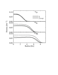
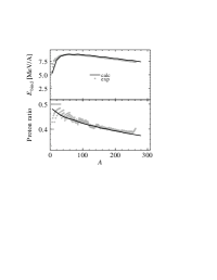
Figure 1: Properties of finite nuclei obtained with the present RMF model. Left: the density profiles of typical nuclei. The proton number densities (solid curves) are compared with the experiment. Right: binding energy per nucleon and the proton number ratio of finite nuclei.

In Fig. 1 (left panel) we show the density profiles of some typical nuclei. One can see how well our framework may reproduce the density profiles. To get a still better fit, especially around the surface region, we might need to include the derivative terms of the nucleon densities, as we have already remarked. Fine structures seen in the empirical density profiles, which may come from the shell effects (see, e.g., a proton density dip at the center of a light ¹⁶O nucleus), cannot be reproduced by the mean-field theory. The effect is seen of the rearrangement of the proton density distribution in heavy nuclei. Protons repel each other, which enhances their contamination near the surface of heavy nuclei. This effect is analogous to the charge screening effect for the Coulomb potential in a sense that the proton distribution is now changed not on the scale of the nuclear radius, but on another length scale, that we will call the proton Debye screening length, see Eq. (16) below. It gives rise to important consequences for the pasta structures since typically the proton Debye screening length is less than the droplet size. The optimal value of the proton ($Z$) to the total baryon ($A$) number ratio $Y_{p}=Z/A$ is obtained by imposing the beta equilibrium condition for a given baryon number. Figure 1 (right panel) shows the baryon number dependencies of the binding energy per baryon and the proton number ratio. We can see that the bulk properties of finite nuclei (density, binding energy, and proton to baryon number ratio) are satisfactorily reproduced for our present purpose.

Note that in our framework we must use a sigma mass $m_{\sigma}=400$ MeV centelles93 , a slightly smaller value than that one usually uses, to get an appropriate fit. If we used a popular value $m_{\sigma}\approx 500$ MeV, finite nuclei would be over-bound by about 3 MeV/$A$. The actual value of the sigma mass (as well as the omega and rho masses) has little relevance for the case of infinite nucleon matter, since it enters the thermodynamic potential only in the combination $\widetilde{C}_{\sigma}=g_{\sigma N}/m_{\sigma}$. However meson masses are important characteristics of finite nuclei and of other non-uniform nucleon systems, like those in pasta. The effective meson mass characterizes the typical scale for the spatial change of the meson field and consequently it affects the value of the effective surface tension voskresurf .

IV Non-uniform structures in nucleon matter

IV.1 Nucleon matter at fixed proton number ratios

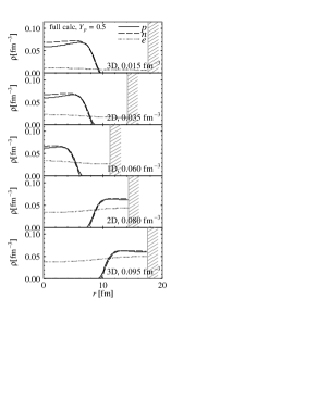
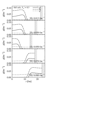
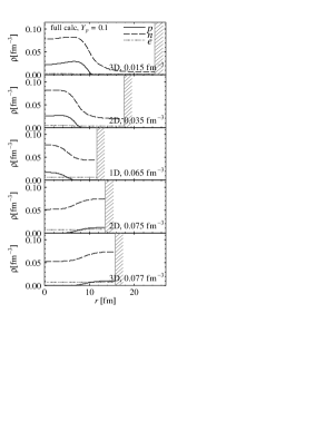
Figure 2: Examples of the density profiles in the cell for symmetric nuclear matter with $Y_{p}$=0.5 (left panel) and for asymmetric matter with $Y_{p}=0.3$ (center panel) and 0.1 (right panel).

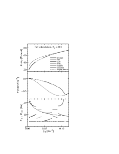
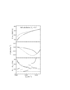
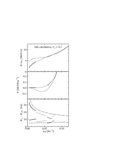
Figure 3: Binding energy per nucleon, baryon partial pressure, and the cell and nuclear sizes for symmetric nuclear matter with $Y_{p}$=0.5 (left panel), and for asymmetric matter with $Y_{p}=0.3$ (center panel) and 0.1 (right panel).

First, we are concentrated on the discussion of the behavior of the nucleon matter at a fixed value of the proton number ratio $Y_{p}$. Particularly, we explore the proton number ratios $Y_{p}=0.1$, 0.3, and 0.5. The cases $Y_{p}=0.3$ – 0.5 should be relevant for the supernova matter and for newly born neutron stars. Figure 2 shows some typical density profiles inside the Wigner-Seitz cells. The geometrical dimension of the cell is denoted as “3D” (three-dimensional sphere), etc. The horizontal axis in each panel denotes the radial distance from the center of the cell. The cell boundary is indicated by the hatch. From the top to the bottom the configuration corresponds to droplet (3D), rod (2D), slab (1D), tube (2D), and bubble (3D). The nuclear “pasta” structures are clearly manifested. For the lowest $Y_{p}$ case ($Y_{p}=0.1$), the neutron density is finite at any point: the space is filled by dripped neutrons; the neutron-drip value of $Y_{p}$ is, e.g., around 0.26 in our 3D calculation. For a higher $Y_{p}$, the neutron density drops to zero outside the nucleus. The proton number density always drops to zero outside the nucleus. We can see that the charge screening effects are pronounced. Due to the spatial rearrangement of electrons the electron density profile becomes no more uniform. This non-uniformity of the electron distribution is more pronounced for a higher $Y_{p}$ and a higher density. Protons repel each other. Thereby the proton density profile substantially deviates from the step-function. The proton number is enhanced near the surface of the nucleus.

The equation of state (EOS) for the sequence of geometric structures is shown in Fig. 3 (top panels) as a function of the averaged baryon-number density. Note that the energy $E-m_{N}$ also includes the kinetic energy of electrons, which makes the total pressure positive. The lowest-energy configurations are selected among various geometrical structures. The most favorable configuration changes from the droplet to rod, slab, tube, bubble, and to the uniform one (the dotted thin curve) with an increase of density. The appearance of non-uniform structures in matter results in a softening of EOS: the energy per baryon gets lower up to about 15 MeV$/A$ compared to the uniform matter.

The middle panels in Fig. 3 are partial pressures without electron contribution versus averaged baryon number density. If electron partial pressure is included, the total pressure becomes positive at all densities.

The bottom panels in Fig. 3 are the cell radii $R_{\rm cell}$ and nuclear radii $R_{d}$ versus averaged baryon number density. The radius $R_{d}$ is defined by way of a density fluctuation as

$$R_{d} = \cases{\displaystyle R_{\rm cell}{\langle\rho_{p}\rangle^{2}\over\langle\rho_{p}^{2}\rangle},\ \ \ \hbox{(for droplet, rod, and slab)}\cr\displaystyle R_{\rm cell}\left(1-{\langle\rho_{p}\rangle^{2}\over\langle\rho_{p}^{2}\rangle}\right),\ \ \ \hbox{(for tube and bubble)}}$$ (15)

where the bracket “$\langle\rangle$” indicates the average along the radial (for 3D and 2D cases) or perpendicular (1D) direction in the cell. Dashed curves show the Debye screening lengths of electron and proton calculated as

$$\lambda^{(e)}_{D} = \left(-4\pi e^{2}{d\rho_{e}^{\rm av}\over d\mu_{e}}\right)^{-1/2},$$ (16)

$$\lambda^{(p)}_{D} = \left(4\pi e^{2}{d\rho_{p}^{\rm av}\over d\mu_{p}}\right)^{-1/2},$$ (17)

where $\rho_{p}^{\rm av}$ is the proton number density averaged inside the nucleus (the region with finite $\rho_{p}$) and $\rho_{e}^{\rm av}$ is the electron charge density averaged inside the cell. Actually doing more carefully we should introduce four Debye screening lengths $\lambda^{(i,<)}_{D}$ and $\lambda^{(i,>)}_{D}$ with a separate averaging for the interior and the exterior of the nuclei. However we observe that the proton number density is always zero in the exterior region and $\lambda^{(p,>)}_{D}=\infty$ thereby. For electrons $\lambda^{(e,<)}_{D}$ and $\lambda^{(e,>)}_{D}$ are in general different but both being large and of the same order of magnitude in the pasta case under consideration. Therefore we actually do not need a more detailed analysis of these quantities. Note that these values are obviously gauge invariant. Numerically, the cell radii $R_{\rm cell}$ for droplet, rod, and slab configurations at $Y_{p}=0.5$ and 0.3 were proven to be close to the electron screening length. For the tube, $R_{\rm cell}$ is larger than ${\lambda}^{(e)}_{D}$. For $Y_{p}=0.1$, in all cases $R_{\rm cell}$ is substantially smaller than ${\lambda}^{(e)}_{D}$ and the electron screening should be much weaker, thereby. In all cases, except for bubbles (at $Y_{p}=0.5$ and 0.3), the structure radii $R_{d}$ are smaller than ${\lambda}_{D}^{(e)}$. This means that the Debye screening effect of electrons inside these structures should not be pronounced. For bubbles at $Y_{p}=0.5$ and 0.3, ${\lambda}_{D}^{(e)}$ is substantially smaller than the cell size and the electron screening should be significant, see Fig. 9 below. For $Y_{p}=0.5$, 0.3, 0.1 in all cases (with the only exception $Y_{p}=0.1$ for slabs), the value ${\lambda}_{D}^{(p,<)}$ is shorter than $R_{d}$. Hence the density rearrangement of protons is essential for the pasta structures, as it is indeed seen from the Fig. 2.

Knowing the baryon number density and the nuclear radius from Fig. 3, one may estimate the atomic number of the nucleus. In the case of droplets and for $Y_{p}=0.5$ the atomic number of the droplet is $\simeq 25$ in the low density limit and $\simeq 65$ at the maximum density of the droplet phase $\rho_{B,d}^{(\rm max)}\simeq 0.025\ {\rm fm}^{-3}$.

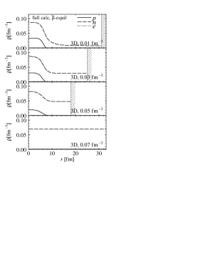
Figure 4: Density profiles in the cell for nuclear matter in beta equilibrium with baryon-number densities, 0.01, 0.03, 0.05 and 0.07 fm^-3 from top to bottom.

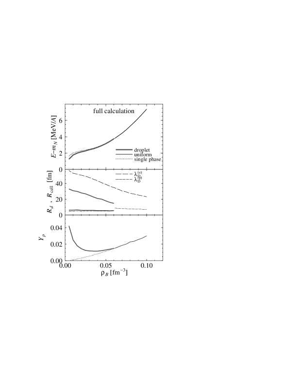
Figure 5: Binding energy (top), cell and nuclear sizes (middle), and proton number ratio (bottom) in the cell for nuclear matter in beta equilibrium.

IV.2 Nucleon matter in beta equilibrium

Next, we consider the neutron star matter at zero temperature, and explore the non-uniform structures for the nucleon matter in beta equilibrium. Figure 5 shows the density profiles for different baryon number densities. The droplet structure itself is quite similar to the case of the fixed proton number ratio $Y_{p}=0.1$ considered above. The apparently different feature in this case is that only the droplet configuration appears as a non-uniform structure. It should be noticed, however, that the presence or absence of the concrete pasta structure sensitively depends on the choice of the effective interaction.

In Fig. 5 we plot the energy per baryon (top), the cell and nuclear sizes (middle), and the proton number ratio (bottom). The effect of the non-uniform structure on EOS (the difference between the energy of uniform matter and that of non-uniform one) is small. However, the proton number ratio is significantly affected by the presence of the pasta at lower densities. In the zero-density limit, the proton number ratio should converge to that of the normal nuclei. The droplet radius and the cell radius in the middle panel of Fig. 5 are always smaller than the electron Debye screening length $\lambda_{D}^{(e)}$. Thereby the effect of the electron charge screening is small. Unlike the fixed $Y_{p}$ cases, the droplet radius is comparable to the proton Debye screening length, which means that the effect of the proton rearrangement is not pronounced in this case. In fact, there is no enhancement of the proton number density near the surface in Fig. 5, in contrast to Fig. 2.

V Comparison with other calculations

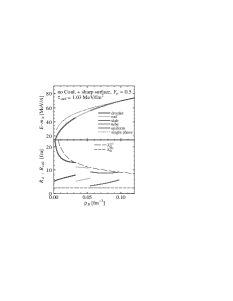
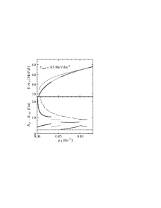
Figure 6: Bulk calculations with the surface tension parameter $\tau_{\rm surf}=1.03$ and 0.5 MeV/fm².

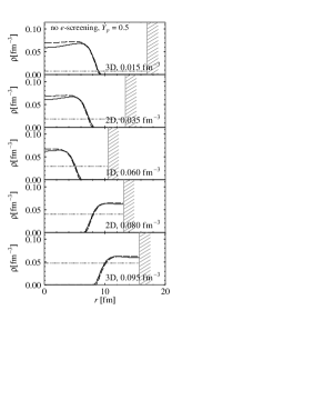
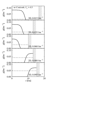
Figure 7: Comparison of the density profiles for different treatments of the Coulomb interaction. From the left: full calculation, without electron screening, and “no Coulomb” calculation. The proton number ratio is $Y_{p}$=0.5 for all cases.

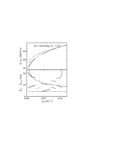
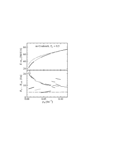
Figure 8: Comparison of the density profiles for different treatments of the Coulomb interaction. From the left: “full” calculation, “no electron screening”, and “no Coulomb” calculation. The proton number ratio is $Y_{p}$=0.5 for all cases.

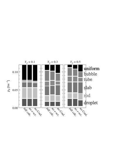
Figure 9: Comparison of the phase diagrams between different treatments of the Coulomb interaction.

In this section we compare our DFT calculation with others to explore the effects of the surface, the charge rearrangement, and the fully consistent treatment of the density distribution.

First let us focus on a very simplified treatment that has been used in the literature. We consider the bulk calculation supplemented by a simplified treatment of the finite-size effect. For description of the latter we introduce the surface tension and a bare (non screened) Coulomb interaction. This calculation assumes a sharp boundary between dense and dilute phases, uniform baryon density distribution inside each phase, and uniform electron density distribution all over the cell. To further specify this approximation we use the term “no Coulomb + sharp surface”. We totally discard the Coulomb potential in equations of motion and drop the Poisson equation (“no Coulomb”) and we reduce the mean fields to their constant bulk values in the interior and the exterior of the structure (“+ sharp surface”). The Coulomb energy, being evaluated with the step-function-like density profiles, and the surface energy, being expressed via the surface tension parameter $\tau_{\rm surf}$ are added to the total bulk energy.

The volume fraction of each phase is simply calculated without taking into account of the finite-size effect (“bulk calculation”). Details of the “no Coulomb + sharp surface” calculation are presented in Appendix A.

Figure 6 shows the EOS obtained by the “no Coulomb + sharp surface” calculation performed at different values of the surface tension. In this case for $Y_{p}=0.5$, the dilute phase includes no baryon. The value of the surface tension parameter $\tau_{\rm surf}\simeq 1.03$ MeV$/$fm² fits the liquid-drop binding energies of finite nuclei. Note that the appearance or disappearance of the pasta structure essentially depends on the value of the surface tension. With a larger value of the surface tension, the density region of the pasta structure reduces and even some of the structures, e.g. “tube” and “bubble”, disappear. With a smaller value of the surface tension the region of the pasta structure broadens and all kinds of pasta structures appear if we take $\tau_{\rm surf}\leq 0.3$ MeV/fm². However, if we put surface tension zero, the mixed phase reaches up from zero to the saturation density $\rho_{0}$ without any specific geometry. Therefore, from the given example we see that the surface tension plays a crucial role in the appearance of pasta structures. Remember that, in the case under consideration, the pasta structures are realized by a balance of the surface tension and the bare Coulomb interaction, which reads $E_{\rm surf}=2E_{\rm Coul}$, where $E_{\rm surf}$ is the surface energy and $E_{\rm Coul}$ is the bare Coulomb energy. Therefore, the Coulomb interaction is important, as well. Please also note that the surface tension introduced here simulates effects of the spatial changes of the meson mean-fields. In our “full calculation” the latter effects are taken into account explicitly whereas purely “bulk calculations” completely disregard these effects.

Next we compare three kinds of calculations with different treatments of the Coulomb interaction. One is the “full calculation” which we have done here. The second is the calculation that disregards electron screening (“no $e$-screening”): a constraint is used that the electron density should be uniform. In this calculation the Coulomb potential $V_{\rm Coul}$ in Eq. (11) is replaced by a constant $V_{0}=0$,

$${\rho_{e}}=-(\mu_{e}-V_{0})^{3}/3\pi^{2}.$$ (18)

In the full calculation the value of $V_{0}$ is arbitrary, and one can take $V_{0}$ for the sake of convenience, e.g. as $V_{0}=0$, either set it equals the averaged value of $V_{\rm Coul}(r)$ over the cell: recall that $V_{\rm Coul}$ either $\mu_{e}$ alone do not have a physical meaning but only the combination $\mu_{e}-V_{\rm Coul}$ is meaningful due to the gauge invariance, cf. voskre ; voskre1 . However in the case “no $e$-screening” the gauge invariance is violated as it follows from Eq. (10), since we replace $V_{\rm Coul}$ to $V_{0}=0$ in the equation for the electron chemical potential but remain $V_{\rm Coul}$ in the equation for the proton chemical potential and thus in the expression for the proton number density. We do this procedure just to demonstrate the efficiency of the proton rearrangement artificially suppressing that of the electron one. The third calculation “no Coulomb” is performed by totally discarding the Coulomb potential $V_{\rm Coul}$ in equations of motion. Accordingly, the Poisson equation is discarded as well. After getting the density profiles, the Coulomb energy, being evaluated using charge densities thus determined, is added to the total energy. This calculation is similar to the above discussed “no Coulomb + sharp surface” calculation. The difference is that the effect of the density variation near the structure surface is automatically incorporated in explicit “no Coulomb” calculation, while in the above “no Coulomb + sharp surface” calculation this effect is hidden in the value of the surface tension.

In Fig. 7 compared are the density profiles for different treatments of the Coulomb interaction. The left panel is the same as that in Fig. 2. It demonstrates the “full” calculation. It seems that there is almost no difference between the nucleon density of the “full” calculation and that of “no $e$-screening” calculation (center). The case of “no Coulomb” calculation (right), contrarily, shows a significant difference especially in the proton number density. The reason is simple: the electron Debye screening length is large, whereas the proton Debye screening length is rather short. Thus the proton screening effects are much more pronounced than the electron ones.

The EOS as a whole (upper panels in Fig. 8) shows almost no dependence on the treatments of the Coulomb interaction. This agrees with a general statement that the variational functional is always less sensitive to the choice of the trial functions than the quantities linearly depending on them. Nevertheless, sizes of the cell and the nucleus (lower panels in Fig. 8) especially for tube and bubbles are different. In the cases of the “full calculation” and “no $e$-screening”, the cell radii of “tube” and “bubble” structures and that of “slab” structure get larger with an increase of density, while they are monotonically decreasing in the case of “no Coulomb” calculation. We see almost no differences between the “full” and “no $e$-screening” calculations that again demonstrates relevance of the proton screening and weakness of the electron screening effects. The only significant difference remains for bubbles as seen from Fig. 9. The other effect illustrated by Fig. 9 is a difference in the density range for each pasta structure. The “full” treatment of the Coulomb interaction slightly increases the region of the nuclear pasta. For $Y_{p}=0.1$ the differences between “full” and “no $e$-screening” calculations are completely washed out.

VI Summary and concluding remarks

We have discussed the low-density nuclear matter structures, “nuclear pasta”, and elucidated the charge screening effect. Using a self-consistent framework based on density functional theory and relativistic mean fields, we took into account the Coulomb interaction in a proper way and numerically solved the coupled equations of motion to extract the density profiles of nucleons.

First we have checked how realistic our framework is by calculating the bulk properties of finite nuclei, as well as the saturation properties of nuclear matter, and found that it can describe both features satisfactorily. One could still improve the consideration fitting other experimental data. For example, we could more carefully fit different terms in the Weiczecker equation like the surface energy and the shell terms. For that we might be need an improvement of our relativistic mean field model that does not include the gradient proton and neutron density terms.

In isospin-asymmetric nuclear matter for fixed proton to baryon number ratios, we have observed the “nuclear pasta” structures with various geometries at sub-nuclear densities. These cases are relevant for the discussion of the supernova explosions and for the description of the newly born neutron stars. The appearance of the pasta structures significantly lowers the energy, i.e. softens the equation of state, while the energy differences between various geometrical structures are rather small. The spatial rearrangement of the proton and electron charge densities (screening) affect the geometrical structures.

By comparing different treatments of the Coulomb interaction, we have seen that the self-consistent inclusion of the Coulomb interaction changes the phase diagram. In particular the region of the pasta structure is broader for “full calculation” compared to that with simplified treatments of the Coulomb interaction which have been used in the previous studies. The effect of the rearrangement of the proton distributions on the structures is much more pronounced compared to the effect of the electron charge screening. The influence of the charge screening on the equation of state, on the other hand, was found to be small.

We have also studied the structure of the nucleon matter in the beta equilibrium. We have found that only one type of structures is realized: proton-enriched droplets embedded in the neutron sea. No other geometrical structures like rod, slab, etc. appeared.

In application to the newly formed neutron stars like in supernova explosions, finite temperature and neutrino trapping effects become important, as well as the dynamics of the first order phase transition with formation of the structures. It would be interesting to extend our framework to include these effects.

This work is partially supported by the Grant-in-Aid for the 21st Century COE “Center for the Diversity and Universality in Physics ” from the Ministry of Education, Culture, Sports, Science and Technology of Japan. It is also partially supported by the Japanese Grant-in-Aid for Scientific Research Fund of the Ministry of Education, Culture, Sports, Science and Technology (13640282, 16540246). The work of D.N.V. was also supported in part by the Deutsche Forschungsgemeinschaft (DFG project 436 RUS 113/558/0-2).

Appendix A “Bulk” and “no Coulomb + sharp surface” calculation of low density nucleon matter

The bulk calculation proceeds like this HPS93 ; pei95 ; GS99 ; ARRW ; Rav83 : first consider two semi-infinite matters, (I) dense and (II) dilute phases, with a sharp boundary. The Coulomb and surface interactions are discarded for a while. Conditions of thermal equilibrium at zero temperature are imposed for pressure $P$ and chemical potential $\mu_{a}$ ($a=n,p$) between two phases:

$$P^{\rm(I)} = P^{\rm(II)},$$

$$\mu_{p}^{\rm(I)} = \mu_{p}^{\rm(II)},$$

$$\mu_{n}^{\rm(I)} = \mu_{n}^{\rm(II)}.$$

In Sec. IV.1 the case is considered when the beta equilibrium is not imposed but the proton to baryon number ratio $Y_{p}$ is fixed.

The averaged densities are $\rho_{p}=f\rho_{p}^{(\rm I)}+(1-f)\rho_{p}^{(\rm II)}$ and $\rho_{n}=f\rho_{n}^{(\rm I)}+(1-f)\rho_{n}^{(\rm II)}$. Here $f$ is the volume fraction of the phase (I). The chemical potentials are calculated using the RMF model presented in this paper. Taking into account the above conditions (LABEL:a1), we obtain a set of $\rho_{n}^{\rm(I)}$, $\rho_{n}^{\rm(II)}$, $\rho_{p}^{\rm(I)}$, $\rho_{p}^{\rm(II)}$, $P^{\rm(I)}=P^{\rm(II)}$, $f$, and the bulk energy density $\epsilon_{\rm bulk}$ in each phase for given $\rho_{n}$ and $\rho_{p}$. At this point $\epsilon_{\rm bulk}$ does not include the surface and Coulomb contributions. If one cannot find the solution with finite $\rho_{n}^{\rm(II)}$ and $\rho_{p}^{\rm(II)}$, the proton or neutron density of the dilute phase is set to be zero. In this case the corresponding chemical potential is larger in the phase (II) than in the phase (I), and the complete set of the Gibbs conditions is not fulfilled. We leave off here the discussion of the “bulk calculation”.

Now let us specify the “no Coulomb + sharp surface” calculation. To consider the structure of the mixed phase, the balance between the Coulomb interaction and the surface one should be taken into account. Introducing an adjusting parameter of the surface tension $\tau_{\rm surf}$, we calculate the surface energy density for the given geometrical dimension $D$:

$$\epsilon_{\rm surf} = {\tau_{\rm surf}fD\over R_{d}},$$ (20)

where $R_{d}$ is the droplet radius. The Coulomb energy density can be calculated Rav83 as

$$\epsilon_{\rm Coul}=2\pi e^{2}\left(\rho_{p}^{\rm(I)}-\rho_{p}^{\rm(II)}\right)^{2}{R_{d}}^{2}f\Phi,$$ (21)

$$\Phi\equiv\left[{2-Df^{1-2/D}\over D-2}+f\right]{1\over D+2}.$$ (22)

By minimization of $\epsilon_{\rm surf}+\epsilon_{\rm Coul}$ in $R_{d}$ (the relation $\epsilon_{\rm surf}=2\epsilon_{\rm Coul}$), we get

$$R_{d} = \left({\tau_{\rm surf}D\over 4\pi\left(\rho_{p}^{\rm(I)}-\rho_{p}^{\rm(II)}\right)^{2}\Phi}\right)^{1/3},$$ (23)

$$\epsilon_{\rm Coul}+\epsilon_{\rm surf} = 3fD\left({\pi\tau_{\rm surf}^{2}\left(\rho_{p}^{\rm(I)}-\rho_{p}^{\rm(II)}\right)^{2}\Phi\over 2D}\right)^{1/3}.$$ (24)

Comparing the energy density of the uniform matter $\epsilon$ and those of mixed phases $\epsilon_{\rm bulk}+\epsilon_{\rm surf}+\epsilon_{\rm Coul}$ with different geometrical dimension $D$, we can determine the most favorable configuration and its energy density.

References

- (1) N. K. Glendenning, Phys. Rev. D46, 1274 (1992); N. K. Glendenning, Phys. Rep. 342, 393 (2001).
- (2) H. Heiselberg, C. J. Pethick and E. F. Staubo, Phys. Rev. Lett. 70, 1355 (1993).
- (3) N. K. Glendenning and S. Pei, Phys. Rev. C D52, 2250 (1995).
- (4) D. N. Voskresensky, M. Yasuhira and T. Tatsumi, Phys. Lett. B541, 93 (2002); T. Tatsumi and D. N. Voskresensky, nucl-th/0312114.
- (5) D. N. Voskresensky, M. Yasuhira and T. Tatsumi, Nucl. Phys. A723, 291 (2003).
- (6) T. Endo, Toshiki Maruyama, S. Chiba and T. Tatsumi, nucl-th/0410102; hep-ph/0502216.
- (7) N. K. Glendenning and J. Schaffner-Bielich, Phys. Rev. C60, 025803 (1999).
- (8) M. B. Christiansen and N. K. Glendenning, astro-ph/0008207.
- (9) M. Christiansen, N. K. Glendenning and J. Schaffner-Bielich, Phys. Rev. C62, 025804 (2000).
- (10) J. A. Pons, S. Reddy, P. J. Ellis, M. Prakash and J. M. Lattimer, Phys. Rev. C62, 035803 (2000).
- (11) M. Yasuhira and T. Tatsumi, Nucl. Phys. A690, 769 (2001).
- (12) S. Reddy, G. Bertsch and M. Prakash, Phys. Lett. B475, 1 (2000).
- (13) T. Norsen and S. Reddy, Phys. Rev. C63, 065804 (2001).
- (14) Toshiki Maruyama, T. Tatsumi, D. N. Voskresensky, T. Tanigawa and S. Chiba, Nucl. Phys. A749, 186 (2005).
- (15) T. Tatsumi, Toshiki Maruyama, D. N. Voskresensky, T. Tanigawa and S. Chiba, nucl-th/0502040.
- (16) M. Alford, K. Rajagopal, S. Reddy and F. Wilczek, Phys. Rev. D64, 074017 (2001).
- (17) P. F. Bedaque, Nucl. Phys. A697, 569 (2002).
- (18) S. Reddy and G. Rupak, nucl-th/0405054.
- (19) P. F. Bedaque, H. Caldas and G. Rupak, Phys. Rev. Lett. 91, 247002 (2003).
- (20) D. G. Ravenhall, C. J. Pethick and J. R. Wilson, Phys. Rev. Lett. 50, 2066 (1983).
- (21) M. Hashimoto, H. Seki and M. Yamada, Prog. Theor. Phys. 71, 320 (1984).
- (22) R. D. Williams and S. E. Koonin, Nucl. Phys. A435, 844 (1985).
- (23) K. Oyamatsu, Nucl. Phys. A561, 431 (1993).
- (24) C. P. Lorenz, D. G. Ravenhall and C. J. Pethick, Phys. Rev. Lett. 70, 379 (1993).
- (25) K. S. Cheng, C. C. Yao and Z. G. Dai, Phys. Rev. C55, 2092 (1997).
- (26) Toshiki Maruyama, K. Niita, K. Oyamatsu, Tomoyuki Maruyama, S. Chiba and A. Iwamoto, Phys. Rev. C57, 655 (1998).
- (27) T. Kido, Toshiki Maruyama, K. Niita and S. Chiba, Nucl. Phys. A663-664, 877 (2000).
- (28) G. Watanabe, K. Iida and K. Sato, Nucl. Phys. A676, 445 (2000);
- (29) G. Watanabe, K. Sato, K. Yasuoka and T. Ebisuzaki, Phys. Rev. C66, 012801(R) (2002).
- (30) G. Watanabe and K. Iida, Phys. Rev. C68, 045801 (2003).
- (31) C. J. Horowitz, M. A. Pérez-García, and J. Piekarewicz, Phys. Rev. C69, 045804 (2004).
- (32) Y. Mochizuki and T. Izuyama, Astrophys. J. 440, 263 (1995).
- (33) Toshiki Maruyama, T. Tatsumi, D. N. Voskresensky, T. Tanigawa, S. Chiba and Tomoyuki Maruyama, nucl-th/0402202.
- (34) Density Functional Theory, ed. E. K. U. Gross and R. M. Dreizler, Plenum Press (1995).
- (35) D. N. Voskresensky et al., in preparation.
- (36) M. Centelles and X. Viñas, Nucl. Phys. A563, 173 (1993).