Particle yield fluctuations and chemical non-equilibrium at RHIC

Abstract

We study charge fluctuations within the statistical hadronization model. Considering both the particle yield ratios and the charge fluctuations we show that it is possible to differentiate between chemical equilibrium and non-equilibrium freeze-out conditions. As an example of the procedure we show quantitatively how the relative yield ratio $\Lambda/K^{-}$ together with the normalized net charge fluctuation $v(Q)=\left\langle\Delta Q^{2}\right\rangle/\left\langle N_{\rm ch}\right\rangle$ constrain the chemical conditions at freeze-out. We also discuss the influence of the limited detector acceptance on fluctuation measurements, and show how this can be accounted for within a quantitative analysis.

I introduction

In relativistic heavy ion collisions a localized high energy density domain, a fireball, is created. The study of the properties of this hot and dense matter is the main objective of the experiments being conducted at RHIC and as of 2007 at LHC. Event-by-event particle fluctuations are the observables subject to intense current theoretical fluct1 ; fluct2 ; fluct3 ; fluct4 ; fluct4b ; fluct5 ; fluct6 ; fluct7 ; fluct8 , and experimental  starfluct ; starfluct2 ; phefluct interest. Fluctuation measurements are important since they can be used: (i) as a consistency check for existing models, e.g. within statistical particle production models fluct2 ; fluct3 , (ii) as a way to search for new physics, including QGP fluct4 ; interm2 ; interm3 (iii) as a test of particle equilibration fluct2 ; fluct8 .

The statistical hadronization model (SHM), introduced by Fermi in 1950 Fer50 ; Pom51 ; Lan53 , has been used extensively in recent years in the study of strongly interacting particle production. In this model, the properties of the final state particles are determined by requiring that the final state maximizes entropy given the physical properties of the fireball (energy, baryon content, etc.). When the full spectrum of hadronic resonances is included Hag65 , the SHM turns into a quantitative model capable of describing in detail the abundances of all hadronic particles.

Fluctuations in conserved quantum numbers (such as charge, baryon number, strangeness, or equivalently the net multiplicities of up, down and strange quarks) can be studied only in the Grand Canonical (GC) ensemble, since in the micro-canonical and canonical ensembles these quantities are fixed. We also mention here that fluctuations of non-conserved observables, e.g. other hadron multiplicities, differ for different ensembles even in the thermodynamic limit nogc1 ; nogc2 .

In this paper we will discuss the use of fluctuations as a phenomenological tool within the framework of the statistical model, and illustrate some issues pertinent in analyzing fluctuations data. In section II we will motivate the choice of charge fluctuations as a useful experimental probe. After demonstrating, in section III, how the statistical model implies a scaling between fluctuations and yields, we show (section IV) that a measurement of both particle yields and charge fluctuations can distinguish between an equilibrium high temperature statistical freeze-out from a super-cooled over-saturated freeze-out from a high entropy phase. Finally, in section V we discuss issues related to detector acceptance which impact the fluctuation measurement even in a boost-invariant azimuthally symmetric limit. We quantitatively demonstrate how such limited acceptance effects can be taken into account and the freeze-out temperature and non-equilibrium parameters extracted from experimental data.

II GC Observables

A study of GC SHM fluctuations of conserved quantities is of considerable interest at RHIC. Since the detectors at RHIC (except for the PHOBOS detector) only see small portions of the final phase space, using the grand-canonical approach is justified in the following sense: Provided the fireball is indeed locally thermalized, we can take the experimentally observed source to be a subsystem in contact with a larger reservoir.

The situation is of particular interest for reactions at RHIC that exhibit a sizable central plateau in the (pseudo-)rapidity spectrum, since a limited (pseudo)rapidity acceptance window selects a suitable subset of the source particles. Specifically, it can be shown (sections cleymans . The reasoning used there can be generalized to Fermi-Dirac and Bose-Einstein statistics) that the rapidity spectrum of a boost invariant system could be related to the multiplicity in a static GC system with the same temperature and chemical potentials

$${\left\langle dN_{i}/dy\right\rangle_{\rm b.i.}\over\left\langle dN_{j}/dy\right\rangle_{\rm b.i.}}={\left\langle N_{i}\right\rangle_{\rm GC}\over\left\langle N_{j}\right\rangle_{\rm GC}}$$ (1)

where $i$ and $j$ are species labels and the subscripts ${\rm b.i.}$ and ${\rm GC}$ denote the boost invariant system and the grand canonical system, respectively.

The derivation in cleymans can be applied to fluctuations at hadronization (before resonance decays) to show

$${\left\langle d{\Delta N_{i}^{2}}/dy\right\rangle_{\rm b.i.}\over\left\langle dN_{j}/dy\right\rangle_{\rm b.i.}}={\left\langle\Delta N_{i}^{2}\right\rangle_{\rm GC}\over\left\langle N_{j}\right\rangle_{\rm GC}}$$ (2)

where we denote the variance (fluctuation) of any quantity $X$ as $\left\langle\Delta X^{2}\right\rangle=\left\langle X^{2}\right\rangle{-}\left\langle X\right\rangle^{2}$.

Given this, SHM average yields and yield fluctuations can be calculated by a textbook method huang , as per section III.

When studying finite systems the consideration of fluctuations in extensive quantities such as of particle yield has to address also volume fluctuations when the volume cannot be fixed by experimental conditions. In our case volume fluctuations can arise due to initial reaction effects, impact parameter variations, as well as from fluctuations due to dynamics of the expanding fireball. It is difficult to arrive at a reliable description of all these effects. Therefore it is important to select fluctuation observables in which volume fluctuation effects are sub-dominant. Among extensive quantities, the net charge fluctuation stands out as it is relatively easy to measure and can be shown to be nearly independent of the volume fluctuations fluct1 .

In light of the above considerations we concentrate our effort on the following net charge fluctuation measure:

$$v(Q)\equiv\left<\Delta Q^{2}\right>/\left<N_{\rm ch}\right>$$ (3)

(where $N_{\rm ch}=N_{+}+N_{-}$) proposed in the past as a probe of the QGP formation fluct4 . First results for $v(Q)$ are also available from RHIC experiments starfluct2 ; phefluct .

In the SHM, the charged particle multiplicity is given by summing all final state (stable) charged particle multiplicities. These can be computed by adding the direct yield and all resonance decay feed-downs. The total yield of a stable particle $\alpha$ is

$$\langle N_{\alpha}\rangle_{\rm total} = \langle N_{\alpha}\rangle_{\rm GC}+\sum_{j\neq\alpha}B_{j\rightarrow\alpha}\langle N_{j}\rangle_{\rm GC}$$ (4)

where $j$ labels resonances. $B_{j\rightarrow\alpha}$ is the probability (branching ratio) for the decay products of $j$ to include $\alpha$. The charged particle multiplicity is given by the sum of all charged stable particles.

The net charge fluctuation is given by

$$\left\langle\Delta Q^{2}\right\rangle_{\rm GC}=\sum_{i}q_{i}^{2}\left\langle\Delta N_{i}^{2}\right\rangle_{\rm GC}$$ (5)

where $q_{i}$ is the particle charge and $i$ labels all particles before resonance decays since net charge is conserved fluct3 .

To use Eq.(5) quantitatively, however, the experimental rapidity window must be large enough to encompass all decay particles of the resonances, yet small enough for the GC ensemble to maintain it’s validity. See section V for a discussion of the validity of this assumption, and how to incorporate deviations from it in realistic experimental situations.

III Statistical hadronization

For a hadron with an energy $E_{p}=\sqrt{p^{2}+m^{2}}$, the GC partition function for each species is given by

$$\ln Z_{i}=(\mp)Vg_{i}\int{d^{3}p\over(2\pi)^{3}}\ln\left(1\pm\lambda_{i}e^{-E_{i}/T}\right)$$ (6)

where $g_{i}$ is the degeneracy factor and the upper sign is for bosons and the lower sign is for fermions. Here $\lambda_{i}$ is the particle fugacity, related to particle chemical potential $\mu_{i}=T\ln\lambda_{i}$.

The yield average and fluctuation is then given by:

$$\langle N_{i}\rangle_{\rm GC} = \frac{\partial\ln Z_{i}}{\partial\lambda_{i}}=g_{i}V\int{4\pi p^{2}dp\over(2\pi)^{3}}\,n_{i}(E_{p}),$$ (7)

$$\left\langle\Delta N_{i}^{2}\right\rangle_{\rm GC} = \frac{\partial^{2}\ln Z_{i}}{\partial\lambda_{i}^{2}}$$ (8)

$$= g_{i}V\int{4\pi p^{2}dp\over(2\pi)^{3}}\,n_{i}(E_{p})\left(1\mp n_{i}(E_{p})\right).$$

and

$$n_{i}(E_{p})={1\over\lambda_{i}^{-1}e^{E_{p}\beta}\pm 1},$$ (9)

We note that $\lambda_{i}$ enters the partition function in Eq.(6). Hence, the validity of Eqs.(7) and (8) depends on weather Eq.(6) can be used as a generating function for the probability distribution of states. It is important to underline this as in a dynamical system the value of $\lambda_{i}$ is not determined solely in terms of entropy maximization, but is subject to chemical conditions prevailing in the system, and here importantly, includes effects related to chemical non-equilibrium. Where Eq. 6 represents a generating function but the system is not in chemical equilibrium, the fugacity $\lambda_{i}$, is not anymore a Lagrange multiplier but a parameter characterizing the quantum number density.

In a scenario where freeze-out occurs as a break-up of a chemically equilibrated hadron gas, the fugacity of the hadron $i$ is given by the product of the fugacities of conserved quantum numbers.

$$\lambda_{i}^{\mathrm{eq}}=\lambda_{q}^{q-\overline{q}}\lambda_{s}^{s-\overline{s}}\lambda_{I_{3}}^{I_{3}}\;,\;\lambda_{\overline{i}}^{\mathrm{eq}}=(\lambda_{i}^{\mathrm{eq}})^{-1},$$ (10)

where $\overline{q},q$ is the number of light anti-quarks and quarks, respectively and $\overline{s},s$ is the number of strange anti-quarks and quarks, respectively and $I_{3}$ is the isospin. This formula implies that the fugacity for the antiparticle is, in full chemical equilibrium, the inverse of the fugacity for the particle, and the fugacity for a hadron carrying vanishing conserved quantum numbers is 1.

In our approach, we do not assume that that the chemical equilibrium is reached JJBook ; Rafelski:2003ju . Hence Eq.(10) no longer applies. The deviation from chemical equilibrium can be parametrized by a phase space occupancy factor $\gamma_{q}$ (for $u,\bar{u},d,\bar{d}$ in hadrons) and $\gamma_{s}$ (for $s$ and $\bar{s}$). In this chemical nonequilibrium case the fugacity becomes

$$\lambda_{i}=\lambda_{i}^{\mathrm{eq}}\gamma_{q}^{q+\overline{q}}\gamma_{s}^{s+\overline{s}}$$ (11)

where $\lambda_{i}^{\mathrm{eq}}$ is given by Eq.(10) (Note that $\gamma_{i}=\gamma_{\overline{i}}$).

A system undergoing collective expansion is unlikely to be in chemical equilibrium, since collective expansion and cooling will make it impossible for endothermic and exothermic reactions, or for creation and destruction reactions of a rare particle, to be balanced. However, since inelastic collisions have in general a slower relaxation time than elastic ones, an approximately perfect fluid can still have $\gamma\neq 1$ (it’s evolution will be a non-trivial function of time, since $\gamma$ does not commute with the Hamiltonian). Furthermore, light quark chemical nonequilibrium is well motivated in a scenario where an entropy rich deconfined state quickly hadronizes Rafelski:2000by . In this scenario, mismatch of entropies between the two phases requires $\gamma_{q}>1$.

Despite the lack of equilibrium and entropy maximization w.r.t. conserved quantum numbers, we will argue that the Eqs. 8 and 7 apply in such a situation, with $\gamma$ s contributing to the chemical potential via Eq.(11). The validity of Eq.(8) and (7) depend on the extent that Eq.(6) represents a probability generating function for the statistically hadronizing system. Within a statistical hadronization scenario where hadrons are formed in proportion to their phase space weight given (not necessarily equilibrated) densities Danos , this is indeed the case provided the dynamics behind $\gamma$ does not generate additional, non-statistical fluctuations. For an instance where the last issue is a concern, fluctuations of a quantum number produced mostly in initial-state processes (such as charm thews ; becattini_charm ) will likely be dominated not by the statistical hadronization contribution but to fluctuations in initial abundance.

Given that in the considered model non-equilibrium arises due to the rapid hadronization of the collectively expanding system Rafelski:2000by , and since the observable charged particles are produced not in in the initial state but during the final break-up of a locally thermalized system, such non-statistical fluctuations should not be significant for the observable we are considering. Similarly, as we have argued in the previous section, initial-state volume fluctuations give a negligible contribution to the observable under consideration.

However, it is possible that additional sources of irreducible two-particle correlations and fluctuations could arise near a phase transition. These effects go beyond the scope of this work. We will however argue that the applicability of our scenario, and the absence of further correlations can be tested by requiring that the same temperature and $\gamma$ s describe both the yields and the fluctuations of all soft hadronic observables. As we will show, this is a very stringent requirement. If it turns out that a single set of $T$, $\lambda^{\rm eq}$ and $\gamma_{q}$ and $\gamma_{s}$ is capable of describing all yields and fluctuations, then it certainly is a strong indication that Eq.(6) can be interpreted as a generating function of the probabilities. The goal of this paper is then to find a way to experimentally determine the additional parameter $\gamma_{q}$ which can be then used to compare the SHM calculation of yields and fluctuations to the experimental measurements.

IV fluctuations in chemical non-equilibrium

Chemical nonequilibrium is of a particular interest since it can result in a large pion fugacity which influences fluctuations much more severely than the yields.

If $\gamma_{q}$ becomes large enough so that $\lambda_{\pi}$ approaches $e^{m_{\pi}/T}$, then the pion yield and the fluctuations behave like (c.f. Eqs.(7,8))

$$\lim_{\epsilon\rightarrow 0}\langle N\rangle\propto\epsilon^{-1},\qquad\lim_{\epsilon\rightarrow 0}(\Delta N)^{2}\propto\epsilon^{-2}.$$ (12)

where $\epsilon=1-\lambda_{\pi}e^{-m_{\pi}/T}$. The fluctuation grows much faster than the yield as mentioned above.

Some studies of yield ratios have indeed found the value of $\gamma_{q}$ that can potentially make $\epsilon$ small observing ; Rafelski:2003ju ; Rafelski:2004dp ; gammaq_energy . However, other studies of yield ratios Becattini:2003wp concluded that $\gamma_{q}$ is not necessarily large due to the fact parameters in such fits are highly correlated. In this case, adjusting other parameters such as the temperature can accommodate current data without having $\gamma_{q}\neq 1$, but with much reduced statistical significance. Since such conflict is common when only the yields are considered, it becomes necessary to study fluctuations as an additional constraint to determine the occupation factor $\gamma_{q}$ more convincingly.

We now discuss our specific analysis results. We used the public domain SHM suite of programs SHARE share , expanded to include the fluctuations share2 . We evaluate yields and fluctuations, allowing for production of hadron resonances, their decay, and a possible absence of chemical equilibrium. In the rest of this paper, we set $\lambda_{I_{3}}^{\rm eq}=1,\lambda_{q}^{\rm eq}=e^{\mu_{B}/3T}=1.05$ and $\lambda_{s}^{\rm eq}=1.027$ in accordance with Rafelski:2004dp . However, the two observables we consider, the net charge fluctuations and the $\Lambda/{\rm K}^{-}$ particle yield ratio, are nearly independent of these quantities as will be shown below.

Figure 1: (Color online) $v(Q)$ as function of $\gamma_{q}$ (solid lines). Dot-dashed lines, no resonance decays; dashed lines, Boltzmann fluctuations. Ellipses (blue) indicate the expected result areas for the equilibrium ($\gamma_{q}=1$, solid) and non-equilibrium ($\gamma_{q}\neq 1$, dashed) models.

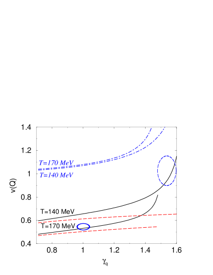
Fig. 1 shows the variation in $v(Q)$ as a function of $\gamma_{q}$ for $T=140,170$ MeV. The solid lines show $v(Q)$ including the resonance decays, dot-dashed lines comprise only the direct effect of pion fluctuations. As the temperature increases (solid lines from top to bottom) the number of resonances increases. This in turn increases the unlike-sign charge correlations and hence reverses the temperature dependence of the pure pion case (dot-dashed lines). The short dashed lines show results for Boltzmann statistics. Boltzmann charge fluctuations are nearly constant as function of $\gamma_{q}$ and primarily depend on chemical mix of the directly produced and secondary decay particles, which dominantly depend on the temperature $T$. The solid and dot-dashed lines in Fig. 1 terminate when the fluctuations start to diverge as in Eq.(12).

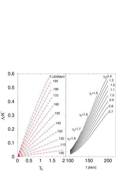
To determine both $T$ and $\gamma_{q}$ values we require an additional observable. In this work, we choose the yield ratio $\Lambda/K^{-}$. This ratio depends linearly on $\gamma_{q}$, and is nearly independent of $\lambda_{s}^{\rm eq}$ and $\gamma_{s}$ as $\Lambda=(sdu)$ and $K^{-}=(s\bar{u})$. In Fig. 2 we show how the relative yield depends on $\gamma_{q}$ and $T$. The $\Lambda$ yield we wish to consider does not include weak decay feed from $\Xi$ but it includes the electromagnetic decay of $\Sigma^{0}$ and the strong decays. $K^{-}$ excludes feed-down from $\phi$, but includes $K^{*}$ and higher resonances. It is important to exclude the $\Xi$ and $\phi$ cascading in order to eliminate the dependence on $\gamma_{s}$ and $\lambda_{s}^{\rm eq}$. Fortunately, this is experimentally feasible.

A similar ratio, which is experimentally easier to correct for, is $\Xi/\phi$, also dependent on temperature and $\gamma_{q}$ only. See ourfluct2 for the equivalent discussion in terms of $\Xi/\phi$.

Figure 2: (Color online) Particle yield ratio $\Lambda/K^{-}$ as a function of $T$ (right panel) and $\gamma_{q}$ (left panel) The $\Lambda$ yield does not include $\Xi\rightarrow\Lambda$ and the ${\rm K^{-}}$ yield is without the contribution of $\phi\rightarrow{\rm K^{+}}{\rm K^{-}}$ decays. Ellipses (blue) indicate the expected result areas for the equilibrium ($\gamma_{q}=1$, solid) and non-equilibrium ($\gamma_{q}\neq 1$, dashed) models.

We now combine results in Figs. 1 and 2 into our main result Fig. 3. Every point in this plane of $v(Q)$ and $\Lambda/K^{-}$ corresponds to a specific set of $T$ and $\gamma_{q}$ as indicated by the grid. Note that some domains in this plane are not allowed since they lie in the region where the (generating, GC) partition function cannot be defined. The two highlighted regions indicate the expected chemical equilibrium (solid line ellipse at small $v(Q)$, corresponding to $\gamma_{q}=1$ and $T=170$ MeV) and nonequilibrium parameter domains (dashed line ellipse at larger $v(Q)$, corresponding to $\gamma_{q}=1.62$ and $T=140$ MeV). When particle yields and fluctuations are considered, the separation of these two domains confirms that we have found a sensitive method to determine both $\gamma_{q}$ and $T$.

Figure 3: (Color online) Particle ratio $\Lambda/K^{-}$ and particle fluctuation $v(Q)$ plane: a point in plane corresponds to a set of values $\gamma_{q},T$. Black Lines correspond to results at fixed $T=200$ (top), 170, 140, 100 MeV (bottom). The red dashed lines are for $\gamma_{q}=0.8,1,1.4,1.6,1.8$ from left to right. Thick lines correspond to $\gamma_{s}=2.5$, thin lines correspond to $\gamma_{s}=1$. Ellipses (blue) indicate the expected result areas for the equilibrium ($\gamma_{q}=1$, solid) and non-equilibrium ($\gamma_{q}\neq 1$, dashed) models.

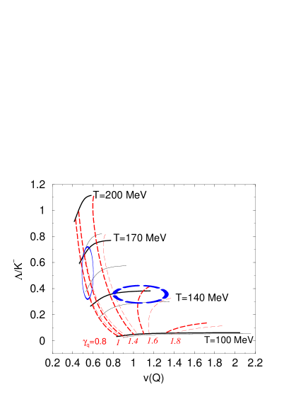
The results of having two extreme values, $\gamma_{s}=1$ and $\gamma_{s}=2.5$, are also shown in Fig. 3. The $\gamma_{s}$ values corresponds to the equilibrium bdm and non-equilibrium Rafelski:2003ju best fits. Their difference, as seen in Fig. 3, is small and well below the experimental error. The largest remaining systematic deviation is due to the baryon chemical potential $e^{\mu_{B}/3T}=\lambda_{q}^{\rm eq}$. It’s contribution to $v(Q)$ is negligible, but this is not true for the case of $\Lambda/K^{-}$. Generally the value of $\lambda_{q}^{\rm eq}$ is well determined by baryon to antibaryon yield ratios in a model independent way.

To transform the diagram in Fig. 3 (or $\Xi/\phi$ in ourfluct2 ) to an equivalent result applicable to lower reaction energy where $\lambda_{q}^{\rm eq}$ is greater, one has to allow for this change: We note that $\Lambda/K^{-}\propto(\lambda_{q}^{\rm eq})^{3}$, and thus we need to multiply the axis in Figs. 2 and 3 by $(\lambda_{q}^{\rm eq})^{3}/1.05^{3}$. One can actually use the $\Lambda/K$ ratio in this. Since ${\Lambda K^{+}}/{\overline{\Lambda}K^{-}}\propto(\lambda_{q}^{\rm eq})^{6}$, the axis rescaling would be done with $({\Lambda K^{+}}/{\overline{\Lambda}K^{-}})^{1/2}/1.05^{3}$ ($\Lambda,K$ corrected for $\Xi$ and $\phi$ feed-down).

V Issues related to detector acceptance

The main phenomenological issue that prevents the straight-forward extraction of parameters from graphs such as Fig. 3 are effects relating to the detector acceptance. First of all, it has long been known that $v(Q)$ is not a “robust” observable, but in general depends on the detector’s kinematic (rapidity and $p_{T}$) cuts. This difficulty, however, can be lessened via mixed event background subtraction. It can be shown fluct6 that observables corrected this way are in certain limits “robust” w.r.t. kinematic cuts and detector response.

We have discussed how to generalize the methods described in this paper to robust observables elsewhere ourfluct1 ; ourfluct2 ; ourfluct3 , and hence will not dwell on this topic, beyond noting that, while diagrams such as Fig. 3 need to be re-thought since dynamical observables generally also depend on the (average) system volume, the sensitivities of the fluctuation and yield observables to the statistical model parameters follow the pattern described by this paper. Hence, generalizing the methods described by this paper to dynamical observables (whether via fits, as was done in ourfluct3 or three-dimensional diagrams), is not a difficult task.

An issue that needs to be addressed separately, however, is the acceptance dependence of particle correlations. If the detector’s pseudo-rapidity coverage is too large, than the small volume assumption required for the Grand-Canonical ensemble becomes untenable, and long-range correlations (such as global conservation laws) can modify fluctuations. If the detector’s pseudo-rapidity coverage is too small, correlations due to resonance decays acquire a rapidity-dependent correction (which is not eliminated by mixed-event subtraction since it corrects two-particle correlations). We will address these issues in the next sub-sections.

V.1 Influence of conservation laws on fluctuations

If the detector can capture the full phase space of the system than, barring dramatic departure from standard model physics, the net charge of the event can not fluctuate. More generally, if the phase space size of the detected system becomes comparable to the total system size, observables will not anymore be given by the Grand-Canonical ensemble.

If the system is a fluid (or in general not in global equilibrium) no ensemble is expected to provide a good description of fluctuations beyond the small volume Grand Canonical limit, since the observable region of phase space will include many locally equilibrated volume elements exchanging energy and quantum numbers via hydrodynamic flow. While yields could still be approximated by some ensemble, the long range correlations and global non-equilibrium should break all simple scaling of fluctuations with yields.

Hence, the configuration space coverage needed for a statistical description needs to be appropriately small for the corrections to the GC ensemble to be kept under control.

To investigate these corrections quantitatively, consider the Taylor-expansion of the entropy of the “reservoir”:

$$S(N_{\rm tot}-N) \approx S(N_{\rm tot})-N\left.\frac{\partial S}{\partial N}\right|_{N_{\rm tot}}$$ (13)

$${}+\frac{1}{2}N^{2}\left.\frac{\partial^{2}S}{\partial N^{2}}\right|_{N_{\rm tot}}+...$$

where $N_{\rm tot}$ is the total number of particles in the reservoir and the small subsystem, and $N$ is the number of particles in the subsystem. The first and second terms result in the usual Grand-Canonical ensemble result huang through the identification of the equilibrium chemical potential $\mu=-T(\partial S/\partial N)$.

The third term gives the first correction; The Grand-Canonical ensemble is therefore a valid approximation when

$$\zeta_{GC}=\frac{\left\langle N\right\rangle}{2}\frac{({\partial^{2}S}/{\partial N^{2}})_{N_{\rm tot}}}{({\partial S}/{\partial N})_{N_{\rm tot}}}\ll 1$$ (14)

This quantity can be easily related to more common thermodynamic quantities

$$\zeta_{GC}=\frac{1}{2}\frac{T\left\langle N\right\rangle}{\mu}{k_{Vtot}}$$ (15)

where $\left\langle N\right\rangle$ is the average multiplicity of the observed volume and $k_{Vtot}$ is the susceptibility of the total volume. For the relativistic ideal gas, this is given by

$$\zeta_{GC}=\frac{V}{2V_{tot}}\ \left[\frac{\sum_{n=0}^{\infty}\lambda^{n}m^{2}TK_{2}\left(\frac{nm}{T}\right)}{\ln\lambda\sum_{n=0}^{\infty}\lambda^{n}m^{2}\frac{T}{n}K_{2}\left(\frac{nm}{T}\right)}\right]$$ (16)

and, as shown in section II

$$\ \frac{V}{V_{tot}}=\frac{\Delta\eta}{(\Delta\eta)_{tot}}$$

where $\Delta\eta$ is the detector’s (pseudo)rapidity coverage and $(\Delta\eta)_{tot}$ is the system’s rapidity interval.

Thus, we discover that the larger the susceptibility is, the smaller the system size $V/V_{\rm tot}$ has to be for the Grand-Canonical limit to hold.

In fact, the physics determining the departure from this limit is precisely the same as the physics determining the divergence of fluctuations within an over-saturated pion gas. This is unsurprising, since over-saturation is argued for as a signature of a phase transition, and in finite systems undergoing phase transitions it is the finite size of the system that gives a cut-off for fluctuations.

The pion chemical potential of the system created at RHIC, however, is kept below divergence, so it is hoped that one unit of rapidity, corresponding to $V/(2V_{\rm tot})\sim 7\%$, provides a safe limit for the Grand Canonical ensemble. In such a small rapidity interval, however, correlations due to resonances need to be suitably accounted for. The next sub-section shows how to do that.

V.2 Disappearance of resonance correlations at small $\Delta\eta$

If charge fluctuations are calculated after all resonances have decayed, then Eq. 5 becomes

$$\left\langle(\Delta Q)^{2}\right\rangle=\left\langle(\Delta N_{+})^{2}\right\rangle+\left\langle(\Delta N_{-})^{2}\right\rangle-2\left\langle\Delta N_{+}\Delta N_{-}\right\rangle$$ (17)

where the last term accounts for unlike-sign charge correlations coming from the decay of neutral resonances. For a conserved charge, and full acceptance of all resonances, this expression is equivalent to Eq.(5), with the correlation term exactly balancing out the amplification of resonance abundance fluctuations through the greater multiplicity of resonance decay products. within a hadron gas the correlation term will be given by decays of the resonance $j$ into $N_{+}$ and $N_{-}$

$$\left\langle\Delta N_{+}\Delta N_{-}\right\rangle=\sum_{j}b_{j\rightarrow+-}\left\langle N_{j}\right\rangle$$ (18)

while the fluctuation of each stable $N_{\pm}$ has to be augmented by contributions to it from resonance decays fluct1

$$\left\langle(\Delta N_{\pm})^{2}\right\rangle = \sum_{i}\left\langle(\Delta N_{\pm})^{2}\right\rangle_{i}+$$

$$+\left(\sum_{j}b_{j\rightarrow i}(1-b_{j\rightarrow i})\left\langle N_{j}\right\rangle+b_{j\rightarrow i}^{2}\left\langle(\Delta N_{j})^{2}\right\rangle\right)$$

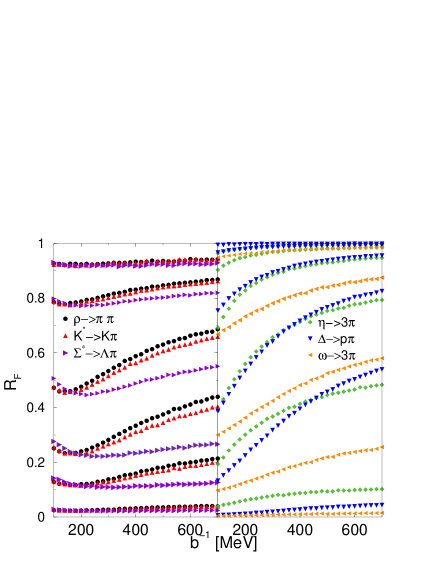
For a finite acceptance window in general not all resonances produced can be reconstructed, even if the efficiency of the detector were 100%. Hence these contributions must be weighted with acceptance weight factors, and this applies here in particular to the limited rapidity acceptance. For a neutral resonance $j$ decaying into $n_{+}$ positive particles and $n_{-}$ negative particles, three such coefficients are needed:

Two will be the fractions of the positively charged and the negatively charged decay products which land in the acceptance window, and the third will give the fraction of the $+-$ pairs that will land in the window. These coefficients will modify the branching ratios $b_{j\rightarrow i}$ in Eq.(V.2) and $b_{j\rightarrow+-}$ in Eq.(18).

If boost-invariance is a good symmetry, the first two coefficients can be fixed to unity, since particles coming out of the acceptance region are exactly balanced by particles coming in. However, this is not true for the number of detectable pairs. If the resonance is out of the detector’s acceptance window it is impossible for all of it’s decay products to be in a window. Hence, Eq.(17) will have to include a term giving the percentage of resonances whose decay products are both within the detector’s acceptance region.

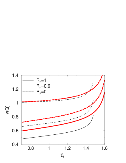
$$\left\langle(\Delta Q)^{2}\right\rangle = \left\langle(\Delta N_{+})^{2}\right\rangle+\left\langle(\Delta N_{-})^{2}\right\rangle$$ (20)

$$- 2R_{F}(T,\Delta y)\left\langle\Delta N_{+}\Delta N_{-}\right\rangle$$

The dependence of the observed fluctuations on $R_{F}$ is shown in Fig. 4, left panel.

We note two effects not considered here and believed to be unimportant:
1) the rescattering after formation is unlikely to alter $R_{F}$, since the typical momentum exchange in each collision the exchanged momentum $\left\langle q\right\rangle\sim T/3$ tends to be considerably softer than what is required to bring particles outside the acceptance region (in most decays, the characteristic momentum of the decay products in a resonance’s rest frame $p^{*}$ tends to be significantly larger than this value);
2) The higher-momentum pseudo-elastic “regeneration” processes, where detectable resonances would be created, are also unlikely to modify $R_{F}$ since, by local thermal equilibrium, two particles coming into the acceptance region through kinematically allowed pseudo-elastic interactions will be balanced out by two particles originally in the acceptance region which come out as a result of the re-interaction.
Thus, a measurement of fluctuations can still be relied upon to gauge the number of resonances present at chemical freeze-out. This underscores the importance of fluctuations as a probe for freeze-out dynamics.

We now obtain $R_{F}$ for a azimuthally symmetric perfect detector having a pseudo-rapidity coverage $\Delta\eta$. We shall follow the formalism in Ani85 to relate the resonance’s rest frame (denoted by $*$) to the lab frame.

For both particles $+$ and $-$ to be within the detector’s acceptance region, $-\Delta\eta/2<\eta_{+},\eta_{-}<\Delta\eta/2$ where

$$\eta_{\pm}=\frac{1}{2}\log\left(\frac{\sqrt{E_{\pm}^{2}-m_{\pm}^{2}}-p_{L\pm}}{\sqrt{E_{\pm}^{2}-m_{\pm}^{2}}+p_{L\pm}}\right)=\ln\left[\cot\left(\frac{\theta_{\pm}}{2}\right)\right]$$ (21)

If all angular dependence in the resonance’s decay matrix elements is neglected (a valid approximation if many resonances are produced, with an approximately azimuthally invariant distribution)the fraction of detectable $+-$ pairs will then be simply given by a phase space integral

$$\Omega_{+-}(\eta_{R},p_{TR})=\int\frac{d^{3}p^{*}_{+}}{E^{*}_{+}}\frac{d^{3}p^{*}_{-}}{E^{*}_{-}}\prod_{i}\frac{d^{3}p^{*}_{i}}{E^{*}_{i}}\Theta_{+-}$$ (22)

where:

$$\ \Theta_{+-}=\Theta\left[\eta_{+}-\frac{\Delta\eta}{2}\right]\Theta\left[\eta_{+}+\frac{\Delta\eta}{2}\right]\Theta\left[\eta_{-}-\frac{\Delta\eta}{2}\right]\Theta\left[\eta_{-}+\frac{\Delta\eta}{2}\right]$$

and the function $\Theta(z)$ is the usual step function

$$\ \begin{array}[]{cc}\Theta(z)=0&z<0\\ \Theta(z)=1&z>0\\ \end{array}$$

Now, for two body decays this reduces to

$$\Omega_{+-}(\eta_{R},p_{TR})=\frac{1}{4\pi}\int_{0}^{2\pi}d\phi\int_{0}^{1}d\left(\frac{p_{L}^{*}}{p^{*}}\right)\Theta_{+-}$$ (23)

while for three body decays we use the Monte-Carlo routine MAMBO mambo to generate points in phase space.

Figure 4: (Color online) Left: Sensitivity of the charge fluctuation measure on $R_{F}$, the fraction of resonance decay products which remains in the detector acceptance window (c.f. Eq.(20)). Thin black lines denote $T=170$ MeV, thick red lines $T=140$ MeV. Right: Acceptance fraction for different resonance decays as a function of the inverse slope $b$ (c.f. Eq.(27)) and the detector pseudo-rapidity acceptance $\Delta\eta$ (NB: $\eta$ in this context means the pseudo-rapidity. Not to be confused with the decay of the $\eta$ particle, shown on the right panel of the image). Acceptance regions of $\Delta\eta=6,4,2,1,0.5,0.1$ are considered, top to bottom in descending order

To calculate $\eta_{+}$ and $\eta_{-}$ from the resonance rest frame kinematic variables we Lorentz-transform to the lab frame, and get Ani85

$$p_{L\pm}=\pm p^{*}_{L\pm}+\frac{p_{LR}}{m_{R}}\left(E^{*}_{\pm}+\frac{\vec{p^{*}}.\vec{p_{R}}}{E_{R}+m_{R}}\right)$$ (24)

$$p_{T\pm}=\pm p^{*}_{T\pm}+\frac{p_{TR}}{m_{R}}\left(E^{*}_{\pm}+\frac{\vec{p^{*}}.\vec{p_{R}}}{E_{R}+m_{R}}\right)$$ (25)

To get an over-all fraction of accepted resonances which will enter Eq.(20) , one has to convolute Eq.(22) with a resonance distribution function in momentum space

$$R_{F}=\int_{0}^{\infty}dp_{TR}\int_{-\Delta\eta/2}^{\Delta\eta/2}d\eta_{R}P(\eta_{R},p_{TR})\Omega_{+-}(\eta_{R},p_{TR})$$ (26)

where $P(\eta_{R},p_{TR})$ is a suitable distribution function for resonances normalized to unity. A suitable function in the low energy region at mid-rapidity is

$$P(\eta_{R},p_{TR})=\frac{m_{TR}^{\alpha}e^{-bm_{TR}}}{\Delta\eta_{R}\int_{m}^{\infty}dm_{TR}m_{TR}^{\alpha}e^{-bm_{TR}}}$$ (27)

We have performed this integral using a Monte-Carlo method. The result is shown in the right panel of Fig. 4. We note that the most abundant resonance decays for charge fluctuations do not depend strongly on the inverse slope parameter $b^{-1}$: Going from $b^{-1}=200$ MeV to $b^{-1}=300$ MeV while staying in the same rapidity bin changes the $\rho\rightarrow\pi\pi$ correction by at most 5 $\%$, and the less abundant but more sensitive $\eta\rightarrow\pi^{+}\pi^{-}\pi^{0}$ correction by no more than 20$\%$.

Thus, $\Delta\eta$ should be as small as possible, statistics permitting, due to the not easily controllable corrections described in section V.1. A subsequent SHM analysis of the experimental data can than calculate $R_{F}$ for each resonance decay important for charge fluctuations. Hence, a $v(Q)$ , properly corrected for experimental acceptance, can be computed from SHM parameters via Eqs.(3) and (20), and fed into Fig. 1 and similar figures or fits ourfluct1 ; ourfluct2 ; ourfluct3 . The computational tools needed to perform such an analysis have been published separately as open-source software share2 .

It is important to underline that to perform this analysis it is not necessary to understand the full freeze-out dynamics of the fireball (local temperature, flow field, hadronization hypersurface). It is enough to have a sensible parametrization of $b^{-1}$ in terms of particle mass. This function is commonly obtained from particle spectra at thermal freeze-out slopemass , and is approximately linear in particle mass. The question is weather we can extrapolate $b^{-1}$ to chemical freeze-out conditions with enough precision in a model-independent way. The relatively mild dependence of $R_{F}$ on $b^{-1}$, together with the fact that hadronic re-interaction decreases the temperature and increases the flow and the high viscosity of the hadron gas hadvisc makes us confident that we can do it.

VI Summary and conclusions

We have studied in this work how a simultaneous measurement of charge fluctuations and a ratio such as $\Lambda/K^{-}$ can differentiate between chemical equilibrium and non-equilibrium freeze-out, and to constrain the magnitude of the deviation from equilibrium as well as the freeze-out temperature. Our results show that it is possible to distinguish the chemical equilibrium freeze-out condition $\gamma_{q}=1$ Rafelski:2004dp with $T=170$ MeV bdm ) from the chemical non-equilibrium freeze-out condition $\gamma_{q}=1.6$ Rafelski:2003ju ; Rafelski:2004dp . This is mainly due to the increase in the fluctuations inherent to an oversaturated Bose gas, see Eq.(12).

We have further discussed the dependence of two-particle correlations on the detector acceptance region, and have shown that it can be calculated to a reasonable precision in a model-independent way. The “right” experimental detector acceptance for a detailed study of fluctuations, therefore, is one that is appropriately small yet sizable to ensure the appropriate ensemble under study is Grand-Canonical, provided that acceptance corrections to resonance decays are properly taken into account using the methods described in section V.2. Quantitative corrections to Grand Canonical yield/fluctuation relations for the best fit parameters can be estimated quantitatively via Eq.(14)

Provided the detector acceptance region for a given fluctuation measurement is published, Eq.(26) can be used to calculate a correction coefficient $R_{F}$ to the $\left\langle N_{+}N_{-}\right\rangle$ correlation for each decay of a neutral resonance. Using a calculated $R_{F}$ for each resonance decay, together with the statistical model parameters, the charge fluctuation variable $v(Q)$ can be calculated from Eqs.(3) and (20). This $v(Q)$ will still retain the sensitivities to temperature and $\gamma_{q}$ demonstrated in section IV, since $\gamma_{q}$ impacts the primordial fluctuation terms rather than the correlation. It can therefore be used, together with a measurement such as $\Lambda/K^{-}$ as in Fig. 3, or within a fit as in ourfluct1 ; ourfluct2 ; ourfluct3 , to test the validity of the statistical model, unambiguously constrain its parameters, and differentiate between the high-temperature equilibrium and supercooled over-saturated freeze-out scenarios.

It is our intent to perform a complete data analysis as outlined here, including consideration of acceptance corrections and of resonance decays, once final RHIC fluctuation data becomes available.

VI.1 Acknowledgments

GT thanks C. Gale, L. Shi, V. Topor Pop, A. Bourque, Wojciech Broniowski, Wojciech Florkowski and Mark Gorenstein for stimulating discussions and the Tomlinson foundation for support. S.J. thanks RIKEN BNL Center and U.S. Department of Energy [DE-AC02-98CH10886] for providing facilities essential for the completion of this work. Work supported in part by grants from the U.S. Department of Energy (J.R. by DE-FG02-04ER41318), the Natural Sciences and Engineering research council of Canada, the Fonds Nature et Technologies of Quebec.

References

- (1) S. Jeon and V. Koch, “Event-by-event fluctuations,” arXiv:hep-ph/0304012, In: Hwa, R.C. (ed.) et al.: Quark gluon plasma, Singapoire 2004, pp 430-490.
- (2) S. Jeon, V. Koch, K. Redlich and X. N. Wang, Nucl. Phys. A 697, 546 (2002).
- (3) S. Jeon and V. Koch, Phys. Rev. Lett. 83, 5435 (1999).
- (4) S. Jeon and V. Koch, Phys. Rev. Lett. 85, 2076 (2000).
- (5) M. Asakawa, U. W. Heinz and B. Muller, Phys. Rev. Lett. 85, 2072 (2000).
- (6) S. Mrowczynski, Phys. Rev. C 57, 1518 (1998).
- (7) C. Pruneau, S. Gavin and S. Voloshin, Phys. Rev. C 66, 044904 (2002).
- (8) J. Zaranek, Phys. Rev. C 66, 024905 (2002)
- (9) Q. H. Zhang, V. Topor Pop, S. Jeon and C. Gale, Phys. Rev. C 66, 014909 (2002)
- (10) J. G. Reid [STAR Collaboration], Nucl. Phys. A 698 (2002) 611.
- (11) J. Adams et al. [STAR Collaboration], Phys. Rev. C 68, 044905 (2003).
- (12) K. Adcox et al. [PHENIX Collaboration], Phys. Rev. Lett. 89, 082301 (2002).
- (13) A. Bialas and R. C. Hwa, Phys. Lett. B 253, 436 (1991).
- (14) S. Hegyi and T. Csorgo, Phys. Lett. B 296, 256 (1992).
- (15) E. Fermi, Prog. Theor. Phys. 5, 570 (1950).
- (16) I. Pomeranchuk, Proc. USSR Academy of Sciences 43, 889 (1951).
- (17) L. D. Landau, Izv. Akad. Nauk Ser. Fiz. 17 (1953) 51.
- (18) R. Hagedorn, Suppl. Nuovo Cimento 2, 147 (1965).
- (19) V. V. Begun, M. I. Gorenstein, A. P. Kostyuk and O. S. Zozulya, arXiv:nucl-th/0410044.
- (20) V. V. Begun, M. Gazdzicki, M. I. Gorenstein and O. S. Zozulya, Phys. Rev. C 70, 034901 (2004).
- (21) J. Cleymans, K. Redlich, Phys. Rev. C 60, 054908 (1999).
- (22) See, for example, K. Huang, Statistical Mechanics, John Wiley and Sons, Second edition.
- (23) J. Letessier and J. Rafelski, Cambridge Monogr. Part. Phys. Nucl. Phys. Cosmol. 18, 1 (2002), see section 19.3.
- (24) J. Rafelski, J. Letessier, Acta Phys. Polon. B 34, 5791 (2003). J. Rafelski, J. Letessier, J. Phys. G 30, S1 (2004).
- (25) J. Rafelski and M. Danos, Phys. Lett. B 192, 432 (1987).
- (26) R. L. Thews, M. Schroedter and J. Rafelski, Phys. Rev. C 63, 054905 (2001) [arXiv:hep-ph/0007323].
- (27) F. Becattini, plasma in Phys. Rev. Lett. 95, 022301 (2005) [arXiv:hep-ph/0503239].
- (28) J. Rafelski and J. Letessier, Phys. Rev. Lett. 85, 4695 (2000).
- (29) J. Letessier and J. Rafelski, Int. J. Mod. Phys. E 9, 107, (2000).
- (30) J. Rafelski, J. Letessier, G. Torrieri, arXiv:nucl-th/0412072, Phys. Rev. C (2005) in press.
- (31) J. Letessier and J. Rafelski, arXiv:nucl-th/0504028.
- (32) F. Becattini, M. Gazdzicki, A. Keranen, J. Manninen and R. Stock, Phys. Rev. C 69, 024905 (2004).
-
(33)
G. Torrieri, W. Broniowski, W. Florkowski, J. Letessier, J. Rafelski, S. Steinke,
Comp. Phys. Com. 167, 229 (2005), see also:
www.physics.arizona.edu/torrieri/SHARE/share.html - (34) G. Torrieri, S. Jeon, J. Letessier and J. Rafelski, arXiv:nucl-th/0603026.
- (35) P. Braun-Munzinger, D. Magestro, K. Redlich and J. Stachel, Phys. Lett. B 518, 41 (2001).
- (36) G. Torrieri, S. Jeon and J. Rafelski, arXiv:nucl-th/0510024.
- (37) G. Torrieri, S. Jeon and J. Rafelski, arXiv:nucl-th/0509077.
- (38) G. Torrieri, S. Jeon and J. Rafelski, arXiv:nucl-th/0509067.
- (39) V.V. Anisovich, M.N. Kobrinsky, J. Nyiri and Y. Shabelski, Quark model and high energy collisions, (World Scientific, Singapore, 1985).
- (40) R. Kleiss and W. J. Stirling, Nucl. Phys. B 385, 413 (1992).
- (41) F. Antinori et al. [WA97 Collaboration], Eur. Phys. J. C 14, 633 (2000).
- (42) E. L. Bratkovskaya, S. Soff, H. Stoecker, M. van Leeuwen and W. Cassing, Phys. Rev. Lett. 92, 032302 (2004) [arXiv:nucl-th/0307098].