Phase structure of a two-fluid bosonic system

Abstract

The phase diagram of a two-fluid bosonic system is investigated. The proton-neutron interacting boson model (IBM-2) possesses a rich phase structure involving three control parameters and multiple order parameters. The surfaces of quantum phase transition between spherical, axially-symmetric deformed, and $\mathrm{SU}_{\pi\nu}^{*}(3)$ triaxial phases are determined, and the evolution of classical equilibrium properties across these transitions is investigated. Spectroscopic observables are considered in relation to the phase diagram.

and

1 Introduction

The phase structure of quantum many-body systems has in recent years been a subject of great experimental and theoretical interest. Models based upon algebraic Hamiltonians are well-suited to the study of phase transitions. They possess a well-defined classical limit [1], allowing classical order parameters to be determined. And for certain specific forms of their Hamiltonians, algebraic models exhibit dynamical symmetries, which correspond to qualitatively distinct ground-state equilibrium configurations. These constitute the phases of the system [2]. Algebraic models have found extensive application to the spectroscopy of many-body systems, including nuclei [3] and molecules [4].

In the present work, the phase structure of a system comprised of two interacting fluids is investigated. The phase structure of one-fluid algebraic models, especially the interacting boson model (IBM) [3] for nuclei, has been studied in detail [5, 2]. However, algebraic models may also be used to describe multi-fluid systems, with multiple interacting constituent species. While one-fluid systems are described by a single elementary Lie algebra, usually $\mathrm{U}(n)$, multi-fluid systems are described by a coupling of such Lie algebras, $\mathrm{U}_{1}(n)\otimes\mathrm{U}_{2}(n)\otimes\cdots$ [3, 4]. A richer phase structure arises for multi-fluid models, not just from the greater number of control and order parameters afforded by the more complicated model, but more fundamentally from the coupling of multiple subsystems, each of which can exist in a different phase or can drive phase transitions of the composite system.

Here we consider the proton-neutron interacting boson model (IBM-2) [6, 7, 8, 3], in which proton pairs and neutron pairs are treated as distinct constituents. The one-fluid IBM, with $\mathrm{U}(6)$ algebraic structure, has three dynamical symmetries, separated by first and second order phase transitions [5, 2]. The IBM-2, with $\mathrm{U}(6)\otimes\mathrm{U}(6)$ algebraic structure, supports four dynamical symmetries [9, 10]. Its phase diagram is therefore more involved and is found to possess qualitatively new features. Due to the complexity of the problem, a combination of analytic and numerical methods have been applied in the present work. Preliminary results were reported in Refs. [11, 12]. Numerical studies of the IBM-2 phase structure have also been carried out by Arias, Dukelsky, and García-Ramos [13, 14].

The IBM-2 and its classical limit are summarized in Sec. 2. The phase diagram of the IBM-2 is first investigated for an essential Hamiltonian with few parameters, for which the most complete analytic results are obtained (Sec. 3). The treatment is then extended to a more general Hamiltonian, incorporating realistic quadrupole and Majorana interactions (Sec. 4). Connection of the IBM-2 phase diagram with experimental data requires knowledge of the spectroscopic predictions across the phase transitions. These are addressed in Sec. 5.

The results of Sec. 5 are of relevance in the search for triaxial shapes in nuclei. Specific signatures of two-fluid triaxial deformation, and of the phase transition between axially symmetric and triaxial structure, are presented. Those signatures involving low-lying states are applicable both to current experiments and to experiments planned for next generation radioactive beam facilities. Those involving the high-lying magnetic dipole mode might be most directly investigated through resonance fluorescence experiments at high intensity gamma-ray facilities.

2 IBM-2 definition and classical limit

2.1 Hamiltonian

Let us first summarize the IBM-2 Hamiltonian and the dynamical symmetries it supports. Operators in the IBM-2 are constructed from the generators of the group $\mathrm{U}_{\pi}(6)\otimes\mathrm{U}_{\nu}(6)$, realized in terms of the boson creation operators $s_{\rho,0}^{{\dagger}}$ and $d_{\rho,\mu}^{{\dagger}}$ (where $\rho$ represents $\pi$ or $\nu$, and $\mu$$=$$-2,\ldots,2$) and their associated annihilation operators, acting on a basis of good boson numbers $N_{\pi}$ and $N_{\nu}$. The physically dominant interactions are contained in a Hamiltonian

$$H=\varepsilon_{\pi}\hat{n}_{d\pi}+\varepsilon_{\nu}\hat{n}_{d\nu}+\kappa_{\pi\pi}\hat{Q}_{\pi}^{\chi_{\pi}}\cdot\hat{Q}_{\pi}^{\chi_{\pi}}+\kappa_{\pi\nu}\hat{Q}_{\pi}^{\chi_{\pi}}\cdot\hat{Q}_{\nu}^{\chi_{\nu}}+\kappa_{\nu\nu}\hat{Q}_{\nu}^{\chi_{\nu}}\cdot\hat{Q}_{\nu}^{\chi_{\nu}}+\lambda\hat{M},$$ (2.1)

where $\hat{n}_{d\rho}\equiv d_{\rho}^{{\dagger}}\cdot\tilde{d}_{\rho}$, $\hat{Q}_{\rho}^{\chi_{\rho}}\equiv(s_{\rho}^{{\dagger}}\times\tilde{d}_{\rho}+d_{\rho}^{{\dagger}}\times\tilde{s}_{\rho})^{(2)}+\chi_{\rho}(d_{\rho}^{{\dagger}}\times\tilde{d}_{\rho})^{(2)}$, $\hat{M}\equiv-2\sum_{k=1,3}(d_{\pi}^{\dagger}\times d_{\nu}^{\dagger})^{(k)}\cdot(\tilde{d}_{\pi}\times\tilde{d}_{\nu})^{(k)}+(s_{\pi}^{\dagger}\times d_{\nu}^{\dagger}-s_{\nu}^{\dagger}\times d_{\pi}^{\dagger})^{(2)}\cdot(\tilde{s}_{\pi}\times\tilde{d}_{\nu}-\tilde{s}_{\nu}\times\tilde{d}_{\pi})^{(2)}$, and conventional spherical tensor coupling notation (e.g., Ref. [15]) has been used. This Hamiltonian contains one-fluid contributions, arising from like-nucleon pairing ($\hat{n}_{d\rho}$) and quadrupole ($\hat{Q}_{\rho}\cdot\hat{Q}_{\rho}$) interactions, as well as two-fluid coupling terms, arising from proton-neutron quadrupole ($\hat{Q}_{\pi}\cdot\hat{Q}_{\nu}$) and Majorana ($\hat{M}$) interactions. The physically relevant ranges of the Hamiltonian parameters are $\varepsilon_{\rho}\geq 0$, $\kappa_{\rho\rho^{\prime}}\leq 0$, $-\sqrt{7}/2\leq\chi_{\rho}\leq\sqrt{7}/2$, and $\lambda\geq 0$ [3].

A dynamical symmetry occurs when, for certain values of the parameters, the Hamiltonian is constructed from the Casimir operators of a chain of subalgebras of $\mathrm{U}_{\pi}(6)\otimes\mathrm{U}_{\nu}(6)$. Three of the IBM-2 dynamical symmetries occur for $\chi_{\pi}=\chi_{\nu}$ and have direct analogues in the one-fluid IBM [9]. When $\kappa_{\pi\pi}=\kappa_{\pi\nu}=\kappa_{\nu\nu}=0$, the $\mathrm{U}_{\pi\nu}(5)$ dynamical symmetry is realized, with subalgebra chain

$$\mathrm{U}_{\pi}(6)\otimes\mathrm{U}_{\nu}(6)\supset\mathrm{U}_{\pi}(5)\otimes\mathrm{U}_{\nu}(5)\supset\mathrm{U}_{\pi\nu}(5)\supset\mathrm{SO}_{\pi\nu}(3).$$ (2.2)

The geometric interpretation is that the proton and neutron fluids undergo oscillations about a spherical equilibrium configuration. Parameter values $\varepsilon_{\pi}=\varepsilon_{\nu}=0$ with $\chi_{\pi}=\chi_{\nu}=0$ produce the $\mathrm{SO}_{\pi\nu}(6)$ dynamical symmetry

$$\mathrm{U}_{\pi}(6)\otimes\mathrm{U}_{\nu}(6)\supset\mathrm{SO}_{\pi}(6)\otimes\mathrm{SO}_{\nu}(6)\supset\mathrm{SO}_{\pi\nu}(6)\supset\mathrm{SO}_{\pi\nu}(3),$$ (2.3)

yielding deformed, $\gamma$-unstable structure. And $\varepsilon_{\pi}=\varepsilon_{\nu}=0$ with $\chi_{\pi}=\chi_{\nu}=-\sqrt{7}/2$ gives the $\mathrm{SU}_{\pi\nu}(3)$ dynamical symmetry

$$\mathrm{U}_{\pi}(6)\otimes\mathrm{U}_{\nu}(6)\supset\mathrm{SU}_{\pi}(3)\otimes\mathrm{SU}_{\nu}(3)\supset\mathrm{SU}_{\pi\nu}(3)\supset\mathrm{SO}_{\pi\nu}(3),$$ (2.4)

for which prolate axially symmetric structure is obtained. The complementary case $\chi_{\pi}=\chi_{\nu}=+\sqrt{7}/2$, giving oblate axially symmetric structure, is distinguished by the notation $\overline{\mathrm{SU}_{\pi\nu}(3)}$.

However, a symmetry special to the IBM-2, denoted $\mathrm{SU}_{\pi\nu}^{*}(3)$, is obtained for $\varepsilon_{\pi}=\varepsilon_{\nu}=0$ with $\chi_{\pi}=-\sqrt{7}/2$ and $\chi_{\nu}=+\sqrt{7}/2$ [10, 16, 17, 18, 19]. In this case the Hamiltonian is constructed from Casimir operators of the subalgebra chain

$$\mathrm{U}_{\pi}(6)\otimes\mathrm{U}_{\nu}(6)\supset\mathrm{SU}_{\pi}(3)\otimes\overline{\mathrm{SU}_{\nu}(3)}\supset\mathrm{SU}_{\pi\nu}^{*}(3)\supset\mathrm{SO}_{\pi\nu}(3).$$ (2.5)

The equilibrium configuration consists of a proton fluid with axially symmetric prolate deformation coupled to a neutron fluid with axially symmetric oblate deformation, with their symmetry axes orthogonal to each other [10, 20, 21]. This yields an overall composite nuclear shape with triaxial deformation, as shown in Fig. 1. To avoid ambiguity, we shall adopt here the notation $\overline{\mathrm{SU}_{\pi\nu}^{*}(3)}$ for the complementary case $\chi_{\pi}=+\sqrt{7}/2$ and $\chi_{\nu}=-\sqrt{7}/2$, in which the proton and neutron deformations are interchanged.

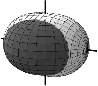
Figure 1: Geometrical interpretation of the equilibrium structure for the $\mathrm{SU}_{\pi\nu}^{*}(3)$ dynamical symmetry. A prolate deformed proton fluid (light gray) and oblate deformed neutron fluid (dark gray) are coupled with orthogonal symmetry axes. Figure adapted from Ref. [22].

2.2 Coherent state energy surface

The phase structure of an algebraic model is determined from the classical limit of the model, which is obtained through the coherent state formalism [23, 1, 24]. A coherent state of good boson number is constructed, and the parameters of this state are directly related to the classical coordinates of the system. This coherent state is used as a variational trial state: the global minimum of the energy surface $\mathcal{E}\equiv\langle H\rangle$ is used to determine the ground state energy and equilibrium classical coordinates of the system. In the limit of infinite boson number, the coherent state variational energy converges to the true ground state energy [23, 1]. Detailed coherent state analyses of the one-fluid IBM may be found in Refs. [25, 26, 5, 27, 2, 28, 29, 30].

Once the equilibrium properties of the model have been established, ground state phase transitions can be identified and categorized according to the Ehrenfest classification [31]: a phase transition is first order if the first derivative of the system’s energy is discontinuous with respect to the control parameter being varied, second order if the second derivative is discontinuous, etc. Where the system’s energy is obtained, as in the present classical analysis, as the global minimum of an energy function $\mathcal{E}$, a first order transition is usually associated with a discontinuous jump in the equilibrium coordinates (“order parameters”) between distinct competing minima. Second or higher order transitions are associated instead with a continuous evolution of the equilibrium coordinates, as when an initially solitary global minimum becomes unstable (possessing a vanishing second derivative with respect to some coordinate) and evolves into two or more minima. It should be noted that, whenever the order of a phase transition is obtained by numerical analysis, application of the Ehrenfest criterion is limited by the ability to numerically resolve sufficiently small discontinuities. This is especially a consideration for points of first-order transition very close to a point of second-order transition. Moreover, problems with the classification scheme, not addressed here, may arise at the boundaries of the parameter space or when the Hamiltonian possesses additional symmetries.

For a two-fluid model, the boson number for each constituent fluid is conserved separately. The coherent state is constructed not only with good total boson number but with good boson number for each fluid. For the IBM-2, the number operators are $\hat{N_{\rho}}\equiv s_{\rho,0}^{\dagger}s_{\rho,0}+\sum_{\mu=-2}^{2}d_{\rho,\mu}^{\dagger}d_{\rho,\mu}$. The IBM-2 coherent state [26, 32, 33, 34] is defined in terms of proton and neutron condensate bosons

$$B_{\rho c}^{\dagger}\equiv\frac{1}{(1+|\alpha_{\rho}^{(2)}|^{2})^{1/2}}\Bigl{(}s_{\rho,0}^{\dagger}+\sum_{\mu=-2}^{2}\alpha_{\rho,\mu}^{(2)}d_{\rho,\mu}^{\dagger}\Bigr{)},$$ (2.6)

where $|\alpha_{\rho}^{(2)}|\equiv(\sum_{\mu=-2}^{2}\alpha_{\rho,\mu}^{(2)\,*}\alpha_{\rho,\mu}^{(2)})^{1/2}$, as

$$|N_{\pi},\alpha^{(2)}_{\pi};N_{\nu},\alpha^{(2)}_{\nu}\rangle\equiv\frac{1}{(N_{\pi}!)^{1/2}(N_{\nu}!)^{1/2}}\left(B_{\pi c}^{\dagger}\right)^{N_{\pi}}\left(B_{\nu c}^{\dagger}\right)^{N_{\nu}}\,|0\rangle.$$ (2.7)

The $\alpha^{(2)}_{\rho,\mu}$ are interpreted geometrically as quadrupole shape variables [35] for the proton and neutron fluids. They are related to the four deformation parameters ($\beta_{\pi}$, $\gamma_{\pi}$, $\beta_{\nu}$, and $\gamma_{\nu}$) and to the six Euler angles ($\theta_{1\pi}$, $\theta_{2\pi}$, $\theta_{3\pi}$, $\theta_{1\nu}$, $\theta_{2\nu}$, and $\theta_{3\nu}$) specifying the orientations of the proton and neutron intrinsic frames by

$$\alpha_{\rho,\mu}^{(2)}=\beta_{\rho}\cos\gamma_{\rho}D^{2\,*}_{\mu 0}(\theta_{1\rho},\theta_{2\rho},\theta_{3\rho})\\ +\frac{1}{\sqrt{2}}\beta_{\rho}\sin\gamma_{\rho}\bigl{[}D^{2\,*}_{\mu 2}(\theta_{1\rho},\theta_{2\rho},\theta_{3\rho})+D^{2\,*}_{\mu-2}(\theta_{1\rho},\theta_{2\rho},\theta_{3\rho})\bigr{]},$$ (2.8)

where $D_{M^{\prime}M}^{J}$ is the Wigner $D$ function [36].

Calculation of the expectation value of $H$ with respect to the coherent state (2.7) yields an energy surface $\mathcal{E}\equiv\langle N_{\pi},\alpha^{(2)}_{\pi};N_{\nu},\alpha^{(2)}_{\nu}|H|N_{\pi},\alpha^{(2)}_{\pi};N_{\nu},\alpha^{(2)}_{\nu}\rangle$. By rotational invariance, $\mathcal{E}$ can only depend upon the relative Euler angles $\vartheta_{i}$ between the proton and neutron fluid intrinsic frames, not the $\theta_{i\pi}$ and $\theta_{i\nu}$ separately. For evaluation of $\mathcal{E}$, the Euler angles may thus simply be chosen to be $\theta_{i\pi}=0$ and $\theta_{i\nu}=\vartheta_{i}$. Investigations of the IBM-2 coherent state energy surface have been carried out in Refs. [37, 20, 21].

The expectation value with respect to the IBM-2 coherent state of an operator constructed from the boson operators of one fluid only (e.g., $\hat{n}_{d\pi}$ or $\hat{Q}_{\pi}\cdot\hat{Q}_{\pi}$) can be calculated as in the one-fluid IBM, by the methods of Refs. [26, 28]. The expectation values of the one-fluid operators appearing in (2.1) are [28]

$$\langle\hat{n}_{d\rho}\rangle =\frac{N_{\rho}\beta_{\rho}^{2}}{1+\beta_{\rho}^{2}}$$ (2.9)

$$\langle\hat{Q}^{\chi_{\rho}}_{\rho}\cdot\hat{Q}^{\chi_{\rho}}_{\rho}\rangle =\frac{N_{\rho}}{1+\beta_{\rho}^{2}}\Bigl{[}5+(1+\chi_{\rho}^{2})\beta_{\rho}^{2}\Bigr{]}$$ (2.10)

$$\qquad\qquad\qquad+\frac{N_{\rho}(N_{\rho}-1)}{(1+\beta_{\rho}^{2})^{2}}\Bigl{[}4\beta_{\rho}^{2}-4\sqrt{\frac{2}{7}}\chi_{\rho}\beta_{\rho}^{3}\cos 3\gamma_{\rho}+\frac{2}{7}\chi_{\rho}^{2}\beta_{\rho}^{4}\Bigr{]}.$$

The expectation value of a two-fluid operator constructed as the scalar product of one-fluid operators (e.g., $\hat{Q}_{\pi}\cdot\hat{Q}_{\nu}$) can be obtained using a factorization result [21, (C1)]. However, for more complicated operators, the general method presented in Appendix A provides a convenient means of calculation. The expectation value of $\hat{Q}_{\pi}\cdot\hat{Q}_{\nu}$ is a function of all seven possible coordinates ($\beta_{\pi}$, $\gamma_{\pi}$, $\beta_{\nu}$, $\gamma_{\nu}$, $\vartheta_{1}$, $\vartheta_{2}$, and $\vartheta_{3}$),

$$\langle\hat{Q}_{\pi}^{\chi_{\pi}}\cdot\hat{Q}_{\nu}^{\chi_{\nu}}\rangle=\frac{N_{\pi}N_{\nu}}{(1+\beta_{\pi}^{2})(1+\beta_{\nu}^{2})}[\alpha_{\pi}^{(2)\,*}+\tilde{\alpha}_{\pi}^{(2)}+\chi_{\pi}(\alpha_{\pi}^{(2)\,*}\times\tilde{\alpha}_{\pi}^{(2)})^{(2)}]\\ \cdot[\alpha_{\nu}^{(2)\,*}+\tilde{\alpha}_{\nu}^{(2)}+\chi_{\nu}(\alpha_{\nu}^{(2)\,*}\times\tilde{\alpha}_{\nu}^{(2)})^{(2)}],$$ (2.11)

with the $\alpha_{\rho}^{(2)}$ as defined in Eqn. (2.8), which for vanishing Euler angles simplifies to

$$\langle\hat{Q}_{\pi}^{\chi_{\pi}}\cdot\hat{Q}_{\nu}^{\chi_{\nu}}\rangle=\frac{2N_{\pi}N_{\nu}\beta_{\pi}\beta_{\nu}}{7(1+\beta_{\pi}^{2})(1+\beta_{\nu}^{2})}\Bigl{[}14\cos(\gamma_{\pi}-\gamma_{\nu})+\chi_{\pi}\chi_{\nu}\beta_{\pi}\beta_{\nu}\cos(2\gamma_{\pi}-2\gamma_{\nu})\\ \qquad\qquad+\sqrt{14}[\chi_{\pi}\beta_{\pi}\cos(2\gamma_{\pi}+\gamma_{\nu})+\chi_{\nu}\beta_{\nu}\cos(\gamma_{\pi}+2\gamma_{\nu})]\Bigr{]}.$$ (2.12)

The expectation value of the Majorana operator is a complicated function of the coordinates. For vanishing Euler angles, it reduces to

$$\langle\hat{M}\rangle=\frac{N_{\pi}N_{\nu}}{(1+\beta_{\pi}^{2})(1+\beta_{\nu}^{2})}\bigl{[}\beta_{\pi}^{2}+\beta_{\nu}^{2}-2\beta_{\pi}\beta_{\nu}\cos(\gamma_{\pi}-\gamma_{\nu})+\beta_{\pi}^{2}\beta_{\nu}^{2}\sin^{2}(\gamma_{\pi}-\gamma_{\nu})\bigr{]}.$$ (2.13)

A detailed study of the possible equilibrium Euler angle and $\gamma_{\rho}$ values for the most general two-body IBM-2 Hamiltonian has been presented in Ref. [21]. So long as the multipole decomposition of the proton-neutron interaction contains no hexadecapole component [$(d_{\pi}^{\dagger}\times\tilde{d}_{\pi})^{(4)}\cdot(d_{\nu}^{\dagger}\times\tilde{d}_{\nu})^{(4)}$], it is found that the equilibrium configuration must have Euler angles which are vanishing or multiples of $\pi/2$. Thus, the proton and neutron intrinsic frames are “aligned”, to within a possible relabeling of axes. [For clarity, we note that in the $\mathrm{SU}_{\pi\nu}^{*}(3)$ equilibrium configuration (Fig. 1), even though the proton and neutron symmetry axes are orthogonal, the intrinsic frame coordinate axes are actually parallel, i.e., the Euler angles vanish. The proton ($\gamma_{\pi}=0$) symmetry axis is the $z$ axis, while the neutron ($\gamma_{\nu}=\pi/3$) symmetry axis is the $y$ axis.] If, instead, a hexadecapole contribution is present, “oblique” equilibrium configurations are possible. The operator $\hat{Q}_{\pi}\cdot\hat{Q}_{\nu}$ contains no hexadecapole component, but the Majorana operator does (Sec. 4.3). The IBM-2 is thus characterized by either four order parameters ($\beta_{\pi}$, $\gamma_{\pi}$, $\beta_{\nu}$, and $\gamma_{\nu}$) or seven order parameters ($\beta_{\pi}$, $\gamma_{\pi}$, $\beta_{\nu}$, $\gamma_{\nu}$, $\vartheta_{1}$, $\vartheta_{2}$, and $\vartheta_{3}$), depending upon the form of the proton-neutron interaction.

3 Phase structure for an essential Hamiltonian

3.1 The $F$-spin invariant Hamiltonian

A simple, schematic Hamiltonian which retains the essential dynamical symmetry features of the IBM-2, obtained as a special case of Eqn. (2.1), is

$$H=\varepsilon(\hat{n}_{d\pi}+\hat{n}_{d\nu})+\kappa(\hat{Q}_{\pi}^{\chi_{\pi}}+\hat{Q}_{\nu}^{\chi_{\nu}})\cdot(\hat{Q}_{\pi}^{\chi_{\pi}}+\hat{Q}_{\nu}^{\chi_{\nu}}).$$ (3.1)

This Hamiltonian is often preferred for theoretical studies due to its invariance under $F$-spin rotations (e.g., Ref. [38]) for ${\chi_{\pi}}={\chi_{\nu}}$. To make the analysis of the IBM-2 phase structure as transparent as possible, let us first consider in detail this $F$-spin invariant Hamiltonian before proceeding in Section 4 to the more general form. It is also convenient for the moment to restrict attention to the case $N_{\pi}=N_{\nu}$.

To obtain the classical limit, it is necessary to take $N\rightarrow\infty$, where $N=N_{\pi}+N_{\nu}$. In this limit, the lower-order terms with respect to $N$ in Eqn. (2.10) become negligible, and it is seen that the quantities $\langle\hat{n}_{d\rho}\rangle$ are linear in $N$, while the $\langle\hat{Q}_{\rho}\cdot\hat{Q}_{\rho^{\prime}}\rangle$ are all quadratic in $N$. To prevent the $\langle\hat{n}_{d\rho}\rangle$ contributions from vanishing identically when the limit is taken, it is necessary to rescale the Hamiltonian coefficients by appropriate powers of $N$. It is thus convenient to reparametrize the Hamiltonian (3.1) as

$$H=\frac{1-\xi^{\prime}}{N}(\hat{n}_{d\pi}+\hat{n}_{d\nu})-\frac{\xi^{\prime}}{N^{2}}(\hat{Q}_{\pi}^{\chi_{\pi}}+\hat{Q}_{\nu}^{\chi_{\nu}})\cdot(\hat{Q}_{\pi}^{\chi_{\pi}}+\hat{Q}_{\nu}^{\chi_{\nu}}),$$ (3.2)

so that the energy function $\mathcal{E}$ is independent of $N$. This definition also condenses the full range of possible ratios $\varepsilon/\kappa$ onto the finite interval $0\leq\xi^{\prime}\leq 1$. An overall normalization parameter for $H$ has been discarded as irrelevant to the extremum structure of the energy surface.

There are three control parameters — $\xi^{\prime}$, $\chi_{\pi}$, and $\chi_{\nu}$ — for the Hamiltonian (3.2). It is convenient to alternatively introduce “scalar” and “vector” parameters $\chi_{S}$$\equiv$$\frac{1}{2}(\chi_{\pi}+\chi_{\nu})$ and $\chi_{V}$$\equiv$$\frac{1}{2}(\chi_{\pi}-\chi_{\nu})$. The parameter space is outlined in Fig. 2.

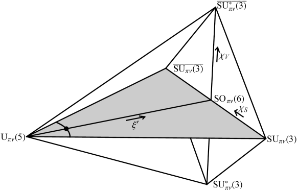
Figure 2: Parameter space for the $F$-spin invariant Hamiltonian of Eqn. (3.2). For $\chi_{V}=0$ (shaded plane) the analysis reduces to that for the one-fluid IBM (see text), yielding a point of second-order phase transition embedded in a curve (3.3) of first-order phase transition points. The axes cover ranges $0\leq\xi^{\prime}\leq 1$, $-\sqrt{7}/2\leq\chi_{S}\leq\sqrt{7}/2$, and $-\sqrt{7}/2\leq\chi_{V}\leq\sqrt{7}/2$. The $\chi_{S}$ and $\chi_{V}$ axes are scaled by $\xi^{\prime}$, so as to converge to a point at the $\mathrm{U}_{\pi\nu}(5)$ limit, where the Hamiltonian is independent of $\chi_{S}$ and $\chi_{V}$. Figure from Ref. [22].

For $\chi_{V}=0$, indicated by the shaded triangle in Fig. 2, the analysis essentially reduces to that for the one-fluid IBM. The equilibrium configuration occurs for $\beta_{\pi}=\beta_{\nu}(\equiv\beta)$ and $\gamma_{\pi}=\gamma_{\nu}=0$ and is identical to that obtained for the IBM Hamiltonian $H_{\text{IBM}}=[(1-\xi^{\prime})/N]\hat{n}_{d}-(\xi^{\prime}/N^{2})\hat{Q}^{\chi}\cdot\hat{Q}^{\chi}$, the phase structure of which is well known [5, 2], with $\chi=\chi_{S}$. For $\xi^{\prime}\leq 1/5$, the energy surface has a minimum at $\beta=0$. At $\xi^{\prime}=1/5$, this minimum becomes unstable with respect to $\beta$, i.e., $\partial^{2}\mathcal{E}/\partial\beta^{2}=0$. If $\chi=0$, this instability leads to a second-order transition between undeformed ($\beta=0$) and deformed ($\beta\neq 0$) structure at $\xi^{\prime}=1/5$. However, for any other value of $\chi$, the minimum at $\beta=0$ is preempted as global minimum by a distinct minimum with nonzero $\beta$ before $\xi^{\prime}=1/5$. This leads to a first-order phase transition, at a parameter value $\xi^{\prime}=\xi^{\prime}_{c}(\chi)$ given by

$$\xi^{\prime}_{c}(\chi)=\frac{1}{5+\frac{2}{7}\chi^{2}},$$ (3.3)

easily derived from Ref. [29, (2.9b)]. Thus, the point of second-order phase transition at $\xi^{\prime}=1/5$ and $\chi=0$ lies on a trajectory (3.3) of first-order transition points (Fig. 2).

It simplifies the analysis of the phase diagram for the remainder of the parameter space to note the presence of reflection symmetries with respect to the $\chi_{\rho}$ parameters. Each term contributing to $\mathcal{E}$ is seen by inspection of Eqns. (2.9), (2.10), and (2.12) to be invariant under a simultaneous transformation of coordinates and Hamiltonian parameters

$$\chi_{\pi}\rightarrow-\chi_{\pi},\qquad\chi_{\nu}\rightarrow-\chi_{\nu},\qquad\gamma_{\pi}\rightarrow\frac{\pi}{3}-\gamma_{\pi},\qquad\gamma_{\nu}\rightarrow\frac{\pi}{3}-\gamma_{\nu}.$$ (3.4)

Thus, the equilibrium deformation at a point $(\chi_{\pi},\chi_{\nu})$ in parameter space is simply related to that at the point $(-\chi_{\pi},-\chi_{\nu})$ by Eqn. (3.4). The phase diagram is symmetric under simultaneous negation of $\chi_{\pi}$ and $\chi_{\nu}$ or, equivalently, simultaneous negation of $\chi_{S}$ and $\chi_{V}$. Moreover, for the $F$-spin invariant Hamiltonian (3.2) with $N_{\pi}=N_{\nu}$, the numerical coefficients on corresponding proton and neutron terms in $\mathcal{E}$ are equal. Thus, $\mathcal{E}$ is symmetric under interchange of all proton and neutron variables, and the phase diagram is symmetric under interchange of $\chi_{\pi}$ and $\chi_{\nu}$ or, equivalently, negation of $\chi_{V}$.

3.2 The $\mathrm{SU}_{\pi\nu}(3)-\mathrm{SO}_{\pi\nu}(6)-\mathrm{SU}_{\pi\nu}^{*}(3)$ plane

Let us begin the investigation of the phase structure of the Hamiltonian (3.2) with an analytic study for $\xi^{\prime}=1$, corresponding to the rightmost plane of the parameter space diagram in Fig. 2. This plane encompasses the $\mathrm{SO}_{\pi\nu}(6)$, $\mathrm{SU}_{\pi\nu}(3)$, and $\mathrm{SU}_{\pi\nu}^{*}(3)$ dynamical symmetries.

Surrounding the $\mathrm{SU}_{\pi\nu}(3)$ dynamical symmetry is a region of parameter space in which the equilibrium deformations are axially symmetric ($\gamma_{\pi}=\gamma_{\nu}=0$), and a similar region surrounds the $\overline{\mathrm{SU}_{\pi\nu}(3)}$ dynamical symmetry ($\gamma_{\pi}=\gamma_{\nu}=\pi/3$). In either of these cases ($\gamma_{\pi}=\gamma_{\nu}=0$ or $\pi/3$), the energy surface can be written in an especially simple form in terms of the function $F$ defined in Eqn. (B.1),

$$\mathcal{E}(\beta_{\pi},\beta_{\nu})=-4\left[F\left(-\frac{1}{\sqrt{14}}\chi_{\pi};\sigma\beta_{\pi}\right)+F\left(-\frac{1}{\sqrt{14}}\chi_{\nu};\sigma\beta_{\nu}\right)\right]^{2},$$ (3.5)

where $\sigma\equiv\cos 3\gamma_{\rho}=\pm 1$. The energy function in (3.5) is minimized when the magnitude of the quantity within brackets is maximized. In the vicinity of $\mathrm{SU}_{\pi\nu}(3)$, including in the entire quadrant for which $\chi_{\pi}$ and $\chi_{\nu}$ are both negative, it follows from the results of Appendix B that the minimum in $\mathcal{E}(\beta_{\pi},\beta_{\nu})$ occurs at coordinate values

$$\beta_{\rho}=-\frac{\chi_{\rho}}{\sqrt{14}}+\Biggl{[}\Biggl{(}\frac{\chi_{\rho}}{\sqrt{14}}\Biggr{)}^{2}+1\Biggr{]}^{1/2}$$ (3.6)

with $\sigma=+1$ (i.e., $\gamma_{\pi}=\gamma_{\nu}=0$). Similary, in the vicinity of $\overline{\mathrm{SU}_{\pi\nu}(3)}$, including in the entire quadrant for which $\chi_{\pi}$ and $\chi_{\nu}$ are both positive, the minimum in $\mathcal{E}(\beta_{\pi},\beta_{\nu})$ occurs at coordinate values

$$\beta_{\rho}=-\frac{\chi_{\rho}}{\sqrt{14}}-\Biggl{[}\Biggl{(}\frac{\chi_{\rho}}{\sqrt{14}}\Biggr{)}^{2}+1\Biggr{]}^{1/2}$$ (3.7)

with $\sigma=-1$ (i.e., $\gamma_{\pi}=\gamma_{\nu}=\pi/3$). In either case, the value of the energy function at the global minimum is

$$\mathcal{E}=-\frac{1}{4}(\beta_{\pi}+\beta_{\nu})^{2},$$ (3.8)

with $\beta_{\pi}$ and $\beta_{\nu}$ given by Eqn. (3.6) or (3.7) as appropriate.

As $\chi_{\pi}$ and $\chi_{\nu}$ are varied away from their $\mathrm{SU}_{\pi\nu}(3)$ values, eventually axial equilibrium deformation gives way to triaxial deformation, with $\gamma_{\pi}$ and/or $\gamma_{\nu}$ nonzero. This transition occurs on the locus of points at which the minimum given by (3.6) first becomes unstable with respect to $\gamma$ deformation. Since $\mathcal{E}$ depends upon both $\gamma_{\pi}$ and $\gamma_{\nu}$, instablility occurs when the directional second derivative of $\mathcal{E}$ first vanishes along some “direction” in $(\gamma_{\pi},\gamma_{\nu})$ coordinate space, which may generally happen before either $\partial^{2}\mathcal{E}/\partial\gamma_{\pi}^{2}$ or $\partial^{2}\mathcal{E}/\partial\gamma_{\nu}^{2}$ vanishes individually. The equation describing the boundary curve in $\chi_{\pi}$ and $\chi_{\nu}$ is most compactly expressed in terms of the corresponding equilibrium values $\beta_{\pi}$ and $\beta_{\nu}$ from Eqn. (3.6) or  (3.7), as

$$1-\beta_{\pi}^{2}-\beta_{\nu}^{2}-2\beta_{\pi}\beta_{\nu}^{3}+3\beta_{\pi}^{2}\beta_{\nu}^{2}-2\beta_{\pi}^{3}\beta_{\nu}+2\beta_{\pi}^{3}\beta_{\nu}^{3}=0.$$ (3.9)

This curve is shown in Fig. 3. The direction in $(\gamma_{\pi},\gamma_{\nu})$ space in which the instability occurs, at any given point on this boundary, is given by

$$\frac{\gamma_{\pi}}{\gamma_{\nu}}=-\frac{1+\beta_{\pi}^{2}}{1+\beta_{\nu}^{2}}\frac{B}{2A}=-\frac{1+\beta_{\pi}^{2}}{1+\beta_{\nu}^{2}}\frac{2C}{B},$$ (3.10)

where

$$A \equiv 9\beta_{\pi}^{2}(\beta_{\pi}^{2}-1)+\beta_{\pi}\beta_{\nu}(2\beta_{\pi}^{2}-1)(\beta_{\pi}^{2}+1)$$ (3.11)

$$B \equiv-4\beta_{\pi}\beta_{\nu}(\beta_{\pi}^{2}-2)(\beta_{\nu}^{2}-2)$$

$$C \equiv 9\beta_{\nu}^{2}(\beta_{\nu}^{2}-1)+\beta_{\pi}\beta_{\nu}(2\beta_{\nu}^{2}-1)(\beta_{\nu}^{2}+1).$$

Along the $\mathrm{SU}_{\pi\nu}(3)$-$\mathrm{SU}_{\pi\nu}^{*}(3)$ line in particular, for which $\chi_{\pi}=-\sqrt{7}/2$, the transition occurs at $\chi_{\nu}\approx 0.4035$, obtained from Eqn. (3.9) as the root of a quartic equation. In this special case, the global minimum becomes soft purely with respect to $\gamma_{\nu}$ at fixed $\gamma_{\pi}=0$.

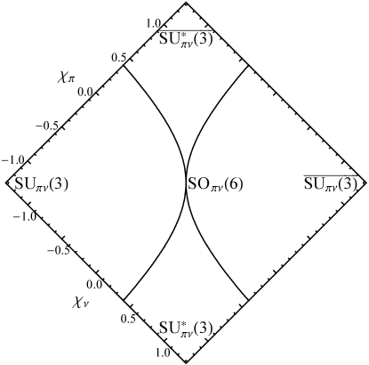
Figure 3: Phase diagram for the $\mathrm{SU}_{\pi\nu}(3)$-$\mathrm{SO}_{\pi\nu}(6)$-$\mathrm{SU}_{\pi\nu}^{*}(3)$ plane ($\xi^{\prime}=1$) in the parameter space of the Hamiltonian of (3.2), for $N_{\pi}=N_{\nu}$, showing the curve (3.9) of second-order phase transition. The diagram is rotated to allow more direct comparison with Figs. 2 and 4. Figure adapted from Ref. [12].

The analytic results of this section indicate a continuous transition between axially symmetric and triaxial structure on the curve (3.9). In Sec. 3.4 it is verified numerically that this transition is second, rather than higher, order, and that no prior phase transition to a distinct minimum occurs before the curve (3.9) is reached.

3.3 The transition between spherical and deformed equilibrium

The transition between spherical and deformed equilibrium for the IBM-2 for arbitrary $\chi_{V}$ is closely related to the transition which occurs in the special plane $\chi_{V}=0$ (shaded in Fig. 2). The energy function $\mathcal{E}(\xi^{\prime},\chi_{S},\chi_{V};\beta_{\pi},\gamma_{\pi},\beta_{\nu},\gamma_{\nu})$ obeys the identity

$$\mathcal{E}(\xi^{\prime},\chi_{S},\chi_{V};\beta,0,\beta,0)=\mathcal{E}(\xi^{\prime},\chi_{S},0;\beta,0,\beta,0),$$ (3.12)

i.e., for a deformation which is axial and has $\beta_{\pi}=\beta_{\nu}$, the value of $\mathcal{E}$ is independent of $\chi_{V}$. Recall that the equilibrium deformation for $\chi_{V}=0$ is always axial with $\beta_{\pi}=\beta_{\nu}$ (Sec. 3.1). It is straight-forward to demonstrate from these observations (see below) that a nonzero equilibrium deformation for the parameter point $(\xi^{\prime},\chi_{S})$ in the $\chi_{V}=0$ plane implies a nonzero equilibrium deformation for all the out-of-plane points $(\xi^{\prime},\chi_{S},\chi_{V})$. Thus, the $\xi^{\prime}$ value $\xi^{\prime}_{c}(\chi_{S},\chi_{V})$ for which the spherical-deformed transition occurs at a given $\chi_{S}$ and $\chi_{V}$ obeys, by Eqn. (3.3),

$$\xi^{\prime}_{c}(\chi_{S},\chi_{V})\leq\frac{1}{5+\frac{2}{7}\chi_{S}^{2}}.$$ (3.13)

The detailed argument proceeds as follows. Let the equilibium energy at a general point in parameter space be denoted by $\mathcal{E}_{0}(\xi^{\prime},\chi_{S},\chi_{V})$, and let $\beta_{0}(\xi^{\prime},\chi_{S})$ be the equilibrium value of $\beta_{\pi}$ and $\beta_{\nu}$ for $\chi_{V}=0$ as determined, e.g., from Ref. [29, (2.12)]. Then $\mathcal{E}_{0}(\xi^{\prime},\chi_{S},0)=\mathcal{E}[\xi^{\prime},\chi_{S},0;\beta_{0}(\xi^{\prime},\chi_{S}),0,\beta_{0}(\xi^{\prime},\chi_{S}),0]$. The global minimum energy for arbritrary $\chi_{V}$ then is subject, by Eqn. (3.12), to the upper bound

$$\mathcal{E}_{0}(\xi^{\prime},\chi_{S},\chi_{V}) \leq\mathcal{E}[\xi^{\prime},\chi_{S},\chi_{V};\beta_{0}(\xi^{\prime},\chi_{S}),0,\beta_{0}(\xi^{\prime},\chi_{S}),0]$$ (3.14)

$$=\mathcal{E}[\xi^{\prime},\chi_{S},0;\beta_{0}(\xi^{\prime},\chi_{S}),0,\beta_{0}(\xi^{\prime},\chi_{S}),0]=\mathcal{E}_{0}(\xi^{\prime},\chi_{S},0).$$

Note that $\mathcal{E}$ evaluated at zero deformation is zero for the Hamiltonian considered here (2.1), so $\mathcal{E}_{0}<0$ if and only if the configuration is deformed. If $\beta_{0}(\xi^{\prime},\chi_{S})\neq 0$, then $\mathcal{E}_{0}(\xi^{\prime},\chi_{S},\chi_{V})<0$ for all $\chi_{V}$ by Eqn. (3.14), and the equilibrium deformation for parameter point $(\xi^{\prime},\chi_{S},\chi_{V})$ is also nonzero.

To further investigate the nature of the spherical-deformed transition, let us consider the stability of the minimum of $\mathcal{E}$ at $\beta_{\pi}=\beta_{\nu}=0$. Instability occurs when the second derivative of $\mathcal{E}$ vanishes along some “direction”, which we denote $(u_{\pi},u_{\nu})$, in $(\beta_{\pi},\beta_{\nu})$ coordinate space, for some fixed values of $\gamma_{\pi}$ and $\gamma_{\nu}$. The second derivative of $\mathcal{E}$ along the ray parametrized as $\beta_{\pi}=u_{\pi}\beta$ and $\beta_{\nu}=u_{\nu}\beta$ is

$$\left.\frac{d^{2}\mathcal{E}}{d\beta^{2}}\right|_{\beta=0}=(1-3\xi^{\prime})(u_{\pi}^{2}+u_{\nu}^{2})-4\xi^{\prime}u_{\pi}u_{\nu}\cos(\gamma_{\pi}-\gamma_{\nu}).$$ (3.15)

This is independent of $\chi_{S}$ and $\chi_{V}$ and depends upon the $\gamma_{\rho}$ coordinates only through their difference $\gamma_{\pi}-\gamma_{\nu}$. The smallest $\xi^{\prime}$ value at which the second derivative (3.15) vanishes is $\xi^{\prime}=1/5$, with $u_{\pi}=u_{\nu}$, indicating instability of the minimum against deformations with $\beta_{\pi}=\beta_{\nu}$ and $\gamma_{\pi}=\gamma_{\nu}(\equiv\gamma)$. As the second derivative is independent of $\gamma$, the system is unstable against deformations of all possible $\gamma$ values, representing prolate, oblate, and intermediate triaxial deformations, simultaneously.

For $\chi_{S}\neq 0$, it is apparent from Eqn. (3.13) that the spherical-deformed phase transition occurs before the spherical minimum becomes unstable ($\xi^{\prime}=1/5$), and so the transition is a first-order transition to a distinct minimum. Thus, the curve of first-order phase transition occuring in the plane $\chi_{V}=0$ “propagates” out of this plane to form a surface of first-order transition. In the approximation that $\beta_{\pi}\approx\beta_{\nu}$ for the deformed minimum, the surface would be a vertical extension of the one-fluid IBM transition trajectory in Fig. 2. The deviation of the surface from this limiting location is studied numerically in Sec. 3.4.

For $\chi_{S}=0$, however, it is possible for the minimum at zero deformation to remain the global minimum until $\xi^{\prime}=1/5$, leading to a second-order phase transition. Let us consider the likely properties of any alternative lower, deformed global minimum (these are confirmed numerically in Sec. 3.4). By symmetry in the proton and neutron parameter magnitudes ($\chi_{\pi}=-\chi_{\nu}$), it is reasonable to expect this minimum to have $\beta_{\pi}=\beta_{\nu}$. A minimum with axial deformation has been excluded by Eqn. (3.3), but a minimum with triaxial deformation must be considered. Since $\chi_{S}=0$ represents the “reflection” plane in parameter space between prolate and oblate structure (3.4), it is natural to expect the minimum to have $(\gamma_{\pi}+\gamma_{\nu})/2=\pi/6$. Inspection of the restricted energy function $\mathcal{E}(\xi^{\prime},0,\chi_{V};\beta,\pi/6+\gamma_{V},\beta,\pi/6-\gamma_{V})$ reveals that a triaxial deformed minimum does preempt the minimum at zero deformation as global minimum [at $\xi^{\prime}_{c}(0,\chi_{V})=1/(3+7\chi_{V}^{-2}/2+2\chi_{V}^{2}/7)$] but that this only occurs for $\lvert\chi_{V}\rvert\geq\sqrt{7/2}$, which lies outside the parameter range $\lvert\chi_{V}\rvert\leq\sqrt{7}/2$ of interest in the present study.

In conclusion, a line of second-order phase transition between spherical and deformed equilibrium occurs at $\xi^{\prime}=1/5$ and $\chi_{S}=0$, subsuming the one-fluid IBM second-order transition point. This line is embedded in a surface of first-order transition points.

3.4 Numerical investigation of the full phase diagram

The remainder of the phase diagram is obtained by numerical minimization of the energy surface with respect to $\beta_{\pi}$, $\gamma_{\pi}$, $\beta_{\nu}$, and $\gamma_{\nu}$. This minimization provides the equilibrium coordinate values at any point in the parameter space of Fig. 2.

For robust identification of the global minimum, $\mathcal{E}$ is first evaluated at each point on a fine mesh in the deformation coordinates ($\Delta\beta_{\rho}=0.02$ and $\Delta\gamma_{\rho}=1^{\circ}$ provides sufficient resolution for most of the calculations shown here). All points which are discrete local minima of $\mathcal{E}$ relative to the neighboring mesh points are identified. The coordinate values for these minima are then refined iteratively by a conjugate gradient method. The global minimum is identified from among the refined values.

The phase diagram for the $F$-spin invariant Hamiltonian with $N_{\pi}=N_{\nu}$, obtained numerically in this fashion, is shown in Fig. 4. [Only one quadrant of parameter space is included in this plot, since the others may be obtained by reflection (Sec. 3.1).] The line of second-order transition between spherical and deformed equilibrium at $\xi^{\prime}=1/5$ and ${\chi_{S}}=0$ is the locus of simultaneous contact of four regions of the phase diagram, those of spherical, prolate axially symmetric, oblate axially symmetric (not shown, in adjacent quadrant), and triaxial equilibria. Numerical investigation of the behavior of $\mathcal{E}$ at points on the axial-triaxial transition surface allows the Ehrenfest criterion to be applied, and it appears that the transition is everywhere second order.

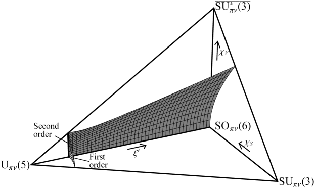
Figure 4: Phase diagram of the proton-neutron interacting boson model (IBM-2) for the $F$-spin invariant Hamiltonian (3.2) with $N_{\pi}=N_{\nu}$, as obtained by numerical minimization of $\mathcal{E}$. The surfaces of first-order and second-order transition between regions of undeformed, axially symmetric deformed, and triaxially deformed equilibria are shown. Only one “quadrant” of parameter space ($0\leq\xi^{\prime}\leq 1$, $-\sqrt{7}/2\leq\chi_{S}\leq 0$, and $0\leq\chi_{V}\leq\sqrt{7}/2$) is included in this plot, since the others may be obtained by reflection. The $\chi_{S}$ and $\chi_{V}$ axes are scaled by $\xi^{\prime}$, so as to converge to a point at the $\mathrm{U}_{\pi\nu}(5)$ limit. Figure from Ref. [12].

We now consider in detail the evolution of the equilibrium energy and coordinates at selected locations throughout the phase diagram. Within the plane $\xi^{\prime}=1$, the boundary curve separating axially symmetric and triaxial equilibria was established in Sec. 3.2. The equilibrium properties along the $\mathrm{SU}_{\pi\nu}(3)$-$\mathrm{SU}_{\pi\nu}^{*}(3)$ transition line are shown in Fig. 5. Several characteristics may be noted. The second derivative of $\mathcal{E}$ with respect to the control parameter ${\chi_{\nu}}$ is discontinuous, as in an Ehrenfest second-order phase transition. The first derivative of one order parameter, $\gamma_{\nu}$, is infinite at the critical point, with an approximately square-root dependence upon the control parameter after this point, as in a Landau second-order phase transition [39]. The first derivative of $\beta_{\nu}$ at this point is, in contrast, discontinous but finite. In the special case of the $\mathrm{SU}_{\pi\nu}(3)$-$\mathrm{SU}_{\pi\nu}^{*}(3)$ line, as already discussed, the two other order parameters $\beta_{\pi}$ and $\gamma_{\pi}$ completely decouple from the transition process, remaining constant throughout.

Figure 5: Evolution of the equilibrium values of (a) $\mathcal{E}$, (b) $\beta_{\nu}$, and (c) $\gamma_{\nu}$ along the line in parameter space between the $\mathrm{SU}_{\pi\nu}(3)$ and $\mathrm{SU}_{\pi\nu}^{*}(3)$ dynamical symmetries ($\chi_{\pi}=-\sqrt{7}/2$, $-\sqrt{7}/2\leq\chi_{\nu}\leq\sqrt{7}/2$), obtained numerically. The dashed line indicates the second-order transition point, $\chi_{\nu}\approx 0.4035$.

In Fig. 6, the equilibrium properties on lines of constant ${\chi_{V}}$ in the plane $\xi^{\prime}=1$, which would appear as horizontal lines across the diagram of Fig. 3, are shown. These lines cross both the prolate-triaxial and triaxial-oblate second-order transition curves. The equilibrium coordinate values for positive ${\chi_{S}}$ are related to those for negative ${\chi_{S}}$ by the transformations of Sec. 3.1. Observe that the order parameters ($\beta_{\pi}$, $\gamma_{\pi}$, $\beta_{\nu}$, and $\gamma_{\nu}$) are coupled in their behavior at the transition points, all simultaneously exhibiting discontinuities in their derivatives at each transition point. In the limiting case ${\chi_{V}}=0$ [Fig. 6(right)], the two points of second order transition at positive and negative ${\chi_{S}}$ converge to a single point at ${\chi_{S}}=0$. The discontinuities in the second derivative of $\mathcal{E}$ with respect to ${\chi_{S}}$ at the two transition points [Fig. 6(left,middle)] combine to form a “cusp” in $\mathcal{E}$. The discontinuity of $\partial\mathcal{E}/\partial\chi$ at $\chi=0$ was noted in the context of the one-fluid IBM by Jolie et al. [40]. Such a discontinuity in the slope of $\mathcal{E}$ would, according to the Ehrenfest criterion, indicate a first-order phase transition. However, the present case provides an example of the great variety of phenomena possible in multi-parameter problems, as is does not naturally fit the one-dimensional Laundau model for a first-order phase transition. The conventional Landau first-order phase transition [39] involves “competition” between two distinct local minima simultantously present in the energy surface, one overtaking the other as global minimum; whereas, in the present example, a single minimum with $\gamma_{\pi}=\gamma_{\nu}=0$ is present for ${\chi_{S}}<0$, a single minimum with $\gamma_{\pi}=\gamma_{\nu}=\pi/3$ is present for ${\chi_{S}}>0$, and a continuous trajectory of minima of arbitary $\gamma(=\gamma_{\pi}=\gamma_{\nu})$, arising from the $\mathrm{SO}_{\pi\nu}(5)$ symmetry of the Hamiltonian, are present for ${\chi_{S}}=0$. This example suggests the need for a comprehensive extension of the classification schemes for single-parameter phase transitions to cover phase transitions with multiple order parameters (see also Ref. [41, Chapter 17]).

Figure 6: Evolution of the equilibrium properties along rays of constant ${\chi_{V}}$ in the $\xi^{\prime}=1$ plane of parameter space, passing from the region of axially symmetric prolate equilibrium to that of axially symmetric oblate equilibrium. Results are shown for the $F$-spin invariant Hamiltonian (3.2) with $N_{\pi}=N_{\nu}$, along the rays of (left) ${\chi_{V}}=0.8$, (center) ${\chi_{V}}=0.4$, and (right) ${\chi_{V}}=0$. Proton fluid variables ($\beta_{\pi}$ and $\gamma_{\pi}$) are represented by solid curves, while neutron fluid variables ($\beta_{\nu}$ and $\gamma_{\nu}$) are represented by dashed curves. The two points of second order phase transition (left, middle), converging towards the single point ${\chi_{S}}=0$ in the limit ${\chi_{V}}=0$ (right), are marked with arrows.

Finally, we consider the transition between spherical and deformed equilibrium configurations. In Sec. 3.3, an upper bound, $\xi^{\prime}_{c}(\chi_{S},\chi_{V})\leq\xi^{\prime}_{c}(\chi_{S},0)$ was placed upon the location of the spherical-deformed transition surface [see Eqn. (3.13)], equality holding in the case $\beta_{\pi}=\beta_{\nu}$. The actual shape of this surface, visible on a coarse scale in Fig. 4, is shown in detail in Fig. 7. Several “vertical” slices through the surface, at constant ${\chi_{S}}$, are plotted. The line of second-order phase transition at $\xi^{\prime}=1/5$ appears rightmost in the figure. The curves vary little in $\xi^{\prime}$ ($\lesssim 0.2\%$) below their upper bound.

Figure 7: Slices through the boundary surface between the regions of spherical and deformed equilibrium at fixed ${\chi_{S}}$. The $\xi^{\prime}$ value at ${\chi_{V}}=0$ is the value $\xi^{\prime}_{c}({\chi_{S}})$ from the one-fluid IBM (3.3), and the recession of each curve towards smaller $\xi^{\prime}$ above ${\chi_{V}}=0$ indicates the extent to which $\xi^{\prime}_{c}({\chi_{S}},{\chi_{V}})$ recedes below the upper limit (3.13) obtained using $\beta_{\pi}=\beta_{\nu}$. The curves shown are for ${\chi_{S}}=0$ to $1$ in steps of $0.1$ (right to left).

The evolution of equilibrium properties across the spherical-deformed transition is shown in Fig. 8. The second-order transition along the $\mathrm{U}_{\pi\nu}(5)$-$\mathrm{SO}_{\pi\nu}(6)$ line and the first-order transition along the $\mathrm{U}_{\pi\nu}(5)$-$\mathrm{SU}_{\pi\nu}(3)$ line, quantitatively identical to the corresponding transitions in the one-fluid IBM, are shown for reference [Fig. 8(left,middle)]. The transition along the $\mathrm{U}_{\pi\nu}(5)$-$\mathrm{SU}_{\pi\nu}^{*}(3)$ line [Fig. 8(right)] is strongly constrained by the proton-neutron interchange symmetry about ${\chi_{S}}=0$, with $\beta_{\pi}=\beta_{\nu}$ and with $\gamma_{\pi}$ and $\gamma_{\nu}$ symmetric to each other about $\pi/6$.

Figure 8: Evolution of the equilibrium properties in the vicinity of the transition between spherical and deformed equilibria. Results are shown for the $F$-spin invariant Hamiltonian (3.2) with $N_{\pi}=N_{\nu}$, along (left) the $\mathrm{U}_{\pi\nu}(5)-\mathrm{SO}_{\pi\nu}(6)$ transition line (${\chi_{S}}=0$, ${\chi_{V}}=0$), (middle) the $\mathrm{U}_{\pi\nu}(5)-\mathrm{SU}_{\pi\nu}(3)$ transition line (${\chi_{S}}=-\sqrt{7}/2$, ${\chi_{V}}=0$), and (right) the $\mathrm{U}_{\pi\nu}(5)-\mathrm{SU}_{\pi\nu}^{*}(3)$ transition line (${\chi_{S}}=0$, ${\chi_{V}}=-\sqrt{7}/2$). Proton fluid variables are represented by solid curves, while neutron fluid variables are represented by dashed curves. Equilibrium $\gamma_{\rho}$ values are undefined, and therefore not shown, when $\beta_{\rho}=0$ (h,i) and along the entire $\mathrm{U}_{\pi\nu}(5)-\mathrm{SO}_{\pi\nu}(6)$ transition line (g). Points of phase transition are marked with arrows.

4 Phase structure for a general Hamiltonian

4.1 Energy surface parameters

In the preceding section, the general features of the IBM-2 phase diagram were established using a schematic Hamiltonian, and only the case $N_{\pi}=N_{\nu}$ was considered. We now address the more general Hamiltonian of Eqn. (2.1) and also consider arbitrary values of the ratio $N_{\pi}/N_{\nu}$. These two generalizations are closely related, as the coefficients in the energy surface $\mathcal{E}$ depend upon the Hamiltonian coefficients and the boson numbers in combination. To make explicit the dependence of each term contributing to $\mathcal{E}$ upon parameters, boson numbers, and coordinates, we express $\mathcal{E}$ as

$$\mathcal{E}=\varepsilon_{\pi}N_{\pi}\,f_{\pi}(\beta_{\pi})+\varepsilon_{\nu}N_{\nu}\,f_{\nu}(\beta_{\nu})+\kappa_{\pi\pi}N_{\pi}^{2}\,f_{\pi\pi}(\chi_{\pi};\beta_{\pi},\gamma_{\pi})\\ +\kappa_{\pi\nu}N_{\pi}N_{\nu}\,f_{\pi\nu}(\chi_{\pi},\chi_{\nu};\beta_{\pi},\gamma_{\pi},\beta_{\nu},\gamma_{\nu},\vartheta_{1},\vartheta_{2},\vartheta_{3})+\kappa_{\nu\nu}N_{\nu}^{2}\,f_{\nu\nu}(\chi_{\nu};\beta_{\nu},\gamma_{\nu})\\ +\lambda N_{\pi}N_{\nu}\,f_{M}(\beta_{\pi},\gamma_{\pi},\beta_{\nu},\gamma_{\nu},\vartheta_{1},\vartheta_{2},\vartheta_{3}).$$ (4.1)

The functions $f$ (e.g., $f_{\pi}\equiv\langle\hat{n}_{d\pi}\rangle/N_{\pi}$) may be read off directly from Eqns. (2.9)–(2.13). The limit of both large $N_{\pi}$ and large $N_{\nu}$ has been taken, so that in $\langle\hat{Q}_{\rho}\cdot\hat{Q}_{\rho}\rangle$ the term linear in $N_{\rho}$ is suppressed. The energy surface (4.1) is entirely determined by the boson-number-weighted coefficients $\varepsilon_{\rho}^{\prime}\equiv\varepsilon_{\rho}N_{\rho}$, $\kappa_{\rho\rho^{\prime}}^{\prime}\equiv\kappa_{\rho\rho^{\prime}}N_{\rho}N_{\rho^{\prime}}$, and $\lambda^{\prime}\equiv\lambda N_{\pi}N_{\nu}$, together with the $\chi_{\rho}$, in terms of which

$$\mathcal{E}=\varepsilon_{\pi}^{\prime}f_{\pi}(\beta_{\pi})+\varepsilon_{\nu}^{\prime}f_{\nu}(\beta_{\nu})+\kappa_{\pi\pi}^{\prime}f_{\pi\pi}(\chi_{\pi};\beta_{\pi},\gamma_{\pi})\\ +\kappa_{\pi\nu}^{\prime}f_{\pi\nu}(\chi_{\pi},\chi_{\nu};\beta_{\pi},\gamma_{\pi},\beta_{\nu},\gamma_{\nu},\vartheta_{1},\vartheta_{2},\vartheta_{3})+\kappa_{\nu\nu}^{\prime}f_{\nu\nu}(\chi_{\nu};\beta_{\nu},\gamma_{\nu})\\ +\lambda^{\prime}f_{M}(\beta_{\pi},\gamma_{\pi},\beta_{\nu},\gamma_{\nu},\vartheta_{1},\vartheta_{2},\vartheta_{3}).$$ (4.2)

4.2 Quadrupole interaction coupling coefficients

The dominant role of the proton-neutron quadrupole interaction in producing collective nuclear deformation has been well established [42]. Consequently, the like-nucleon quadrupole interactions are often neglected in the IBM-2 Hamiltonian (see Refs. [7, 43, 38]). Microsopic estimates suggest that the shell model proton-proton and neutron-neutron quadrupole interactions each have $\sim$1/10 to 1/5 the strength of the proton-neutron quadrupole interaction [44]. However, within the IBM-2, significant further strength is added to the effective like-nucleon interactions by renormalization effects arising from elimination of $g$-wave nucleon pairs from the model space. This may yield like-nucleon coupling strengths comparable to the proton-neutron coupling strength [45]. The actual coupling strengths are a subject for further phenomenological study. Examples spanning a considerable range of values for $\kappa_{\rho\rho}/\kappa_{\pi\nu}$ are included in the following analysis.

For investigation of the phase diagram for the Hamiltonian (2.1), it is convenient to again define a transition parameter $\xi^{\prime}$ controling the relative weights of the $\hat{n}_{d}$ operator and quadrupole operator in the Hamiltonian. This provides a coordinate system for the parameter space like that in Fig. 2. The contributions of the different terms within each of these operators can then be specified by parameters $e^{\prime}_{\rho}$ and $k^{\prime}_{\rho\rho^{\prime}}$ defined such that

$$H=(1-\xi^{\prime})\,\left(\frac{e^{\prime}_{\pi}}{N_{\pi}}\hat{n}_{d\pi}+\frac{e^{\prime}_{\nu}}{N_{\nu}}\hat{n}_{d\nu}\right)\\ \,-\,\xi^{\prime}\,\left(\frac{k^{\prime}_{\pi\pi}}{N_{\pi}^{2}}\hat{Q}_{\pi}^{\chi_{\pi}}\cdot\hat{Q}_{\pi}^{\chi_{\pi}}+\frac{k^{\prime}_{\pi\nu}}{N_{\pi}N_{\nu}}\hat{Q}_{\pi}^{\chi_{\pi}}\cdot\hat{Q}_{\nu}^{\chi_{\nu}}+\frac{k^{\prime}_{\nu\nu}}{N_{\nu}^{2}}\hat{Q}_{\nu}^{\chi_{\nu}}\cdot\hat{Q}_{\nu}^{\chi_{\nu}}\right),$$ (4.3)

yielding a $N_{\rho}$-independent expression

$$\mathcal{E}=(1-\xi^{\prime})\left(e^{\prime}_{\pi}f_{\pi}+e^{\prime}_{\nu}f_{\nu}\right)-\xi^{\prime}\left(k^{\prime}_{\pi\pi}f_{\pi\pi}+k^{\prime}_{\pi\nu}f_{\pi\nu}+k^{\prime}_{\nu\nu}f_{\nu\nu}\right)$$ (4.4)

for the energy surface. To unambiguously define $\xi^{\prime}$ and avoid redundancy in the parameters, we adopt the normalization convention $e^{\prime}_{\pi}+e^{\prime}_{\nu}=1$ and $k^{\prime}_{\pi\pi}+k^{\prime}_{\pi\nu}+k^{\prime}_{\nu\nu}=1$. This choice gives $e^{\prime}_{\rho}=\varepsilon_{\rho}^{\prime}/(\varepsilon_{\pi}^{\prime}+\varepsilon_{\nu}^{\prime})$ and $k^{\prime}_{\rho\rho^{\prime}}=\kappa_{\rho\rho^{\prime}}^{\prime}/(\kappa_{\pi\pi}^{\prime}+\kappa_{\pi\nu}^{\prime}+\kappa_{\nu\nu}^{\prime})$ and is consistent with the definition of $\xi^{\prime}$ in Eqn. (3.2). For the $F$-spin invariant Hamiltonian with arbitrary $N_{\pi}/N_{\nu}$, the parameters are $e^{\prime}_{\pi}=N_{\pi}/N$, $e^{\prime}_{\nu}=N_{\nu}/N$, $k^{\prime}_{\pi\pi}=N_{\pi}^{2}/N^{2}$, $k^{\prime}_{\pi\nu}=2N_{\pi}N_{\nu}/N^{2}$, and $k^{\prime}_{\nu\nu}=N_{\nu}^{2}/N^{2}$.

Analytic results for the phase structure of the Hamiltonian (2.1) with arbitrary quadrupole coupling coefficients can be obtained in the case $\xi^{\prime}=1$ by a straight-forward extension of the analysis described in Sec. 3.2. Surrounding the $\mathrm{SU}_{\pi\nu}(3)$ and $\overline{\mathrm{SU}_{\pi\nu}(3)}$ dynamical symmetries are regions of parameter space in which the equilibrium deformation is axially symmetric ($\gamma_{\pi}=\gamma_{\nu}=0$ or $\pi/3$). The energy surface in this case can be expressed in terms of the function $F$ (of Appendix B) as

$$\mathcal{E}(\beta_{\pi},\beta_{\nu})=4\Bigl{[}\kappa_{\pi\pi}^{\prime}F(-\chi_{\pi}/\sqrt{14};\sigma\beta_{\pi})^{2}\\ +\kappa_{\pi\nu}^{\prime}F(-\chi_{\pi}/\sqrt{14};\sigma\beta_{\pi})F(-\chi_{\nu}/\sqrt{14};\sigma\beta_{\nu})+\kappa_{\nu\nu}^{\prime}F(-\chi_{\nu}/\sqrt{14};\sigma\beta_{\nu})^{2}\Bigr{]},$$ (4.5)

with $\sigma=\cos 3\gamma_{\rho}=\pm 1$. This expression is simply a quadratic form in the quantities $F$, and the extremization problem reduces to a constrained minimization of the quadratic form with respect to these quantities. Since the $\beta_{\rho}$ are limited to positive values, the $F$ are restricted to the rectangular region $0\leq F(-\chi_{\pi}/\sqrt{14};\beta_{\pi})\leq x_{+}(-\chi_{\pi}/\sqrt{14})$ and $0\leq F(-\chi_{\nu}/\sqrt{14};\beta_{\nu})\leq x_{+}(-\chi_{\nu}/\sqrt{14})$ for the case $\sigma=+1$ [$\mathrm{SU}_{\pi\nu}(3)$-like] or to $x_{-}(-\chi_{\pi}/\sqrt{14})\leq F(-\chi_{\pi}/\sqrt{14};-\beta_{\pi})\leq 0$ and $x_{-}(-\chi_{\nu}/\sqrt{14})\leq F(-\chi_{\nu}/\sqrt{14};-\beta_{\nu})\leq 0$ for $\sigma=-1$ [$\overline{\mathrm{SU}_{\pi\nu}(3)}$-like]. Provided $\kappa_{\pi\pi}$, $\kappa_{\pi\nu}$, and $\kappa_{\nu\nu}$ are all negative, the global minimum is again given by Eqn. (3.6) for $\sigma=+1$ or Eqn. (3.7) for $\sigma=-1$. The energy at the minimum is, in terms of the equilibrium $\beta_{\rho}$ values,

$$\mathcal{E}=\kappa_{\pi\pi}^{\prime}\beta_{\pi}^{2}+\kappa_{\pi\nu}^{\prime}\beta_{\pi}\beta_{\nu}+\kappa_{\nu\nu}^{\prime}\beta_{\nu}^{2}.$$ (4.6)

The boundary curve separating axial and triaxial deformations is found as in Sec. 3.2 from analysis of the second derivatives of $\mathcal{E}$. The axial minimum becomes unstable with respect to $\gamma$ deformation along a curve in parameter space, again most conveniently expressed in terms of the equilibrium $\beta_{\rho}$ values, given by

$$1=\frac{18\frac{\kappa_{\pi\pi}^{\prime}}{\kappa_{\pi\nu}^{\prime}}\beta_{\pi}(\beta_{\pi}^{2}-1)+\beta_{\nu}(2\beta_{\pi}^{2}-1)(\beta_{\pi}^{2}+1)}{2\beta_{\pi}(\beta_{\pi}^{2}-2)^{2}}\\ \times\frac{18\frac{\kappa_{\nu\nu}^{\prime}}{\kappa_{\pi\nu}^{\prime}}\beta_{\nu}(\beta_{\nu}^{2}-1)+\beta_{\pi}(2\beta_{\nu}^{2}-1)(\beta_{\nu}^{2}+1)}{2\beta_{\nu}(\beta_{\nu}^{2}-2)^{2}}.$$ (4.7)

The instability occurs against deformations with a ratio $\gamma_{\pi}/\gamma_{\nu}$ given by Eqn. (3.10) with the values

$$A \equiv 9\kappa_{\pi\pi}^{\prime}\beta_{\pi}^{2}(\beta_{\pi}^{2}-1)+\beta_{\pi}\beta_{\nu}(2\beta_{\pi}^{2}-1)(\beta_{\pi}^{2}+1)$$ (4.8)

$$B \equiv-2\kappa_{\pi\nu}^{\prime}\beta_{\pi}\beta_{\nu}(\beta\pi^{2}-2)(\beta_{\nu}^{2}-2)$$

$$C \equiv 9\kappa_{\nu\nu}^{\prime}\beta_{\nu}^{2}(\beta_{\nu}^{2}-1)+\beta_{\pi}\beta_{\nu}(2\beta_{\nu}^{2}-1)(\beta_{\nu}^{2}+1).$$

Along the $\mathrm{SU}_{\pi\nu}(3)$-$\mathrm{SU}_{\pi\nu}^{*}(3)$ line in parameter space, the location of the phase transition is obtained by solution of the quartic equation

$$18\frac{\kappa_{\nu\nu}^{\prime}}{\kappa_{\pi\nu}^{\prime}}\beta_{\nu}(\beta_{\nu}^{2}-1)+\sqrt{2}(2\beta_{\nu}^{2}-1)(\beta_{\nu}^{2}+1)=0,$$ (4.9)

and a similar relation with interchanged proton and neutron labels holds for the $\mathrm{SU}_{\pi\nu}(3)$-$\overline{\mathrm{SU}_{\pi\nu}^{*}(3)}$ line. Observe that the $\chi_{\nu}$ value at which the transition occurs depends only upon the ratio $\kappa_{\nu\nu}^{\prime}/\kappa_{\pi\nu}^{\prime}$.

The dependence of the second-order transition curve upon $N_{\pi}/N_{\nu}$ is illustrated in Fig. 9. Since $\kappa_{\pi\pi}^{\prime}\neq\kappa_{\nu\nu}^{\prime}$, the phase diagram is not symmetric under reflection with respect to ${\chi_{S}}$ or ${\chi_{V}}$ but remains symmetric under inversion (3.4). It is seen that increasing $N_{\pi}/N_{\nu}$ from unity moves the $\mathrm{SU}_{\pi\nu}(3)$-$\mathrm{SU}_{\pi\nu}^{*}(3)$ transition farther away in parameter space from $\mathrm{SU}_{\pi\nu}(3)$ while moving the $\mathrm{SU}_{\pi\nu}(3)$-$\overline{\mathrm{SU}_{\pi\nu}^{*}(3)}$ transition closer. The $N_{\pi}/N_{\nu}$ depencence of the boundary curve raises the possibility of considering phase transitions at a fixed point in the Hamiltonian parameter space with $N_{\pi}/N_{\nu}$ as the control parameter, i.e., phase transitions as a function of particle number.

Figure 9: The curve of second-order phase transition between axial and triaxial deformation in the plane $\xi^{\prime}=1$, shown for the $F$-spin invariant Hamiltonian with different boson number ratios $N_{\pi}/N_{\nu}$: (a) $N_{\pi}/N_{\nu}=2$ and (b) $N_{\pi}/N_{\nu}=4$. The boundary curve for $N_{\pi}/N_{\nu}=1$ (Fig. 3) is shown in each panel (dashed curve) for comparison.

For the $F$-spin invariant Hamiltonian considered in Sec. 3, the transition between prolate axially symmetric equilibrium [$\mathrm{SU}_{\pi\nu}(3)$-like] and oblate axially symmetric equilibrium [$\overline{\mathrm{SU}_{\pi\nu}(3)}$-like] always proceeds through an intermediate stage of triaxial equilibrium, except at the point in parameter space corresponding to $\mathrm{SO}_{\pi\nu}(6)$. However, if $\kappa_{\pi\pi}^{\prime}$ and $\kappa_{\nu\nu}^{\prime}$ are sufficiently small relative to $\kappa_{\pi\nu}^{\prime}$, it is possible for a direct transition to occur between the prolate and oblate equilibria of Eqns. (3.6) and (3.7) without either minimum becoming unstable with respect to triaxiality and thus for the regions of prolate and oblate equilibrium in the phase diagram to share a common boundary. The boundary curve is given by

$$\kappa_{\pi\pi}^{\prime 2}a_{\pi}^{2}(a_{\pi}^{2}+1)-\kappa_{\nu\nu}^{\prime 2}a_{\nu}^{2}(a_{\nu}^{2}+1)+\kappa_{\pi\nu}^{\prime}\kappa_{\pi\pi}^{\prime}a_{\pi}a_{\nu}(a_{\pi}^{2}+1)\\ -\kappa_{\pi\nu}^{\prime}\kappa_{\nu\nu}^{\prime}a_{\pi}a_{\nu}(a_{\nu}^{2}+1)-\frac{1}{4}\kappa_{\pi\nu}^{\prime 2}(a_{\pi}^{2}-a_{\nu}^{2})=0,$$ (4.10)

where $a_{\rho}\equiv-{\chi_{\rho}}/\sqrt{14}$. Over the range of ${\chi_{\rho}}$ and parameter values considered, this curve differs little from its small-${\chi_{\rho}}$ approximation, the line ${\chi_{S}}/{\chi_{V}}=-(\kappa_{\pi\pi}^{\prime}-\kappa_{\nu\nu}^{\prime})/(\kappa_{\pi\pi}^{\prime}+\kappa_{\pi\nu}^{\prime}+\kappa_{\nu\nu}^{\prime})$. For any proton-neutron symmetric energy surface ($\kappa_{\pi\pi}^{\prime}=\kappa_{\nu\nu}^{\prime}$), the boundary curve (4.10) reduces to the line ${\chi_{S}}=0$. The general problem of determining whether or not the prolate and oblate regions of the phase diagram share a common boundary involves solving for an intersection of the curves (4.7) and (4.10). For the proton-neutron symmetric case ($\kappa_{\pi\pi}^{\prime}=\kappa_{\nu\nu}^{\prime}$), a prolate-oblate boundary arises for $\kappa_{\rho\rho}^{\prime}/\kappa_{\pi\nu}^{\prime}\leq(\sqrt{13}-2)/18\approx 0.08919$.

The dependence of the boundary curve upon the relative strengths of like-nucleon and proton-neutron quadrupole coupling coefficients is shown in Fig. 10. As the $\kappa_{\rho\rho}^{\prime}$ are reduced in strength relative to $\kappa_{\pi\nu}^{\prime}$, the region of triaxial equilibrium contracts. Its separation from the origin and the onset of a direct prolate-oblate transition for $\kappa_{\rho\rho}^{\prime}/\kappa_{\pi\nu}^{\prime}\leq(\sqrt{13}-2)/18$ is illustrated in Fig. 10(b). The parameter values chosen for Fig. 9(a) and for Fig. 10(a) are such that $\kappa_{\nu\nu}^{\prime}/\kappa_{\pi\nu}^{\prime}$ is the same ($\kappa_{\nu\nu}^{\prime}/\kappa_{\pi\nu}^{\prime}=1/4$) in both cases. Thus, though the curves in these two figures are quite different overall, by Eqn. (4.9) they share the same endpoint ($\chi_{\nu}\approx 0.6177$) on the $\mathrm{SU}_{\pi\nu}(3)$-$\mathrm{SU}_{\pi\nu}^{*}(3)$ line. Numerical results for the equilibrium values of the energy and coordinates along the $\mathrm{SU}_{\pi\nu}(3)$-$\mathrm{SU}_{\pi\nu}^{*}(3)$ line for different relative strengths of like-nucleon and proton-neutron quadrupole interactions are shown in Fig. 11. Although the transition to triaxial equilibrium is progressively delayed as $\kappa_{\nu\nu}^{\prime}/\kappa_{\pi\nu}^{\prime}$ decreases, the triaxial configuration of Fig. 1, with orthogonal symmetry axes ($\gamma_{\pi}=0$, $\gamma_{\nu}=\pi/3$), is still ultimately achieved in the $\mathrm{SU}_{\pi\nu}^{*}(3)$ limit.

Figure 10: The curve of second-order phase transition between axial and triaxial deformation in the plane $\xi^{\prime}=1$, shown for different relative strengths of like-nucleon and proton-neutron quadrupole interactions: (a) $\kappa_{\pi\pi}/\kappa_{\pi\nu}=\kappa_{\nu\nu}/\kappa_{\pi\nu}=1/4$ and (b) $\kappa_{\pi\pi}/\kappa_{\pi\nu}=\kappa_{\nu\nu}/\kappa_{\pi\nu}=1/12$. Both curves are for $N_{\pi}=N_{\nu}$. The boundary curve for $\kappa_{\pi\pi}/\kappa_{\pi\nu}=\kappa_{\nu\nu}/\kappa_{\pi\nu}=1/2$ (Fig. 3) is shown in each panel (dashed curve) for comparison.

Figure 11: Evolution of the equilibrium properties between the $\mathrm{SU}_{\pi\nu}(3)$ and $\mathrm{SU}_{\pi\nu}^{*}(3)$ dynamical symmetries, for different relative strengths of like-nucleon and proton-neutron quadrupole interactions: (left) $\kappa_{\pi\pi}/\kappa_{\pi\nu}=\kappa_{\nu\nu}/\kappa_{\pi\nu}=1/2$ (for reference), (middle) $\kappa_{\pi\pi}/\kappa_{\pi\nu}=\kappa_{\nu\nu}/\kappa_{\pi\nu}=1/4$ and (right) $\kappa_{\pi\pi}/\kappa_{\pi\nu}=\kappa_{\nu\nu}/\kappa_{\pi\nu}=1/12$. The curves are for $N_{\pi}=N_{\nu}$. Proton fluid variables are represented by solid curves, while neutron fluid variables are represented by dashed curves. Points of phase transition are marked with arrows.

A qualitative understanding of the mechanism underlying the parameter dependences observed in Figs. 9 and 10 is easily obtained. Among the quadrupole terms in the energy surface, the $\langle\hat{Q}_{\pi}\cdot\hat{Q}_{\pi}\rangle$ term has a dominant influence on the proton fluid equilibrium deformation, the $\langle\hat{Q}_{\nu}\cdot\hat{Q}_{\nu}\rangle$ terms drives the neutron fluid deformation, and the $\langle\hat{Q}_{\pi}\cdot\hat{Q}_{\nu}\rangle$ term couples the two deformations. The $\mathrm{SU}_{\pi\nu}^{*}(3)$ configuration with orthogonal symmetry axes (Fig. 1) arises since the $\langle\hat{Q}_{\pi}\cdot\hat{Q}_{\pi}\rangle$ term stabilizes the proton fluid about a prolate deformation and the $\langle\hat{Q}_{\nu}\cdot\hat{Q}_{\nu}\rangle$ term stabilizes the neutron fluid about an oblate deformation, while the $\langle\hat{Q}_{\pi}\cdot\hat{Q}_{\nu}\rangle$ term is responsible for the relative orientation of the symmetry axes. All three terms are essential to producing the $\mathrm{SU}_{\pi\nu}^{*}(3)$ triaxial equilibrium configuration. If the strengths of the like-nucleon quadrupole interactions are both reduced relative to that of the proton-neutron interaction (Figs. 10 and 11), the ability of the like-nucleon terms to stabilize the proton and neutron fluids about distinct deformations is reduced, against the tendency of the proton-neutron term to favor equal deformations. The onset of triaxiality is thus delayed. For $N_{\pi}/N_{\nu}$ greater than unity (Fig. 9), the relative weight of the $\langle\hat{Q}_{\pi}\cdot\hat{Q}_{\pi}\rangle$ contribution to $\mathcal{E}$ increases, while that of the $\langle\hat{Q}_{\nu}\cdot\hat{Q}_{\nu}\rangle$ contribution decreases. Thus, a larger larger positive $\chi_{\nu}$ (oblate tendency for the neutron fluid) is needed for the neutrons to undergo a transition to an oblate configuration against the restraining influence of the protons, while only a small positive $\chi_{\pi}$ (oblate tendency for the proton fluid) is necessary for the protons to undergo a transition to an oblate configuration.

Limited analytic results can also be obtained for the transition between spherical and deformed equilibrium. Consider the stability of the minimum at $\beta_{\pi}=\beta_{\nu}=0$. The second derivative of $\mathcal{E}$ along the ray $\beta_{\pi}=u_{\pi}\beta$ and $\beta_{\nu}=u_{\nu}\beta$ is

$$\left.\frac{d^{2}\mathcal{E}}{d\beta^{2}}\right|_{\beta=0}=2u_{\pi}^{2}[e^{\prime}_{\pi}(1-\xi^{\prime})-4k^{\prime}_{\pi\pi}\xi^{\prime}]\\ +2u_{\nu}^{2}[e^{\prime}_{\nu}(1-\xi^{\prime})-4k^{\prime}_{\nu\nu}\xi^{\prime}]-8u_{\pi}u_{\nu}k^{\prime}_{\pi\nu}\xi^{\prime}\cos(\gamma_{\pi}-\gamma_{\nu}).$$ (4.11)

As in the special case considered in Sec. 3.3, this quantity is independent of $\chi_{S}$ and $\chi_{V}$ and depends upon the $\gamma_{\rho}$ coordinates only through their difference $\gamma_{\pi}-\gamma_{\nu}$. As $\xi^{\prime}$ is increased from 0, vanishing of this second derivative for some value of $u_{\pi}/u_{\nu}$ and $\gamma_{\pi}-\gamma_{\nu}$ indicates the onset of instability. Since the coefficient of $\cos(\gamma_{\pi}-\gamma_{\nu})$ is negative, instability must first occur for $\gamma_{\pi}-\gamma_{\nu}=0$. With $\gamma_{\pi}-\gamma_{\nu}$ set to zero, $\partial^{2}\mathcal{E}/\partial\beta^{2}|_{\beta=0}$ vanishes at

$$\xi^{\prime}=\frac{e^{\prime}_{\pi}u_{\pi}^{2}+e^{\prime}_{\nu}u_{\nu}^{2}}{(e^{\prime}_{\pi}u_{\pi}^{2}+e^{\prime}_{\nu}u_{\nu}^{2})+4(k^{\prime}_{\pi\pi}u_{\pi}^{2}+k^{\prime}_{\pi\nu}u_{\pi}u_{\nu}+k^{\prime}_{\nu\nu}u_{\nu}^{2})}.$$ (4.12)

Instability against deformations with equal $\beta_{\pi}$ and $\beta_{\nu}$ therefore occurs at $\xi^{\prime}=1/5$ for any values of the energy surface parameters. However, the minimum at $\beta=0$ can in general become unstable against deformations with unequal $\beta_{\pi}$ and $\beta_{\nu}$ at a smaller value of $\xi^{\prime}$. The direction in $(\beta_{\pi},\beta_{\nu})$ space in which instability first sets in is given by a quadratic equation for $u_{\pi}/u_{\nu}$,

$$e^{\prime}_{\nu}k^{\prime}_{\pi\nu}+2(e^{\prime}_{\nu}k^{\prime}_{\pi\pi}-e^{\prime}_{\pi}k^{\prime}_{\nu\nu})\left(\frac{u_{\pi}}{u_{\nu}}\right)-e^{\prime}_{\pi}k^{\prime}_{\pi\nu}\left(\frac{u_{\pi}}{u_{\nu}}\right)^{2}=0.$$ (4.13)

The $\xi^{\prime}$ value at which instability occurs follows from this $u_{\pi}/u_{\nu}$ value by Eqn. (4.12). There are two important special cases in which instability first occurs at $\xi^{\prime}=1/5$: (1) for the $F$-spin invariant Hamiltonian (3.2) with arbitrary $N_{\pi}/N_{\nu}$, and (2) for energy surface parameters which are proton-neutron symmetric (i.e., $\varepsilon_{\pi}^{\prime}=\varepsilon_{\nu}^{\prime}$ and $\kappa_{\pi\pi}^{\prime}=\kappa_{\nu\nu}^{\prime}$), as are obtained whenever a proton-neutron symmetric Hamiltonian is considered with $N_{\pi}=N_{\nu}$.

The evolution of equilibrium properties across the $\mathrm{U}_{\pi\nu}(5)$-$\mathrm{SO}_{\pi\nu}(6)$ second-order transition point for a case asymmetric in $\beta_{\pi}$ and $\beta_{\nu}$ is shown in Fig. 12. From Eqns. (4.12) and (4.13), the phase transition for the parameter values used in the figure ($\varepsilon_{\pi}=\varepsilon_{\nu}$, $\kappa_{\pi\pi}=\kappa_{\nu\nu}=\kappa_{\pi\nu}/4$, and $N_{\pi}/N_{\nu}=4$) occurs at $\xi^{\prime}\approx 0.1959$, with $\beta_{\pi}/\beta_{\nu}\approx 0.7215$. The evolution of the ratio $\beta_{\pi}/\beta_{\nu}$ past this point is shown in Fig. 12(c). Observe that the proton and neutron equilibrium properties in this example are unequal even within the plane ${\chi_{V}}=0$, unlike the case of Sec. 3.1, illustrating that the the IBM-2 equilibrium problem in the general proton-neutron asymmetric case does not reduce to the one-fluid IBM problem.

Figure 12: Evolution of the equilibrium properties along the $\mathrm{U}_{\pi\nu}(5)$-$\mathrm{SO}_{\pi\nu}(6)$ line in parameter space, illustrating instability against deformation with unequal $\beta_{\pi}$ and $\beta_{\nu}$. Results are shown for the Hamiltonian (4.3) with $\varepsilon_{\pi}=\varepsilon_{\nu}$ and $\kappa_{\pi\pi}=\kappa_{\nu\nu}=\kappa_{\pi\nu}/4$ for (left) the symmetric case $N_{\pi}/N_{\nu}=1$ and (right) the asymmetric case $N_{\pi}/N_{\nu}=4$. The variable $\beta_{\pi}$ is represented by the solid curve, while $\beta_{\nu}$ is represented by the dashed curve. The point of phase transition is marked with an arrow.

The minimum at zero deformation always becomes unstable at the $\xi^{\prime}$ value determined by Eqns. (4.12) and (4.13), independent of ${\chi_{S}}$ and ${\chi_{V}}$. However, this gives rise to a second order phase transition only if a first-order transition to a distinct minimum has not already occured at smaller $\xi^{\prime}$ for those values of ${\chi_{S}}$ and ${\chi_{V}}$, as discussed in Sec. 3.3. For the $F$-spin invariant Hamiltonian (3.2) with arbitrary $N_{\pi}/N_{\nu}$, an extension of relation (3.12) is readily found, namely that $\mathcal{E}(\xi^{\prime},\chi_{S},\chi_{V};\beta,0,\beta,0)$ is invariant along any line of constant $N_{\pi}{\chi_{\pi}}+N_{\nu}{\chi_{\nu}}$. By arguments analogous to those of Sec. 3.3, a line of second order phase transition occurs for $\xi^{\prime}=1/5$ and ${\chi_{\pi}}/{\chi_{\nu}}=-N_{\nu}/N_{\pi}$, embedded in a surface of first order phase transition. For a Hamiltonian with arbitrary coupling constants, however, no such simple result is obtained. The full phase diagram of the IBM-2 Hamiltonian (4.3) for a set of parameters involving proton-neutron symmetric couplings ($\kappa_{\pi\pi}/\kappa_{\pi\nu}=\kappa_{\nu\nu}/\kappa_{\pi\nu}=1/4$) but unequal boson numbers ($N_{\pi}/N_{\nu}=4$), obtained by numerical mimimization, is shown in Fig. 13.

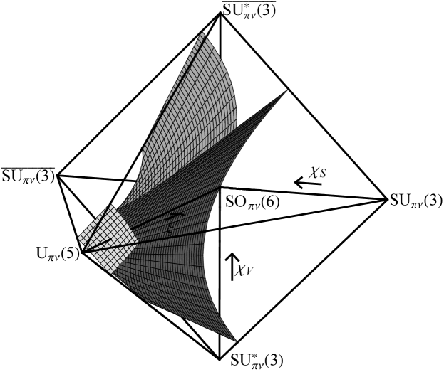
Figure 13: Phase diagram of the IBM-2 for the Hamiltonian (4.3), with $\kappa_{\pi\pi}/\kappa_{\pi\nu}=\kappa_{\nu\nu}/\kappa_{\pi\nu}=1/4$ and $N_{\pi}/N_{\nu}=4$, as obtained by numerical minimization of $\mathcal{E}$. The surfaces of first-order and second-order transition between regions of undeformed, axially symmetric deformed, and triaxially deformed equilibria are shown. The axes are defined as in Fig. 2.

4.3 Majorana operator

The Majorana operator $\hat{M}$ is the analogue in the IBM-2 Hamiltonian to the proton-neutron symmetry energy of the liquid drop model. This operator arises through a combination of direct shell model effects and renormalization effects [46, 47]. As is evident from Eqn. (2.13), this operator energetically discourages configurations with $\beta_{\pi}\neq\beta_{\nu}$ or $\gamma_{\pi}\neq\gamma_{\nu}$. The approximate strength of the Majorana contribution can be deduced from the energies of mixed symmetry excitations [48], including the scissors mode excitation in axial rotor nuclei (e.g., Ref. [49]). Comparison of the $\beta$-vibrational or $\gamma$-vibrational energy scale ($\sim$1 MeV) with the scissors mode energy scale ($\sim$2.5 MeV) indicates $\lambda/\lvert\kappa_{\pi\nu}\rvert\approx 5$ to be a generally reasonable estimate.

For axially symmetric configurations, the contribution of the Majorana operator to the energy surface is, from Eqn. (2.13), $\langle\hat{M}\rangle=N_{\pi}N_{\nu}(1+\beta_{\pi}^{2})^{-1}(1+\beta_{\nu}^{2})^{-1}(\beta_{\pi}-\beta_{\nu})^{2}$. If the equilibrium configuration without the Majorana operator already has $\beta_{\pi}=\beta_{\nu}$, as in the ${\chi_{S}}=0$ plane for the proton-neutron symmetric case of Fig. 2, then introduction of the Majorana term has no further effect. Otherwise, the effect of the Majorana contribution is, naturally, to bring the equilibrium values $\beta_{\pi}$ and $\beta_{\nu}$ closer to each other. In the plane $\xi^{\prime}=1$, this invalidates the simple results (3.6) and (3.7) giving the equilibrium $\beta_{\pi}$ purely as a function of ${\chi_{\pi}}$ and the equilibrium $\beta_{\nu}$ as a function of ${\chi_{\nu}}$. The derivation of the simple equations (3.9) and (4.7) for the curve on which the axial minimum becomes unstable with respect to the $\gamma_{\rho}$ depended upon the use of these results to eliminate ${\chi_{\rho}}$ in favor of $\beta_{\rho}$ at the minimum, a simplification which is no longer possible with a Majorana contribution.

Investigation of the equilibrium properties in the presence of a Majorana operator must therefore rely upon numerical minimization. The evolution of the equilibrium properties between the $\mathrm{SU}_{\pi\nu}(3)$ and $\mathrm{SU}_{\pi\nu}^{*}(3)$ points in parameter space, for different strengths of the Majorana term in the Hamiltonian, is shown in Fig. 14. The Majorana operator is seen to have two main effects on the transition to triaxial equilibrium. The triaxial configuration of Fig. 1 is highly proton-neutron asymmetric, and thus penalized energetically by the Majorana operator, as seen from Eqn. (2.13). Thus, first, the transition to towards such triaxial structure is delayed by the Majorana operator. Second, the Majorana operator has the effect of bringing the proton and neutron coordinate values closer together throughout the transition. The $\mathrm{SU}_{\pi\nu}(3)$-$\mathrm{SU}_{\pi\nu}^{*}(3)$ line is an extreme case. Without the Majorana operator [Fig. 5 or 14(a)], the evolution of the proton coordinates is completely decoupled from that of the neutron coordinates, and their equilibrium values are constant along the line. A Majorana strength of $\lambda/\kappa_{\pi\nu}\approx 10$ is sufficent, however, to cause the two fluids’ $\beta_{\rho}$ and $\gamma_{\rho}$ coordinates to remain nearly equal throughout the evolution. The triaxial configurations produced are thus essentially one-fluid, like those described by the Davydov model [50] or by the one-fluid IBM with three-body or four-body operators in the Hamiltonian [26, 28, 51, 52, 53]. As the Majorana strength increases, the global minimum at triaxial deformation becomes very shallow, and the difference in energy between the $\gamma_{\pi}\approx\gamma_{\nu}\approx\pi/6$ triaxial minimum and axial deformations ($\gamma_{\pi}=\gamma_{\nu}=0$) approaches zero, as shown in Fig. 15. This indicates that the equilibrium structure for large Majorana strengths is essentially one-fluid $\gamma$-unstable, or $\mathrm{SO}(6)$-like, rather than rigidly triaxial.

Figure 14: Evolution of the equilibrium properties between the $\mathrm{SU}_{\pi\nu}(3)$ and $\mathrm{SU}_{\pi\nu}^{*}(3)$ dynamical symmetries, for different Majorana operator strengths: (left) $\lambda/\kappa_{\pi\nu}=0$ (for reference), (middle) $\lambda/\kappa_{\pi\nu}=1$, and (right) $\lambda/\kappa_{\pi\nu}=10$. The curves are for the quadrupole coefficient values $\kappa_{\pi\pi}/\kappa_{\pi\nu}=\kappa_{\nu\nu}/\kappa_{\pi\nu}=1/2$ with $N_{\pi}=N_{\nu}$. Proton fluid variables are represented by solid curves, while neutron fluid variables are represented by dashed curves. Points of phase transition are marked with arrows.

Figure 15: Global minimum energy (solid curve) and the lowest energy for axial ($\gamma_{\pi}=\gamma_{\nu}=0$) deformations (dashed curve), shown as a function of $\lambda/\kappa_{\pi\nu}$, at the $\mathrm{SU}_{\pi\nu}^{*}(3)$ point in parameter space. The difference is a measure of the $\gamma$-stiffness of the triaxial minimum. The curves are for quadrupole coefficient values $\kappa_{\pi\pi}/\kappa_{\pi\nu}=\kappa_{\nu\nu}/\kappa_{\pi\nu}=1/2$ with $N_{\pi}=N_{\nu}$.

The decomposition of the Majorana operator into multipole components, easily obtained from Ref. [21, (A2)], includes a nonzero hexadecapole contribution. The analysis of Ref. [21] therefore allows the existence of “oblique” equilibrium configurations, in which the proton and neutron intrinsic frames are not aligned. For axially symmetric aligned configurations ($\vartheta_{i}$ and $\gamma_{\rho}$ all vanishing), instability with respect to the Euler angles is simple to investigate. The Hessian matrix of $\mathcal{E}$ with respect to the coordinates $\beta_{\pi}$, $\beta_{\nu}$, $\gamma_{\pi}$, $\gamma_{\nu}$, and $\vartheta_{2}$ decomposes as a direct sum $\mathcal{H}=\mathcal{H}_{\beta}\oplus\mathcal{H}_{\gamma}\oplus\mathcal{H}_{\vartheta_{2}}$, with $\mathcal{H}_{\beta}$ involving only derivatives with respect to the $\beta_{\rho}$, etc.. The dependence upon the azimuthal Euler angles $\vartheta_{1}$ and $\vartheta_{3}$ vanishes by axial symmetry. Thus, instability would be indicated simply by a negative second derivative of $\mathcal{E}$ with respect to the opening angle $\vartheta_{2}$ between the proton and neutron frames. For the parameter ranges considered ($\kappa_{\pi\nu}^{\prime}<0$, $\lambda^{\prime}\geq 0$, $\lvert{\chi_{\rho}}\rvert\leq\sqrt{7}/2$) and coordinate values encountered ($\beta_{\rho}\lesssim\sqrt{2}$) in the present study, this quantity is always positive. The possibility of a first order transition to a distinct minimum with nonzero Euler angles must also be considered. Numerical searches provide no evidence for a such a transition, but such searches are necessarily not exhaustive due to the large number of parameters involved.

5 Spectroscopic properties

5.1 Basic properties

To provide a connection between the IBM-2 phase structure considered so far and observable quantities, let us now consider the evolution of the predicted spectroscopic properties — eigenvalues and electromagnetic transition strengths — across the phase transitions. The present discussion emphasises the gross spectroscopic features which emerge in the transitions between the different regions of the phase diagram of Fig. 4. Numerical studies of several observables in the vicinity of the $\mathrm{SU}_{\pi\nu}^{*}(3)$ dynamical symmetry may also be found in Refs. [18, 19].

Electric quadrupole and magnetic dipole transition matrix elements are calculated using transition operators [3]

$$T^{(E2)} =e_{\pi}\hat{Q}_{\pi}^{\chi_{\pi}^{(E2)}}+e_{\nu}\hat{Q}_{\nu}^{\chi_{\nu}^{(E2)}}$$ (5.1)

and

$$T^{(M1)} =\sqrt{\frac{3}{4\pi}}\bigl{[}g_{\pi}\hat{L}_{\pi}+g_{\nu}\hat{L}_{\nu}\bigr{]},$$ (5.2)

where $\hat{L}_{\rho}\equiv\sqrt{10}(d_{\rho}^{{\dagger}}\times\tilde{d}_{\rho})^{(1)}$. The transition strengths are $B(\sigma\lambda;J_{i}\rightarrow J_{f})\equiv(2J_{f}+1)\,|\langle f||T^{(\sigma\lambda)}||i\rangle|^{2}/(2J_{i}+1)$. Schematic values $e_{\pi}=e_{\nu}=0.1\,e\mathrm{b}$, $g_{\pi}=\mu_{N}$, and $g_{\nu}=0$ are used for the effective charges (see Ref. [9] for further discussion). The ${\chi_{\rho}}^{(E2)}$ parameters are taken equal to their counterparts ${\chi_{\rho}}$ in the Hamiltonian, following the consistent quadrupole formalism [54]. The Hamiltonian used for the present discussion is the simple form (3.2) with the addition of the Majorana operator. Diagonalization is carried out using the computer code npbos [55], for boson numbers $N_{\pi}=N_{\nu}=5$.

The energy spectrum for the $\mathrm{SU}_{\pi\nu}^{*}(3)$ symmetry is known analytically [10, 17]. The operator $(\hat{Q}_{\pi}^{\chi_{\pi}}+\hat{Q}_{\nu}^{\chi_{\nu}})\cdot(\hat{Q}_{\pi}^{\chi_{\pi}}+\hat{Q}_{\nu}^{\chi_{\nu}})$ with ${\chi_{\pi}}=-\sqrt{7}/2$ and ${\chi_{\nu}}=+\sqrt{7}/2$ can be reexpressed in terms of the quadratic Casimir operators [3] of the subalgebra chain (2.5), as $(3/4)C_{2}[\mathrm{SU}_{\pi\nu}^{*}(3)]-(3/16)C_{2}[\mathrm{SO}_{\pi\nu}(3)]$. For $H=-\hat{Q}\cdot\hat{Q}$, the eigenvalues are thus given by

$$E(\lambda,\mu,L)=-\frac{1}{2}(\lambda^{2}+\mu^{2}+\lambda\mu+3\lambda+3\mu)+\frac{3}{8}L(L+1),$$ (5.3)

where $(\lambda,\mu)$ are the $\mathrm{SU}_{\pi\nu}^{*}(3)$ Elliott quantum numbers [56] and $L$ is the angular momentum quantum number. This is the $\mathrm{SU}(3)$ energy formula, and level energies within an $\mathrm{SU}_{\pi\nu}^{*}(3)$ representation follow $L(L+1)$ rotational spacings. However, the allowed $\mathrm{SU}(3)$ representations (see Refs. [10, 17]) are different from those for $\mathrm{SU}_{\pi\nu}(3)$. The ground state representation is the $(2N_{\pi},2N_{\nu})$ representation, rather than the usual $\mathrm{SU}_{\pi\nu}(3)$ ground state representation $(2N_{\pi}+2N_{\nu},0)$. According to the $\mathrm{SU}(3)\supset\mathrm{SO}(3)$ branching rules [56], the ground state representation thus contains multiple degenerate rotational bands, with $K$ quantum numbers $0$, $2$, $4$, $\ldots$, as shown in Fig. 16. [It has become customary to label the bands of an $\mathrm{SU}(3)$ representation by the Elliott $K$ quantum number [56], in part by analogy with the rigid rotor spin-projection quantum number $K$ [35], which yields a band of the same band head spin. However, the Elliott $\mathrm{SU}(3)$ basis is not orthogonal, and the orthonormal states obtained from diagonalization of a Hamiltonian are thus not in general Elliott states. Throughout this article, the label $K$ is used simply to indicate the spin content of a band.] Other $\mathrm{SU}_{\pi\nu}^{*}(3)$ representations appearing at low energy include the $(2N_{\pi}-4,2N_{\nu}+2)$, $(2N_{\pi}+2,2N_{\nu}-4)$, and $(2N_{\pi}-1,2N_{\nu}-1)$ representations (Fig. 16). In the classical limit, the first two of these correspond to coupled $\beta$ and $\gamma$ vibrations of the fluids [20]. The last corresponds to an “orthogonal” scissors mode, in which the proton and neutron symmetry axes oscillate about their equilibrium perpendicular relative orientation [20, 17].

Figure 16: Level scheme for the $\mathrm{SU}_{\pi\nu}^{*}(3)$ dynamical symmetry, following the energy relation (5.3). The lowest-energy $\mathrm{SU}_{\pi\nu}^{*}(3)$ representations, labeled by the $(\lambda,\mu)$ quantum numbers, are shown for $N_{\pi}=N_{\nu}=5$.

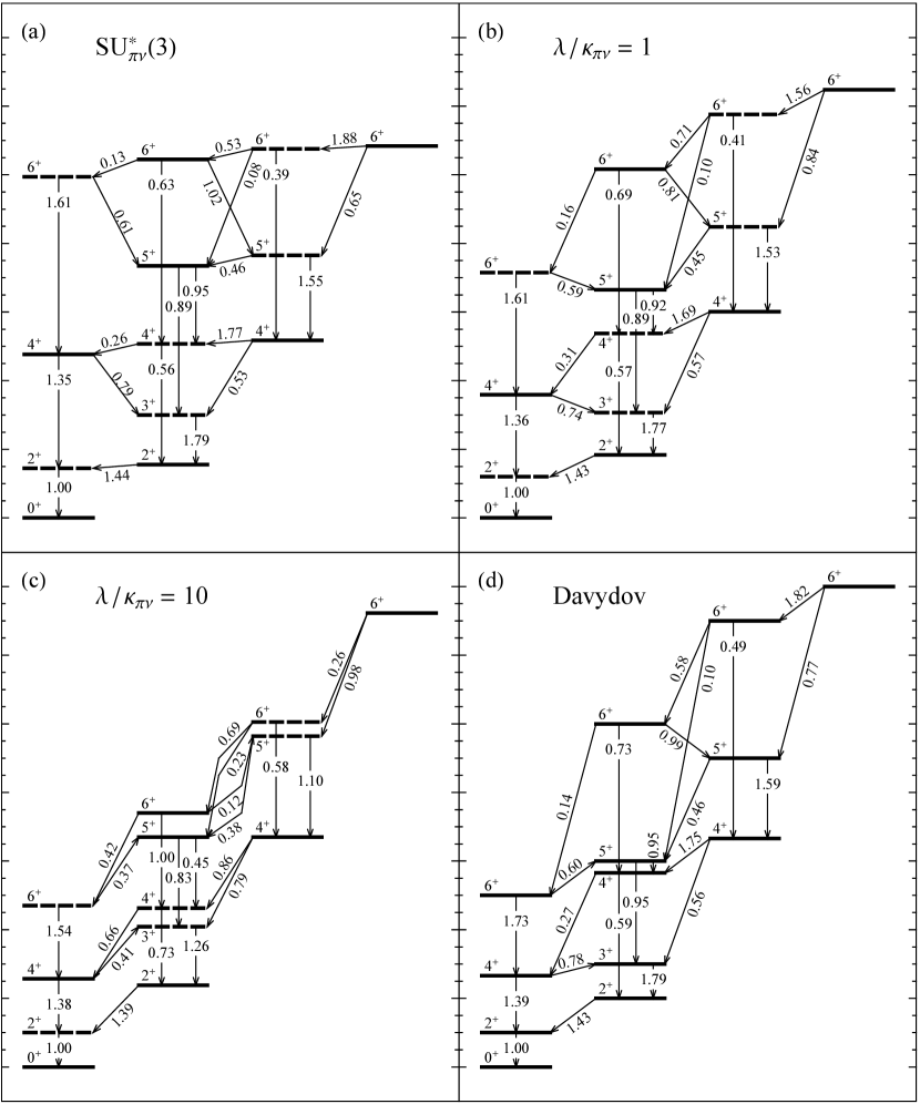
Figure 17: Level schemes and selected $B(E2)$ strengths for (a) the $\mathrm{SU}_{\pi\nu}^{*}(3)$ dynamical symmetry (${\chi_{\pi}}=-\sqrt{7}/2$ and ${\chi_{\nu}}=+\sqrt{7}/2$), (b) $\lambda/\kappa_{\pi\nu}=1$, and (c) $\lambda/\kappa_{\pi\nu}=10$. The level scheme for the Davydov model with $\gamma=\pi/6$ is shown for comparison (d). Levels of positive and negative $T$ parity are indicated by solid and dashed lines, respectively. All $B(E2)$ strengths are given for the spin-descending transition direction, to allow direct comparison between panels, regardless of the ordering of level energies, and are normalized to $B(E2;2^{+}_{1}\rightarrow 0^{+}_{1})$. Energies are normalized separately in each panel. A minimal Majorana term ($\lambda/\kappa_{\pi\nu}=0.125$) is used in the calculation of part (a) to lift the degeneracy of the $\mathrm{SU}_{\pi\nu}^{*}(3)$ multiplets. Calculations are for $N_{\pi}=N_{\nu}=5$.

The $B(E2)$ strengths for transitions between levels of the $\mathrm{SU}_{\pi\nu}^{*}(3)$ ground state representation, calculated numerically, are shown in Fig. 17(a). These strengths follow selection rules dictated by the presence of a discrete, parity-like symmetry. Consider the operation consisting of negation of the $d_{\rho}$ bosons followed by interchange of all proton and neutron bosons, together yielding $s_{\pi}\leftrightarrow s_{\nu}$ and $d_{\pi}\leftrightarrow-d_{\nu}$. This was denoted the $T$ parity operation by Otsuka [57]. For ${\chi_{\pi}}=\-{\chi_{\nu}}$, the IBM-2 Hamiltonian (2.1) with $\varepsilon_{\pi}=\varepsilon_{\nu}$ and $\kappa_{\pi\pi}=\kappa_{\nu\nu}$ is invariant under the $T$ parity operation. Thus $T$ parity is a good symmetry throughout the central vertical plane of Fig. 2, including the $\mathrm{SU}_{\pi\nu}^{*}(3)$ dynamical symmetry. The operator $T^{(E2)}$ carries negative $T$ parity. Therefore, $E2$ transitions occur only between states of opposite $T$ parity, and all electric quadrupole moments vanish. The operator $T^{(M1)}$ decomposes into a part of positive $T$ parity $\propto(\hat{L}_{\pi}+\hat{L}_{\nu})$, which generates magnetic dipole moments, and a part of negative $T$ parity $\propto(\hat{L}_{\pi}-\hat{L}_{\nu})$, which induces transitions between different states [57]. Thus $M1$ transitions follow the same $T$ parity selection rule as $E2$ transitions, but magnetic moments are allowed. In applying the selection rules, it should be noted that the $E2$ selection rule only holds in its exact form for $e_{\pi}=e_{\nu}$. Also, the $T$ parity operation involves interchange of all proton and neutron bosons, so it is only well defined for $N_{\pi}=N_{\nu}$, but the selection rules persist approximately even for $N_{\pi}\neq N_{\nu}$.

The classical interpretation of the $T$ parity operation is obtained by observing that, in the definition of the coherent state (2.7), negation of the $d_{\rho}$ boson is equivalent to negation of the $\alpha_{\rho,\mu}^{(2)}$ deformation coordinates. In the geometric model, this is the $\gamma$ parity operation of Bès [58], which exchanges prolate and oblate liquid drop deformations. Thus, the $T$ parity operation exchanges prolate and oblate deformations for each fluid and then interchanges proton and neutron fluids. The $\mathrm{SU}_{\pi\nu}^{*}(3)$ triaxial configuration of Fig. 1 is seen to be invariant under this combined transformation.

We now note the general characteristics of the $B(E2)$ strengths for the $\mathrm{SU}_{\pi\nu}^{*}(3)$ symmetry shown in Fig. 17(a). While the energy levels for the $\mathrm{SU}_{\pi\nu}^{*}(3)$ symmetry fall naturally into rotational quasi-bands, the transition strengths are far from those for an $\mathrm{SU}_{\pi\nu}(3)$ rotor. Many of the interband transitions have strenths of the same order as in-band transitions, while some of the in-band transitions vanish due to the $T$ parity selection rule. (Levels of positive and negative $T$ parity are indicated by solid and dashed lines, respectively, in Fig. 17.) Transitions between non-adjacent bands, not shown in the figure, are weaker by an order of magnitude or more.

Magnetic dipole transitions arise in collective models from separation between the proton and neutron fluid distributions (e.g, Ref. [59]). The static asymmetry between these distributions for the $\mathrm{SU}_{\pi\nu}^{*}(3)$ dynamical symmetry gives rise to extremely large $M1$ admixtures whenever spin-allowed, with $B(M1)/B(E2)\sim 1\mu_{N}^{2}/(e^{2}\mathrm{b}^{2})$ for most of the transitions in the ground state representation. These $M1$ strengths are comparable to the $M1$ decay strength of the scissors excitation.

The $\mathrm{SU}_{\pi\nu}^{*}(3)$ dynamical symmetry has previously been loosely associated with the $\gamma=\pi/6$ triaxial rotor of the Davydov model [50], on the basis of two similarities: the angular momentum content of the ground state representation and the quadrupole moment components found in the classical limit [10]. The level energies in the two cases differ considerably, as the Davydov model bands exhibit a characteristic $(2^{+}3^{+})(4^{+}5^{+})\ldots$ clustering or “staggering” of energies [Fig. 17(d)]. However, a detailed comparison of the $E2$ transition strengths of the two models [Fig. 17(a,d)] reveals an extraordinary similarity, with many $E2$ strengths differing by only a few per cent. The full relationship between the models has not been established (an approximate $\mathrm{SU}(3)$ algebra underlying the dynamics of the triaxial rotor has been discussed in Ref. [60]).

If the Majorana operator is introduced into the $\mathrm{SU}_{\pi\nu}^{*}(3)$ Hamiltonian, the energy spectrum is radically altered, as depicted in Fig. 17(b,c). The $F$-spin [8], formally analogous to isospin, of a state provides a measure of its proton-neutron asymmetry. For sufficiently pure $F$-spin $F=F_{\text{max}}\equiv\frac{1}{2}(N_{\pi}+N_{\nu})$, the IBM-2 effectively reduces to the one-fluid IBM [61]. The $\mathrm{SU}_{\pi\nu}^{*}(3)$ eigenstates are highly mixed in their $F$-spin content ($\langle{\mathrm{\mathbf{\hat{F}}}}^{2}\rangle^{1/2}\approx 0.8F_{\text{max}}$), reflecting the proton-neutron asymmetry of the classical equilibrium configuration. The Majorana operator, by energetically penalizing states of $F<F_{\text{max}}$, purifies the $F$-spin contents of the low-energy states. E.g., the $\mathrm{SU}_{\pi\nu}^{*}(3)$ ground state is left with an $F<F_{\text{max}}$ content of only about $\sim 1\%$ for $\lambda/\kappa_{\pi\nu}=10$ [Fig. 17(c)]. A small Majorana contribution in the Hamiltonian, $\lambda/\kappa_{\pi\nu}\lesssim 1$, results in a $(2^{+}3^{+})(4^{+}5^{+})\ldots$ staggering of level energies [Fig. 17(b)] like that of the Davydov model [Fig. 17(d)], as noted in Ref. [18]. A larger Majorana contribution [Fig. 17(c)] leads to the reverse $2^{+}(3^{+}4^{+})(5^{+}6^{+})\ldots$ staggering, characteristic of $\gamma$-soft structure. The $E2$ strengths evolve toward $\mathrm{SO}(6)$-like values [3] with increasing Majorana strength, and the $M1$ admixtures decrease rapidly from their large $\mathrm{SU}_{\pi\nu}^{*}(3)$ values, with a typical scale $B(M1)/B(E2)\sim 10^{-1}\mu_{N}^{2}/(e^{2}\mathrm{b}^{2})$ for Fig. 17(b) and $B(M1)/B(E2)\sim 10^{-2}\mu_{N}^{2}/(e^{2}\mathrm{b}^{2})$ for Fig. 17(c). The evolution observed of the apparent structure with increasing Majorana contribution — from $\mathrm{SU}_{\pi\nu}^{*}(3)$ triaxialiaty, through one-fluid rigid triaxiality, to one-fluid $\gamma$-softness — is as expected from the classical limit analysis of Sec. 4.3.

5.2 The $\mathrm{SU}_{\pi\nu}(3)$–$\mathrm{SU}_{\pi\nu}^{*}(3)$ transition

The evolution of the IBM-2 predictions along the $\mathrm{SU}_{\pi\nu}(3)$–$\mathrm{SU}_{\pi\nu}^{*}(3)$ transition is shown in Figs. 18–20. Since the extremely low lying $K=2$ band is characteristic of the $\mathrm{SU}_{\pi\nu}^{*}(3)$ level scheme, the evolution of the relevant energies is plotted in Fig. 18. For simplicity, we first consider the transition without a Majorana interaction. In this case, rotational $L(L+1)$ energy spacings within bands are almost exactly preserved throughout the transition.

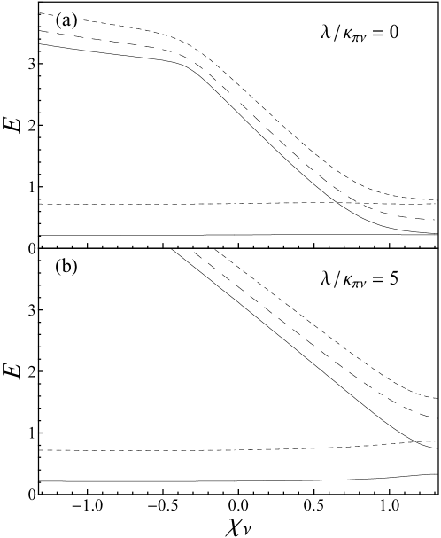
Figure 18: Excitation energies of the lowest $2^{+}$ (solid), $3^{+}$ (dashed), and $4^{+}$ (dotted) levels along the $\mathrm{SU}_{\pi\nu}(3)$–$\mathrm{SU}_{\pi\nu}^{*}(3)$ transition, (a) with no Majorana operator and (b) for $\lambda/\kappa_{\pi\nu}=5$. The change in slope for the excited band level energies at ${\chi_{\nu}}\approx-0.4$ in part (a) arises from the crossing of the scissors and $\gamma$ bands. Calculations are for ${\chi_{\pi}}=-\sqrt{7}/2$ and $N_{\pi}=N_{\nu}=5$, with minimal perturbations $\xi^{\prime}=0.95$ and for part (a) $\lambda/\kappa_{\pi\nu}=0.125$ to remove numerical degeneracies.

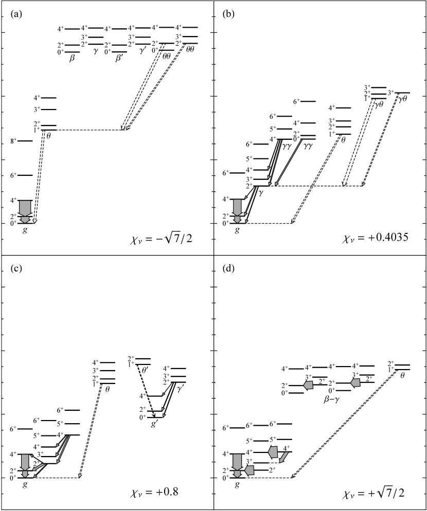
Figure 19: Level schemes for the $\mathrm{SU}_{\pi\nu}(3)$–$\mathrm{SU}_{\pi\nu}^{*}(3)$ transition with no Majorana operator: (a) the $\mathrm{SU}_{\pi\nu}(3)$ limit at ${\chi_{\nu}}=-\sqrt{7}/2$, (b) the second order transition point at ${\chi_{\nu}}\approx 0.4035$, (c) the approximate ground state crossing point at ${\chi_{\nu}}=0.8$, and (d) the $\mathrm{SU}_{\pi\nu}^{*}(3)$ limit at ${\chi_{\nu}}=+\sqrt{7}/2$. The $E2$ branching patterns are shown for selected band head states, and the ground state band $4^{+}\rightarrow 2^{+}$ and $2^{+}\rightarrow 0^{+}$ transitions are included for scale [shaded arrows, widths proportional to $B(E2)$ strength]. The $M1$ transitions deexciting the scissors band head states are shown as well [dashed arrows, widths proportional to $B(M1)$ strength]. The $g$ (ground), $\beta$, $\gamma$, and $\theta$ (scissors) band designations are schematic (see text). All panels share a common energy scale. Calculations are for ${\chi_{\pi}}=-\sqrt{7}/2$ and $N_{\pi}=N_{\nu}=5$, with minimal perturbations $\xi^{\prime}=0.95$ for part (a) and $\lambda/\kappa_{\pi\nu}=0.125$ for part (d) to remove numerical degeneracies.

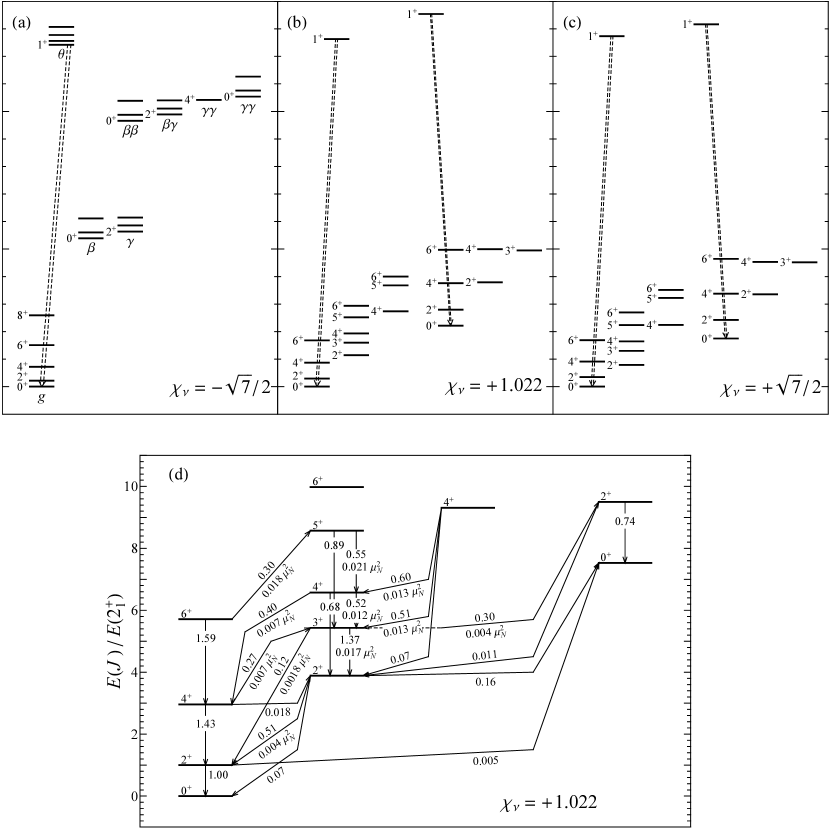
Figure 20: Level schemes for the $\mathrm{SU}_{\pi\nu}(3)$–$\mathrm{SU}_{\pi\nu}^{*}(3)$ transition with Majorana contribution $\lambda/\kappa_{\pi\nu}=5$: (a) the $\mathrm{SU}_{\pi\nu}(3)$ limit at ${\chi_{\nu}}=-\sqrt{7}/2$, (b) the second order transition point at ${\chi_{\nu}}\approx 1.022$, and (c) the $\mathrm{SU}_{\pi\nu}^{*}(3)$ limit at ${\chi_{\nu}}=+\sqrt{7}/2$. For the transition point, $B(E2)$ and $B(M1)$ strengths among selected low-lying levels are given if part (d). Parts (a)–(c) share a common energy scale, while energies in part (d) are normalized to the $2^{+}_{1}$ level energy. Dashed arrows in parts (a)–(c) indicate $M1$ transitions from the scissors excitations. $B(E2)$ and $B(M1)$ strengths in part (d) are shown spin-descending, with $B(E2)$ strengths normalized to $B(E2;2^{+}_{1}\rightarrow 0^{+}_{1})$ [$0.283\,e^{2}\mathrm{b}^{2}$]. The $g$ (ground), $\beta$, $\gamma$, and $\theta$ (scissors) band designations are schematic. Calculations are for ${\chi_{\pi}}=-\sqrt{7}/2$ and $N_{\pi}=N_{\nu}=5$, with a minimal $\hat{n}_{d}$ perturbation $\xi^{\prime}=0.95$ for part (a) to remove numerical degeneracies.

In the $\mathrm{SU}_{\pi\nu}(3)$ limit [Fig. 19(a)], the lowest excitation above the ground state band ($F=F_{\text{max}}$) is the scissors mode ($F=F_{\text{max}}-1$), followed at higher energy by a cluster of degenerate $K=0$ and $2$ excitations. These arise from proton-neutron symmetric beta and gamma oscillations ($F=F_{\text{max}}$), asymmetric beta and gamma oscillations ($F=F_{\text{max}}-1$), and two-phonon scissors oscillations ($F=F_{\text{max}}-2$). All $E2$ transitions from the excited bands to the ground state band vanish exactly for the $\mathrm{SU}_{\pi\nu}(3)$ dynamical symmetry, but for small breakings of the symmetry they approximately follow the rotational Alaga rules. $M1$ transitions vanish as well, except those involving excitations of the scissors mode.

The level scheme for the $\mathrm{SU}_{\pi\nu}(3)$–$\mathrm{SU}_{\pi\nu}^{*}(3)$ second order transition point (${\chi_{\nu}}\approx 0.4035$) is shown in Fig. 19(b). As ${\chi_{\nu}}$ is increased from $-\sqrt{7}/2$, one of the $\gamma$ bands (no longer of pure $F$ spin) rapidly descends to lower excitation energy. At the transition point, this band is connected to the ground state band by $E2$ transitions $\sim 1/10$ as strong as in-band transitions. The $M1$ admixtures are extremely large, with $B(M1)/B(E2)\sim 1\mu_{N}^{2}/(e^{2}\mathrm{b}^{2})$, both for the $\gamma$ to ground and the in-band transitions. The $\gamma$ band is followed in its descent by a series of $K=4$, $6$, $\ldots$ bands, originating as two-phonon, three-phonon, etc., $\gamma$ excitations. However, the $K=0$ two-phonon $\gamma$ excitation does not descend as rapidly and thus has a positive anharmonicity, $\sim 2.8$ at the transition point. Positive anharmonicity of this band has also recently been discussed as a signature of the axial-triaxial transition both in the one-fluid IBM [62] and in the $\mathrm{Y}(5)$ geometric model [63]. [The irregular level spacing seen in this band in Fig. 19(b) is not a fundamental signature but rather arises from mixing with the nearly degenerate scissors band for these parameter values.] As the $\gamma$ vibrational energy scale decreases, the $K=1$ and $3$ $\gamma$ exitations of the scissors band similarly approach the scissors band in energy.

Although the coherent state energy surface first becomes soft to triaxial deformations at the second order transition point, it is only for ${\chi_{\nu}}\gtrsim 0.65$ that highly triaxial configurations like that of Fig. 1 become lower in energy than axial configurations. A level scheme obtained in this regime, at ${\chi_{\nu}}=0.8$, is shown in Fig. 19(c). The ground state band and first $K=2$ and $4$ bands are close in energy, resembling the $\mathrm{SU}_{\pi\nu}^{*}(3)$ ground state representation. The relative $E2$ transition strengths are intermediate between those for the $\mathrm{SU}_{\pi\nu}(3)$ and $\mathrm{SU}_{\pi\nu}^{*}(3)$ symmetries. The first excited $K=0$ band and following $K=2$ band, in contrast, have relative energies more appropriate to a ground state and its associated $\gamma$ excitation, and $B(E2)$ values closely matching the $\mathrm{SU}_{\pi\nu}(3)$ Alaga rules. The energy spacing scales within these bands is less (by $\sim 10\%$) than that of the ground state family of bands, suggesting a different moment of inertia or different triaxial nature to the rotation. The excitation energy of the $0^{+}_{2}$ state reaches its lowest value along the $\mathrm{SU}_{\pi\nu}(3)$–$\mathrm{SU}_{\pi\nu}^{*}(3)$ transition at approximately this ${\chi_{\nu}}$ value. The observables are thus highly suggestive of an avoided crossing between an $\mathrm{SU}_{\pi\nu}^{*}(3)$-like configuration and an $\mathrm{SU}_{\pi\nu}(3)$-like configuration, although the actual eigenstate structure is presumably more complicated. An apparent avoided crossing also occurs between $1^{+}$ scissors excitations based upon these configurations.

We now briefly reconsider the $\mathrm{SU}_{\pi\nu}(3)$–$\mathrm{SU}_{\pi\nu}^{*}(3)$ transition for a realistic Majorana operator strength ($\lambda/\kappa_{\pi\nu}=5$) [Figs. 18(b) and 20]. At the $\mathrm{SU}_{\pi\nu}(3)$ limit, the eigenstates are unchanged, but the levels with $F<F_{\text{max}}$ are raised in energy [Fig. 20(a)]. The lowest-lying excitations are thus proton-neutron symmetric $\beta$ and $\gamma$ excitations, followed at higher energies by the symmetric $\beta$ and $\gamma$ multiphonon excitations. The second-order transition between axial and triaxial equilibrium occurs at much larger ${\chi_{\nu}}$ than without the Majorana operator, ${\chi_{\nu}}\approx 1.022$ (Fig. 14). The level scheme for the transition point [Fig. 20(b)] shows large differences between ground state and excited families of levels. The lowest $K=0$, $2$, and $4$ quasi-bands have level spacings intermediate between those for the $\mathrm{SU}_{\pi\nu}(3)$ and $\mathrm{SO}_{\pi\nu}(6)$ symmetries. The next $K=0$ quasi-band is far less rotational in spacing and has a $2^{+}$-$0^{+}$ energy spacing about twice as large as for the ground state. The levels above it are assembled into an approximate $\mathrm{SO}_{\pi\nu}(6)$ multiplet structure. All $M1$ strengths are attenuated relative to the cases with no Majorana contribution, with a typical admixture scale $B(M1)/B(E2)\sim 0.05\mu_{N}^{2}/(e^{2}\mathrm{b}^{2})$. Qualitatively, little further changes as ${\chi_{\nu}}$ increases to $+\sqrt{7}/2$ [Fig. 20(c)], except that the ground state family of levels takes on more distinctly $\mathrm{SO}_{\pi\nu}(6)$-like energy spacings and $B(E2)$ strengths.

5.3 The $\mathrm{U}_{\pi\nu}(5)$–$\mathrm{SU}_{\pi\nu}^{*}(3)$ transition

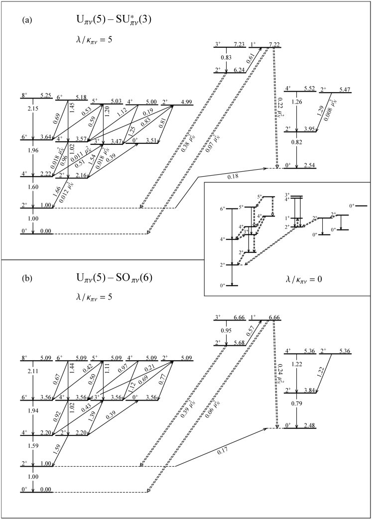
Figure 21: Level schemes for the second order transition points along (a) the $\mathrm{U}_{\pi\nu}(5)$–$\mathrm{SU}_{\pi\nu}^{*}(3)$ transition and (b) the $\mathrm{U}_{\pi\nu}(5)$–$\mathrm{SO}_{\pi\nu}(6)$ transition, calculated for a Majorana operator strength of $\lambda/\kappa_{\pi\nu}=5$. The inset to part (a) shows the corresponding level scheme with no Majorana operator. Energies are indicated normalized to the $2^{+}_{1}$ level energy. $B(E2)$ strengths are shown spin-descending, normalized to $B(E2;2^{+}_{1}\rightarrow 0^{+}_{1})$ separately in each panel [$0.175\,e^{2}\mathrm{b}^{2}$ for part (a), $0.168\,e^{2}\mathrm{b}^{2}$ for part (b)], and selected $B(M1)$ strengths are indicated as well. Dashed double arrows indicate selected strong $M1$ transitions. Calculations are for $N_{\pi}=N_{\nu}=5$, with ${\chi_{\pi}}=-\sqrt{7}/2$, ${\chi_{\nu}}=+\sqrt{7}/2$, and $\xi^{\prime}=0.2$ for part (a) and with ${\chi_{\pi}}=0$, ${\chi_{\nu}}=0$, and $\xi^{\prime}=0.2$ for part (b).

The basic spectroscopic features along the $\mathrm{U}_{\pi\nu}(5)$–$\mathrm{SU}_{\pi\nu}^{*}(3)$ transition differ fundamentally depending upon whether or not a realistic Majorana contribution is included in the Hamiltonian. The level scheme for the $\mathrm{U}_{\pi\nu}(5)$ symmetry of the IBM-2 [3, 9] exhibits extreme degeneracies if no Majorana operator is present: there are two degenerate one-phonon $2^{+}$ levels (one fully symmetric and one of mixed symmetry) and eleven degenerate levels of various symmetry in the two-phonon multiplet. By the second order transition point ($\xi^{\prime}=1/5$), these highly degenerate levels evolve into a cluster of low-lying excitations of widely varying $F$-spin content, shown in the inset to Fig. 21(a). Among these levels, incipient forms of the $\mathrm{SU}_{\pi\nu}^{*}(3)$ ground-state and scissors quasi-band structures are apparent. The electromagnetic transition properties are dominated by the ubiquity of strong $M1$ transitions, arising from the mixing of $\mathrm{U}_{\pi\nu}(5)$ states of different $F$ spin. For instance, both the $2^{+}_{2}\rightarrow 2^{+}_{1}$ and $2^{+}_{3}\rightarrow 2^{+}_{1}$ transitions have $B(M1)$ strengths $>0.1\,\mu_{N}^{2}$, typical of mixed symmetry state decays.

If instead a realistic Majorana operator strength $\lambda/\kappa_{\pi\nu}\approx 5$ is considered, the low-energy excitation spectrum simplifies considerably, as shown in Fig. 21(a). The low-lying levels have nearly pure $F\approx F_{\text{max}}$, with a few per cent admixtures of other $F$ values, and are grouped into approximate $SO(5)$ multiplets. Mixed symmetry levels of $F\approx F_{\text{max}}-1$ are present at higher energy ($1^{+}$, $2^{+}$, and $3^{+}$ levels at top of figure). The $T$ parity is a good quantum number throughout the $\mathrm{U}_{\pi\nu}(5)$–$\mathrm{SU}_{\pi\nu}^{*}(3)$ transition, so $T$ parity selection rules apply to the electromagnetic transitions. The level scheme and $E2$ transition strengths are nearly identical to those obtained for the second order transition point between $\mathrm{U}_{\pi\nu}(5)$ and $\mathrm{SO}_{\pi\nu}(6)$, shown for comparison in Fig. 21(b). There is thus also considerable resemblance to the predictions of the geometric $E(5)$ model [64, 65]. Two features of the $\mathrm{U}_{\pi\nu}(5)$–$\mathrm{SU}_{\pi\nu}^{*}(3)$ transition point spectrum allow it to be distinguished from the $\mathrm{U}_{\pi\nu}(5)$–$\mathrm{SO}_{\pi\nu}(6)$ case. First, a slight breaking of the degeneracy of the $SO(5)$ multiplets occurs, in the sense necessary to create the $\mathrm{SU}_{\pi\nu}^{*}(3)$ quasi-bands. Thus, the $2^{+}_{2}$ level moves below the $4^{+}_{1}$ level, the $3^{+}_{1}$ and $4^{+}_{2}$ levels move below the $6^{+}_{1}$ level, etc. This effect becomes much more marked just past the transition point. Second, sizeable $M1$ transition strengths, $B(M1)/B(E2)\approx 0.05\,\mu_{N}^{2}/(e^{2}\mathrm{b}^{2})$ to $0.1\,\mu_{N}^{2}/(e^{2}\mathrm{b}^{2})$, are present among the low-lying levels [Fig. 21(a)], while these vanish when ${\chi_{S}}=0$. Such $M1$ admixtures in general play an essential role in identifying deviations from ${\chi_{V}}=0$ [66, 67, 57].

6 Conclusion

The IBM-2 phase diagram investigated here provides a framework for studying the transition between axial and triaxial structure in nuclei. Triaxial deformation might arise from several possible sources: distinct deformations of the proton and neutron fluids as considered in the present work, higher-order interactions in an essentially one-fluid nucleus [28], or the presence of configurations involving hexadecapole nucleon pairs [68]. The main spectroscopic features of proton-neutron triaxial structure are exemplified by the $\mathrm{SU}_{\pi\nu}^{*}(3)$ dynamical symmetry, shown in Fig. 17(a). Proton-neutron triaxiality is characterized by a low-lying $K=2$ band, as in the other forms of nuclear triaxiality, but with level energies following a rotational $L(L+1)$ sequence. The $B(E2)$ strength pattern is remarkably similar to that of the classic rigid triaxial rotor of the Davydov model, including the unusual feature that $B(E2;2^{+}_{2}\rightarrow 0^{+}_{1})=0$ (this however only strictly holds for $N_{\pi}=N_{\nu}$ and $e_{\pi}=e_{\nu}$). The microscopic conditions leading to two-fluid triaxial structure, which requires ${\chi_{\pi}}$ and ${\chi_{\nu}}$ of opposite sign, are found when the proton bosons are particle like (below mid-shell) and the neutron bosons are hole-like (above mid-shell) or vice versa. Nuclei in this category include the heavy $\mathrm{Ru}$ and $\mathrm{Pd}$ isotopes [69, 67, 70], the light rare earth nuclei below the $N=82$ shell closure, and the extremely light $\mathrm{W}$, $\mathrm{Os}$, and $\mathrm{Pt}$ nuclei.

The $\mathrm{SU}_{\pi\nu}^{*}(3)$ dynamical symmetry probably does not occur in its pure form in any actual nuclei. In this article, we have seen how the features of $\mathrm{SU}_{\pi\nu}^{*}(3)$ proton-neutron triaxiality are modified by the Majorana interaction [Fig. 17(b,c)], which tends to alter the spectrum towards that for the $\mathrm{SO}_{\pi\nu}(6)$ dynamical symmetry. Of most importance from a phenomenological viewpoint, we have investigated the transition from axially symmetric deformed [$\mathrm{SU}_{\pi\nu}(3)$-like] to triaxially deformed [$\mathrm{SU}_{\pi\nu}^{*}(3)$-like] structure, either without [Fig. 19] or with [Fig. 20] a Majorana interaction. In particular, Fig. 20 represents a realistic study of this transition, including the behavior of the lowest $K=1$, or scissors, band. It is found that, despite the attenuation of proton-neutron triaxial features by the Majorana interaction, two-fluid triaxiality can serve as the underlying mechanism driving one-fluid triaxiality, and recognizable features of its two-fluid nature can remain even in the presence of realistic Majorana interactions. The two-fluid phenomena are likely to take on more importance as very neutron rich nuclei become accessible to experimental study. When the valence protons and neutrons occupy well-separated orbitals, the proton-neutron interaction strengths are reduced, yielding a situation seen in Sec. 4 to be much more conducive to true two-fluid triaxiality.

The present analysis may also serve as a model for the study of other multi-fluid bosonic systems. Within nuclear physics, the $\mathrm{U}_{\text{core}}(6)\otimes\mathrm{U}_{\text{skin}}(6)$ description of core-skin collective modes in neutron rich nuclei [71] is most directly analogous. In molecular physics, the $U_{1}(4)\otimes U_{2}(4)$ vibron model with two vibronic species [4] may be studied similarly. The appropriate coherent state formalism is discussed in Ref. [72]. The phase transition in this model is relevant to coupled vibronic bending modes in “floppy” molecules such as acetylene [73]. An extreme case of a multi-fluid algebraic model is found in applications to polymers, in which an arbitarily large number of vibronic fluids are coupled [74]. Yet another case is that of atomic condensates, for which scissors modes of a single-constituent Bose-Einstein condensate relative to an anisotropic potential have been observed [75]. Experiments have been planned to produce condensates of two atomic species. The exotic features of the IBM-2 phase diagram are likely to be encountered for other multi-fluid systems as well. They highlight the need for a classification scheme beyond the simple Ehrenfest or one-parameter Landau models to address the phase structure of systems which simultaneously possess multiple control parameters and multiple order parameters.

Appendix A Matrix element of an arbitrary $m$-body operator between multi-fluid coherent states

For calculations in the coherent state formalism involving multi-fluid operators, it is useful to deduce a general formula for the matrix element of an arbitrary $m$-body operator between arbitrary multi-fluid coherent states. Define $S$ different coherent boson species $B_{s}^{\dagger}$ ($s=1,\ldots,S$) in terms of the basic boson operators $b_{i}^{\dagger}$ ($i=1,\ldots,n$) as orthonormal linear combinations

$$B_{s}^{\dagger}\equiv\sum_{i=1}^{n}\alpha_{s,i}b_{i}^{\dagger},$$ (A.1)

where $\sum_{i=1}^{n}\alpha_{s^{\prime},i}^{*}\alpha_{s,i}=\delta_{s^{\prime},s}$. Then the multi-species coherent states

$$\lvert N_{1}\cdots N_{S}\rangle\equiv\Bigl{(}\prod_{s=1}^{S}\frac{1}{\sqrt{N_{s}!}}(B_{s}^{\dagger})^{N_{s}}\Bigr{)}|0\rangle$$ (A.2)

are normalized, are orthogonal to each other for different $N_{s}$ values, and have good total boson number $N=\sum_{s=1}^{S}N_{s}$, where the total boson number operator is $\hat{N}\equiv\sum_{i=1}^{n}b_{i}^{\dagger}b_{i}$. Coherent states of the type (A.2) also arise in the study of intrinsic excitations in algebraic models. In this context, the different coherent boson operators $B_{s}^{\dagger}$ represent a ground state condensate and one or more orthogonal excitation modes (see, e.g., Refs. [76, 77, 78, 72, 79]).

The matrix element of an arbitrary $m$-body operator ($m\geq 1$) between two arbitrary multi-species coherent states is [80]

$$\langle N_{1}^{\prime}\cdots N_{S}^{\prime}\rvert\Bigl{(}\prod_{i=1}^{m}b_{r_{i}^{\prime}}^{\dagger}\Bigr{)}\Bigl{(}\prod_{i=1}^{m}b_{r_{i}}\Bigr{)}|N_{1}\cdots N_{S}\rangle\\ =\sum_{\begin{subarray}{c}t_{1}^{\prime},\ldots,t_{m}^{\prime}\\ t_{1},\ldots,t_{m}\end{subarray}=1}^{S}\Bigl{[}\prod_{s=1}^{S}\delta_{N_{s}^{\prime}-\nu_{s}^{\prime},N_{s}-\nu_{s}}\sqrt{N_{s}^{\prime\underline{\nu_{s}^{\prime}}}N_{s}^{\underline{\nu_{s}}}}\Bigr{]}\Bigl{(}\prod_{i=1}^{m}\alpha_{t_{i}^{\prime},r_{i}^{\prime}}^{*}\alpha_{t_{i},r_{i}}\Bigr{)},$$ (A.3)

where $\nu_{s}\equiv\sum_{i=1}^{m}\delta_{t_{i},s}$, $\nu_{s}^{\prime}\equiv\sum_{i=1}^{m}\delta_{t_{i}^{\prime},s}$, and an underlined superscript indicates the falling factorial [$m^{\underline{n}}\equiv m(m-1)\cdots(m-n+1)$] [81]. The multiple sum in (A.3) nominally contains $S^{2m}$ terms, but only those with $N_{s}^{\prime}-\nu_{s}^{\prime}=N_{s}-\nu_{s}$ and $N_{s}-\nu_{s}\geq 0$ can yield nonzero contributions. Three stages are involved in evaluating the matrix element of a general operator: reexpression of the operator in terms of normal-ordered $m$-body terms, evaluation of the matrix elements of these by (A.3), and simplification of the result. These steps can all readily be carried out though computer-based symbolic manipulation.

Appendix B Properties of $F(a;x)$

The IBM-2 energy surface considered in Secs. 3 and 4 involves terms of the form

$$F(a;x)\equiv\frac{x(1+ax)}{1+x^{2}}.$$ (B.1)

We summarize here the extremum properties of this expression. For any value of the parameter $a$, $F(a;x)$ has two extrema with respect to $x$, at

$$x_{\pm}(a)\equiv a\pm\sqrt{a^{2}+1},$$ (B.2)

The global minimum of $F(a;x)$ is located at $x_{-}(a)$, and the global maximum is located at $x_{+}(a)$. Note that $x_{-}(a)<0$, $x_{+}(a)>0$, and the two extremum positions are related by $x_{-}(a)x_{+}(a)=-1$. The extremal values of $F$ are simply

$$F[a;x_{\pm}(a)]=\frac{1}{2}x_{\pm}(a).$$ (B.3)

If $a>0$ then $\lvert F[a;x_{-}(a)]\rvert<\lvert F[a;x_{+}(a)]\rvert$, while for $a<0$ the inequality holds in the opposite sense.

References

- [1] R. Gilmore, J. Math. Phys. 20 (1979) 891.
- [2] D. H. Feng, R. Gilmore, and S. R. Deans, Phys. Rev. C 23 (1981) 1254.
- [3] F. Iachello and A. Arima, The Interacting Boson Model (Cambridge University Press, Cambridge, 1987).
- [4] F. Iachello and R. D. Levine, Algebraic Theory of Molecules (Oxford University Press, Oxford, 1995).
- [5] A. E. L. Dieperink, O. Scholten, and F. Iachello, Phys. Rev. Lett. 44 (1980) 1747.
- [6] A. Arima, T. Otsuka, F. Iachello, and I. Talmi, Phys. Lett. B 66 (1977) 205.
- [7] T. Otsuka, A. Arima, F. Iachello, and I. Talmi, Phys. Lett. B 76 (1978) 139.
- [8] T. Otsuka, A. Arima, and F. Iachello, Nucl. Phys. A 309 (1978) 1.
- [9] P. Van Isacker, K. Heyde, J. Jolie, and A. Sevrin, Ann. Phys. (N.Y.) 171 (1986) 253.
- [10] A. E. L. Dieperink and R. Bijker, Phys. Lett. B 116 (1982) 77.
- [11] M. A. Caprio, in Ref. [82], p. 215.
- [12] M. A. Caprio and F. Iachello, Phys. Rev. Lett. 93 (2004) 242502.
- [13] J. M. Arias, J. Dukelsky, and J. E. García-Ramos, in Ref. [82], p. 127.
- [14] J. M. Arias, J. Dukelsky, and J. E. García-Ramos, Phys. Rev. Lett. 93 (2004) 212501.
- [15] A. de-Shalit and I. Talmi, Nuclear Shell Theory, No. 14 in Pure and Applied Physics (Academic, New York, 1963).
- [16] A. E. L. Dieperink and I. Talmi, Phys. Lett. B 131 (1983) 1.
- [17] N. R. Walet and P. J. Brussaard, Nucl. Phys. A 474 (1987) 61.
- [18] A. Sevrin, K. Heyde, and J. Jolie, Phys. Rev. C 36 (1987) 2621.
- [19] A. Sevrin, K. Heyde, and J. Jolie, Phys. Rev. C 36 (1987) 2631.
- [20] A. Leviatan and M. W. Kirson, Ann. Phys. (N.Y.) 201 (1990) 13.
- [21] J. N. Ginocchio and A. Leviatan, Ann. Phys. (N.Y.) 216 (1992) 152.
- [22] M. A. Caprio, in Nuclei and Mesoscopic Physics, edited by V. Zelevinsky et al. (AIP, Melville, NY, in press).
- [23] R. Gilmore, C. M. Bowden, and L. M. Narducci, Phys. Rev. A 12 (1975) 1019.
- [24] W. Zhang, D. H. Feng, and R. Gilmore, Rev. Mod. Phys. 62 (1990) 867.
- [25] J. N. Ginocchio and M. W. Kirson, Phys. Rev. Lett. 44 (1980) 1744.
- [26] J. N. Ginocchio and M. W. Kirson, Nucl. Phys. A 350 (1980) 31.
- [27] A. E. L. Dieperink and O. Scholten, Nucl. Phys. A 346 (1980) 125.
- [28] P. Van Isacker and Jin-Quan. Chen, Phys. Rev. C 24 (1981) 684.
- [29] A. Leviatan, Ann. Phys. (N.Y.) 179 (1987) 201.
- [30] E. López-Moreno and O. Castaños, Phys. Rev. C 54 (1996) 2374.
- [31] P. Ehrenfest, Proc. Amsterdam. Acad. 36 (1933) 153.
- [32] A. E. L. Dieperink, Nucl. Phys. A 421 (1984) 189c.
- [33] R. Bijker, Phys. Rev. C 32 (1985) 1442.
- [34] A. Van Egmond and K. Allaart, Phys. Lett. B 164 (1985) 1.
- [35] A. Bohr and B. R. Mottelson, Nuclear Deformations, Vol. 2 of Nuclear Structure (World Scientific, Singapore, 1998).
- [36] M. E. Rose, Elementary Theory of Angular Momentum (Wiley, New York, 1957).
- [37] A. B. Balanktekin, B. R. Barrett, and S. Levit, Phys. Lett. B 129 (1983) 153.
- [38] P. O. Lipas, P. von Brentano, and A. Gelberg, Rep. Prog. Phys. 53 (1990) 1355.
- [39] L. D. Landau and E. M. Lifschitz, Statistical Physics, Part 1, Vol. 5 of Course of Theoretical Physics (Butterworth Heinemann, Oxford, 1980), translated by J. B. Sykes and M. J. Kearsley.
- [40] J. Jolie, R. F. Casten, P. von Brentano, and V. Werner, Phys. Rev. Lett. 87 (2001) 162501.
- [41] R. Gilmore, Catastrophe Theory for Scientists and Engineers (Wiley, New York, 1981).
- [42] I. Talmi, Simple Models of Complex Nuclei: The Shell Model and Interacting Boson Model, Vol. 7 of Contemporary Concepts in Physics (Harwood Academic Publishers, Chur, Switzerland, 1993).
- [43] A. Novoselsky and I. Talmi, Phys. Lett. B 172 (1986) 139.
- [44] J. Dobaczewski, W. Nazarewicz, J. Skalski, and T. Werner, Phys. Rev. Lett. 60 (1988) 2254.
- [45] O. Scholten, Phys. Lett. B 119 (1982) 5.
- [46] O. Scholten, Phys. Rev. C 28 (1983) 1783.
- [47] A. Van Egmond and K. Allaart, Nucl. Phys. A 425 (1984) 275.
- [48] O. Scholten, K. Heyde, P. Van Isacker, J. Jolie, J. Moreau, M. Waroquier, and J. Sau, Nucl. Phys. A 438 (1985) 41.
- [49] U. Hartmann, D. Bohle, T. Guhr, K. Hummel, G. Kilgus, U. Milkau, and A. Richter, Nucl. Phys. A 465 (1987) 25.
- [50] A. S. Davydov and G. F. Filippov, Nucl. Phys. 8 (1958) 237.
- [51] K. Heyde, P. Van Isacker, M. Waroquier, and J. Moreau, Phys. Rev. C 29 (1984) 1420.
- [52] R. F. Casten, P. von Brentano, K. Heyde, P. Van Isacker, and J. Jolie, Nucl. Phys. A 439 (1985) 289.
- [53] Y. F. Smirnov, N. A. Smirnova, and P. Van Isacker, Phys. Rev. C 61 (2000) 041302(R).
- [54] D. D. Warner and R. F. Casten, Phys. Rev. C 28 (1983) 1798.
- [55] T. Otsuka and N. Yoshida, User’s manual of the program NPBOS, JAERI-M 85-094 (1985).
- [56] J. P. Elliott, Proc. R. Soc. London A 245 (1958) 128.
- [57] T. Otsuka, Hyperfine Interact. 75 (1992) 23.
- [58] D. R. Bès, Nucl. Phys. 10 (1959) 373.
- [59] J. M. Eisenberg and W. Greiner, Nuclear Models: Collective and Single-Particle Phenomena, 3rd ed., Vol. 1 of Nuclear Theory (North-Holland, Amsterdam, 1987).
- [60] Y. Leschber and J. P. Draayer, Phys. Lett. B 190 (1987) 1.
- [61] H. Harter, A. Gelberg, and P. von Brentano, Phys. Lett. B 157 (1985) 1.
- [62] J. E. García-Ramos, C. E. Alonso, J. M. Arias, P. Van Isacker, and A. Vitturi, Nucl. Phys. A 637 (1998) 529.
- [63] F. Iachello, Phys. Rev. Lett. 91 (2003) 132502.
- [64] F. Iachello, Phys. Rev. Lett. 85 (2000) 3580.
- [65] R. F. Casten and N. V. Zamfir, Phys. Rev. Lett. 85 (2000) 3584.
- [66] P. Van Isacker, P. O. Lipas, K. Helimäki, I. Koivistoinen, and D. D. Warner, Nucl. Phys. A 476 (1988) 301.
- [67] Ka-Hae Kim, A. Gelberg, T. Mizusaki, T. Otsuka, and P. von Brentano, Nucl. Phys. A 604 (1996) 163.
- [68] K. Heyde, P. Van Isacker, M. Waroquier, G. Wenes, Y. Gigase, and J. Stachel, Nucl. Phys. A 398 (1983) 235.
- [69] P. Van Isacker and G. Puddu, Nucl. Phys. A 348 (1980) 125.
- [70] J. L. M. Duarte, T. Borello-Lewin, G. Maino, and L. Zuffi, Phys. Rev. C 57 (1998) 1539.
- [71] D. D. Warner and P. Van Isacker, Phys. Lett. B 395 (1997) 145.
- [72] A. Leviatan and M. W. Kirson, Ann. Phys. (N.Y.) 188 (1988) 142.
- [73] F. Pérez-Bernal et al. (in preparation).
- [74] F. Iachello and P. Truini, Ann. Phys. (N.Y.) 276 (1999) 120.
- [75] O. M. Maragò, S. A. Hopkins, J. Arlt, E. Hodby, G. Hechenblaikner, and C. J. Foot, Phys. Rev. Lett. 84 (2000) 2056.
- [76] A. Bohr and B. R. Mottelson, Physica Scripta 25 (1982) 28.
- [77] R. Bijker and A. E. L. Dieperink, Phys. Rev. C 26 (1982) 2688.
- [78] A. Leviatan, Z. Phys. A 321 (1985) 467.
- [79] A. Leviatan, Prog. Part. Nucl. Phys. 24 (1990) 85.
- [80] M. A. Caprio, J. Phys. A (in press).
- [81] R. L. Graham, D. E. Knuth, and O. Patashnik, Concrete Mathematics: A Foundation for Computer Science, 2nd ed. (Addison-Wesley, Reading, MA, 1994).
- [82] R. Bijker, R. F. Casten, and A. Frank, eds., Nuclear Physics, Large and Small: International Conference on Microscopic Studies of Collective Phenomena, AIP Conf. Proc. No. 726 (AIP, Melville, NY, 2004).