Coulomb distortion of relativistic electrons in the
nuclear electrostatic field

Abstract

Continuum states of the Dirac equation are calculated numerically for the electrostatic field generated by the charge distribution of an atomic nucleus. The behavior of the wave functions of an incoming electron with a given asymptotic momentum in the nuclear region is discussed in detail and the results are compared to different approximations used in the data analysis for quasielastic electron scattering off medium and highly charged nuclei. It is found that most of the approximations provide an accurate description of the electron wave functions in the range of electron energies above 100 MeV typically used in experiments for quasielastic electron scattering off nuclei only near the center of the nucleus. It is therefore necessary that the properties of exact wave functions are investigated in detail in order to obtain reliable results in the data analysis of quasielastic $(e,e^{\prime}p)$ knockout reactions or inclusive quasielastic $(e,e^{\prime})$ scattering. Detailed arguments are given that the effective momentum approximation with a fitted potential parameter is a viable method for a simplified treatment of Coulomb corrections for certain kinematical regions used in experiments. Numerical calculations performed within the framework of the single particle shell model for nucleons lead to the conclusion that our results are incompatible with calculations performed about a decade ago, where exact electron wave functions were used in order to calculate Coulomb corrections in distorted wave Born approximation. A discussion of the exact solutions of the Dirac equation for free electrons in a Coulomb field generated by a point-like charge and some details relevant for the numerical calculations are given in the appendix. Keywords: Coulomb corrections; Eikonal approximation; Quasielastic electron scattering PACS: 11.80.Fv; 25.30.Fj; 25.70.Bc

1 Introduction

Quasielastic $(e,e^{\prime}p)$ knockout reactions provide a powerful possibility to obtain information on the electromagnetic properties of nucleons embedded in the nuclear medium, since the transparency of the nucleus with respect to the electromagnetic probe makes it possible to explore the entire nuclear volume. Inclusive $(e,e^{\prime})$ scattering, where only the scattered electron is observed, provides information on a number of interesting nuclear properties like, e.g., the nuclear Fermi momentum [1], high-momentum components in nuclear wave functions [2], modifications of nucleon form factors in the nuclear medium [3], the scaling properties of the quasielastic response allow to study the reaction mechanism [4], and extrapolation of the quasielastic response to infinite nucleon number $A=\infty$ provides us with a very valuable observable of infinite nuclear matter [5]. There is now considerable theoretical and experimental interest in extracting longitudinal and transverse structure functions as a function of energy loss for fixed three momentum transfer for a range of nuclei [6]. In August 2005, the Thomas Jefferson National Accelerator Facility (TJNAF) Proposal E01-016, entitled ‘Precision measurement of longitudinal and transverse response functions of quasi-elastic electron scattering in the momentum transfer range $0.55$ GeV $\leq$ $|\vec{q}|$ $\leq$ $1.0$ GeV’ was approved such that the experiments will be performed in the near future at the TJNAF using ⁴He, ¹²C, ⁵⁶Fe and ²⁰⁸Pb as target nuclei.

The plane wave Born approximation is no longer adequate for the calculation of scattering cross sections in the strong and long-range electrostatic field of highly charged nuclei, and it has become clear in recent years that the correct treatment of the Coulomb distortion of the electron wave function due to the electrostatic field of the nucleus is unavoidable if one aims at a consistent interpretation of experimental data. E.g., it is still unclear whether the Coulomb sum rule is violated in nuclei [7].

Distorted wave Born approximation (DWBA) calculations with exact Dirac wave functions have been performed by Kim et al. [8] in the Ohio group and Udias et al. [9, 10] for quasielastic scattering off heavy nuclei. However, these calculations are cumbersome and difficult to control by people who were not directly involved in the development of the respective programs. Early DWBA calculations for ¹²C and ⁴⁰Ca were presented in [11]

Various approximate treatments have been proposed in the past for the treatment of Coulomb distortions [12, 13, 14, 15, 16, 17, 18, 19], and there is an extensive literature on the so-called eikonal approximation [20, 21, 22, 23, 24, 25, 26]. At lowest order, an expansion of the electron wave function in $\alpha Z$, where $\alpha$ is the fine-structure constant and $Z$ the charge number of the nucleus, leads to the well known effective momentum approximation (EMA) [27], which plays an important role in experimental data analysis and which will be explained below.

The effect of the charged nucleus on the electron wave function is twofold: Firstly, the (initial and final state) electron momentum $\vec{k}_{i,f}$ is enhanced in the vicinity of the nucleus due to the attractive electrostatic potential, i.e., the wave length of the electron is becoming shorter near the nucleus. Secondly, the attractive potential of the nucleus leads to a focusing of the electron wave function in the nuclear region. Solutions for the Dirac equation for the scattering of electrons in the nuclear field can be obtained from a partial wave expansion, where the radial Dirac equation must be solved numerically for each partial wave. To avoid such a computational effort, an approximate treatment is often adopted, based on a high-energy expansion in inverse powers of the electron energy [12, 13, 15]. The resulting expression for the distorted electron wave function is then expanded in powers of $\alpha Z$ as (we use units with $\hbar=c=1$ throughout)

$$\psi_{\tau}=e^{\pm i\delta_{1/2}}\frac{k^{\prime}}{k}e^{i\vec{k}^{\prime}\vec{r}}[1+g^{(1)}(a,b,\vec{k}^{\prime},\vec{r})+g^{(2)}(a,b,\vec{k}^{\prime},\vec{r})+...]u_{\tau},$$ (1)

where the sign $\pm$ refers to the two scattering solutions with outgoing or incoming spherical waves, respectively, whereas the corresponding indices $i,f$ are neglected for the sake of notational simplicity, $u_{\tau}$ is the plane wave spinor for the electron with a given helicity $\tau$ and $\vec{k}$ is the asymptotic electron momentum. For the case of a uniform spherical charge distribution of radius $R$, the values of $\vec{k}^{\prime},a,b$ and $\delta_{1/2}$ are given by [16]

$$k^{\prime}=k+\frac{3\alpha Z}{2R},\quad\delta_{1/2}=\alpha Z\biggl{(}\frac{4}{3}-\log 2kR\biggr{)}+b,$$

$$a=-\frac{\alpha Z}{6k^{\prime}R^{3}},\quad b=-\frac{3\alpha Z}{4k^{\prime 2}R^{2}},$$ (2)

with $\vec{k}^{\prime}$ parallel to $\vec{k}$. These values enter the first-order term according to

$$g^{(1)}=ar^{2}+iar^{2}\vec{k}^{\prime}\vec{r}\pm ib[(\vec{k}^{\prime}\times\vec{r})^{2}+2i\vec{k}^{\prime}\vec{r}-\vec{s}(\vec{k}^{\prime}\times\vec{r})],$$ (3)

where the spin operator $\vec{s}$ describes spin-dependent effects which are comparably small for higher electron energies. The meaning of the parameter $a$ can be easily understood from a semiclassical observation. For a highly relativistic electron with mass $m$ falling along the $z$-axis (i.e. with zero impact parameter and $k\gg V\gg m$) towards the nuclear center, the momentum inside the spherical charge distribution is given by

$${\tilde{k}}(z)=k-V(z),\quad V(r)=-\frac{3\alpha Z}{2R}+\frac{\alpha Z}{2R}\biggl{(}\frac{r}{R}\biggr{)}^{2}$$ (4)

where $V(r)$ is the electrostatic potential inside the charged sphere. Modifying the electron plane wave phase $e^{i\vec{k}\vec{r}}=e^{ikz}$ to $e^{ik^{\prime}z(1+az^{2})}$, as it is induced at lowest order by the second term in $g^{(1)}$, leads to the $z-$dependent electron momentum ${\tilde{k}}(z)$

$$\frac{1}{i}\frac{d}{dz}e^{ik^{\prime}z(1+az^{2})}=k^{\prime}(1+3az^{2})e^{ik^{\prime}z(1+az^{2})}={\tilde{k}}(z)e^{ik^{\prime}z(1+az^{2})}$$ (5)

in agreement with eq. (4). The parameter $b$ describes mainly the deformation of the wave front and can also be derived from semiclassical observations.

The standard method (in the case of light nuclei) to handle Coulomb distortions for elastic scattering in data analysis is the effective momentum approximation (EMA), which corresponds to the lowest order description of the Coulomb distortion in $\alpha Z$. EMA accounts for the two effects of the Coulomb distortion mentioned above (momentum modification and focusing) in the following way. For a highly relativistic electron with zero impact parameter the so-called effective momenta $k_{i,f}^{\prime}$ of the electron are given by

$$k_{i}^{\prime}=k_{i}+\Delta k,\quad k_{f}^{\prime}=k_{f}+\Delta k,\quad k_{i,f}=|\vec{k}_{i,f}|,\quad k_{i,f}^{\prime}=|\vec{k}_{i,f}^{\prime}|,\quad\Delta k=-V_{0}/c,$$ (6)

where $V_{0}$ is the potential energy of the electron in the center of the nucleus in analogy with eq. (2). E.g., for ²⁰⁸Pb we have $V_{0}\sim-25\,\mbox{MeV}$, not a negligible quantity when compared to energies of some hundreds of MeV typically used in electron scattering experiments. Cross sections are then calculated by using plane electron waves corresponding to the effective momenta instead of the asymptotic values in the matrix elements, and additionally one accounts for the focusing factors of the incoming and outgoing electron wave $k^{\prime}_{i}/k_{i}$ and $k^{\prime}_{f}/k_{f}$, which both enter quadratically into the cross sections. The main problem of the method is the fact that both the focusing and the electron momentum are not constant inside the nuclear volume. In the case of nucleon knockout reactions, most of the hit nucleons are located near the surface of the nucleus, where the classical momentum of the electrons is not given by the central value.

A strategy to remedy this defect is to alter the definition of the effective momenta by not using the central potential value $V_{0}$, but a value $V(r_{f})$ obtained from some fitting procedure (see also [28] and references therein). An even more ambitious strategy would be the introduction of two effective momenta, one which accounts for the average modification of the electron momentum inside the nucleus, and one which would be utilized for the calculation of the average focusing of the electron wave in the nuclear volume.

For quasielastic $(e,e^{\prime})$ scattering a comparison of EMA calculations with numerical results from the ‘exact’ DWBA calculation [29, 30] seems to indicate a failure of the EMA [31]. Also the improved approximation including a first order correction from eq. (3) is of limited validity. However, we find that the EMA with an effective potential $\bar{V}\sim(0.75...0.8)V_{0}$ for heavier nuclei represents a viable method for the analysis of Coulomb distortion effects in inclusive quasielastic electron scattering, if the initial and final energy of the electrons and the momentum transfer are sufficiently large.

2 Exact numerical calculations

2.1 Properties of exact wave functions

The nuclei of ⁴⁰Ca and ²⁰⁸Pb were chosen for our calculations as typical examples for medium and highly charged nuclei. The Dirac equation was solved by using a partial wave expansion, which is discussed in detail in the appendix. The radial integration of the radial functions was performed by the method presented in [32]. However, we did not neglect the electron mass in our calculations, although mass effects are quite small in our case.

We present results for an incoming electron with spin in direction of the electron momentum scattered off the fixed electrostatic potential of the nucleus. Considering different spin or final state waves with incoming spherical wave would lead basically to the same conclusions.

The charge distribution of the ²⁰⁸Pb nucleus was modeled by a Woods-Saxon distribution

$$\rho(r)=\frac{\rho_{0}}{e^{(r-r_{1/2})/a}+1}$$ (7)

with $r_{1/2}=6.6$ fm and diffusivity $a=0.545$ fm, compatible with an rms charge radius of $5.5$ fm and a central Coulomb potential of $V_{0}=-25.7$ MeV, whereas for the ⁴⁰Ca nucleus a three-parameter Fermi form was used

$$\rho(r)=\rho_{0}\frac{1+\omega(r/r_{1/2})^{2}}{e^{(r-r_{1/2})/a}+1}$$ (8)

with $r_{1/2}=3.766$ fm, diffusivity $a=0.586$ fm and $\omega=-0.161$, compatible with an rms charge radius of $3.48$ fm and a central Coulomb potential of $V_{0}=-10.4$ MeV [33, 34].

Fig. 1 shows the focusing $(\bar{\psi}\gamma^{0}\psi)^{1/2}$ of an electron wave incident on a ²⁰⁸Pb nucleus with an energy of $100$ MeV. The wave is normalized such that the density $\bar{\psi}\gamma^{0}\psi$ approaches the value $1$ in the asymptotic region.

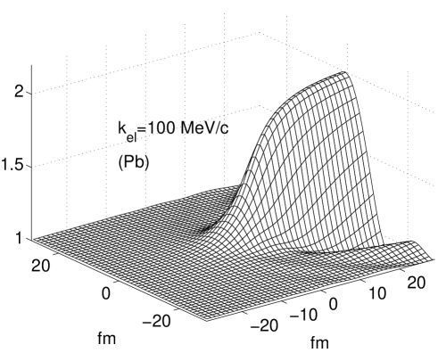
Figure 1: Amplitude $(\bar{\psi}\gamma^{0}\psi)^{1/2}$

of an electron wave incident on a ²⁰⁸Pb nucleus with an energy of $100$ MeV. The focusing varies strongly inside the nucleus, which has a radius of the order of $7$ fm.

The focusing is smaller in the upstream side of the nucleus and grows larger in the downstream side. At the same time, there is a strong decrease of the charge density in transverse direction to the electron momentum.

As a first step, we checked the focusing factor in the center ($r=0$) of the ²⁰⁸Pb nucleus. The exact central focusing factor and the value typically used in the EMA match extremely well already at relatively low energies above $40$ MeV, as shown in Fig. 2. For an electron energy of $100$ MeV the EMA focusing factor is given by $(100+25.7)/100=1.257$, as shown in Fig. (2), and the exact value deviates less than half a percent from this approximate result. This positive result turned out to be generally valid for ‘well-behaved’ types of potentials like, e.g., Gaussian potentials with depth and spatial extension comparable to depth and extension of the nuclear potential. But a closer look at the electron-wave amplitude reveals that the amplitude varies strongly inside the nuclear volume and the average focusing deviates from the value calculated from the electrostatic potential $V_{0}$ in the center of the nucleus.

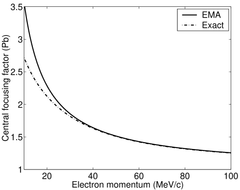
Figure 2: Focusing factor of the electron wave incident on a ²⁰⁸Pb nucleus as a function of the asymptotic electron momentum.

Fig. 3 shows the decay of the wave amplitude on an axis perpendicular to the electron momentum which goes through the nuclear center for an electron incident on ²⁰⁸Pb with an energy of $400$ MeV. The central focusing factor $\sim 425.7/400\sim 1.0642$ decreases to 1.0187 at the outer edge of the nucleus at a transverse distance of $8$ fm to the center.

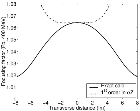
Figure 3: Focusing factor of the electron wave incident on ²⁰⁸Pb with electron energy $400$ MeV, on a straight line through the nuclear center transverse to the electron momentum.

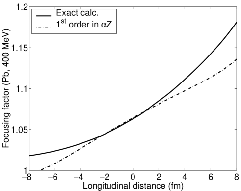
Figure 4: Focusing factor of the electron wave incident on ²⁰⁸Pb with electron energy $400$ MeV, along a straight line through the nuclear center parallel to the electron momentum.

Plotting the focusing factor along the axis through the nuclear center parallel to the electron momentum shows a strong increase on the downstream side of the nucleus (Fig. 4).

One is therefore naturally lead to the idea to calculate an averaged focusing factor $\bar{f}$ defined by

$$\bar{f}^{\,2}=\frac{\int d^{3}r\bar{\psi}_{\tau}(\vec{r})\gamma^{0}\psi_{\tau}(\vec{r})\rho(r)}{\int d^{3}r\rho(r)},$$ (9)

where $\rho(r)$ is the nuclear matter density distribution which can be well approximated by the charge density profile of the nucleus for sufficiently large mass numbers $A>20$. For a typical electron energy of $400$ MeV, one obtains $\bar{f}=1.050$ for ²⁰⁸Pb, corresponding to an effective potential value of $-20.07$ MeV, in contrast to the often used potential depth $V_{0}=-25.7$ MeV. The same calculation for ⁴⁰Ca leads to an effective potential of $-7.76$ MeV, compared to $V_{0}=-10.4$ MeV.

Defining an effective potential value $\bar{V}$ by

$$\bar{V}=\frac{\int d^{3}r\bar{\psi}_{\tau}(\vec{r})\gamma^{0}\psi_{\tau}(\vec{r})\rho(r)V(r)}{\int d^{3}r\bar{\psi}_{\tau}(\vec{r})\gamma^{0}\psi_{\tau}(\vec{r})\rho(r)},$$ (10)

which is a measure for the average (semiclassical) electron momentum inside the nuclear medium, leads to the very similar results $\bar{V}=20.12$ MeV for ²⁰⁸Pb and $\bar{V}=7.78$ MeV for ⁴⁰Ca. The difference between the effective momenta for the ingoing and outcoming electron calculated from this effective potential value can also be viewed as the effective momentum transferred by the electron to the nucleon in a quasielastic knockout process.

These observations are a strong argument that a modification of the EMA with an effective momentum corresponding to an effective potential $\sim(0.75...0.8)V_{0}$ would provide reasonable results when experimental data are corrected due to Coulomb distortion effects. An effective potential value of $(18.7\pm 1.5)$ MeV for ²⁰⁸Pb was extracted by Guèye et al. [35] by comparing data from quasielastic positron scattering to quasielastic electron scattering data taken by Zghiche et al. [36]. Exact calculations which include the Coulomb distortions of positrons will be presented in a forthcoming paper.

It is interesting to note that also for lighter nuclei like ⁴⁰Ca a similar effective potential value should be used like in the case of heavy nuclei. But in such cases, Coulomb distortions are usually of minor importance for the data analysis, and the choice of the effective potential value that is used in the EMA analysis plays a minor role.

We further mention that the average potential inside a homogeneously charged sphere is given by $4V_{0}/5$, where $V_{0}=-3\alpha Z/2R$ is the value of the potential in the center of the sphere. For positrons, we found that the same effective potential (with opposite sign) can be used, since the absolute values of the effective potentials differ by less than $0.05$ MeV for an energy range of several hundred MeV.

The first order term $g^{(1)}$ in eq. (1) fails to provide a satisfactory picture of the focusing inside the nucleus. It does not reproduce the strong increase of the focusing on the downstream side of nucleus, and the decrease of the focusing in transverse direction is also not contained. On the contrary, the dominant imaginary term $ib(\vec{k}^{\prime}\times\vec{r})^{2}$ causes an increase of the modulus of $1+g^{(1)}$ in transverse direction. The first order term $g^{(1)}$ accounts for the deformation of the wave front near the nuclear center, but higher order terms are needed in order to describe correctly the amplitude of the distorted electron wave inside the nucleus. Calculations with a phenomenological expression for the second order term $g^{(2)}$ have been presented in [16]. The dash-dotted lines in Figs. 3 and 4 show the focusing that would be obtained from the first order expression $(k^{\prime}/k)|1+g^{(1)}|$ for a homogeneously charged sphere with a radius $R=7.1$ fm and $Z=82$, which is a good approximation for a ²⁰⁸Pb nucleus.

It is solely the $a_{1}r^{2}$-term which accounts for a decrease of the focusing in transverse direction, but even if one neglects the other terms in $g^{(1)}$ which cause an increase of the focusing in transverse direction, the $a_{1}r^{2}$-term leads to a negligible effect compared to the actual transverse decrease of the Coulomb distortion. Therefore the assumption was made in [25, 26] that the focusing is nearly constant in transverse direction; the results presented there should be corrected for the overestimated focusing. However, the results in [25] are in good agreement with the exact calculations presented by Kim et al. [8], where exact electron wave functions were used.

A better approach than given by expansion (1) to take the local change in the momentum of the incoming particle into account is to modify the plane wave describing the initial state of the particle by the so-called eikonal phase $\chi_{i}(\vec{r})$ (see [25, 37] and references therein)

$$e^{i\vec{k}_{i}\vec{r}}\,\rightarrow\,e^{i\vec{k}_{i}\vec{r}+i\chi_{i}(\vec{r})}\,,$$ (11)

where

$$\chi_{i}(\vec{r})=-\int\limits_{-\infty}^{0}V(\vec{r}+\hat{k}_{i}s)ds=-\int\limits_{-\infty}^{z}V(x,y,z^{\prime})dz^{\prime}\,$$ (12)

if we set $\vec{k}_{i}=k_{z}^{i}\hat{{\bf{e}}}_{z}$. In analogy to eq. (5), the $z$-component of the momentum then becomes in eikonal approximation

$$k_{z}e^{ik_{z}^{i}z+i\chi_{i}}=-i\partial_{z}e^{ik_{z}^{i}z+i\chi_{i}}=(k_{z}^{i}-V)e^{ik_{z}^{i}z+i\chi_{i}}.$$ (13)

The final state wave function is constructed analogously

$$e^{i\vec{k}_{f}\vec{r}-i\chi_{f}(\vec{r})},$$ (14)

where

$$\chi_{f}(\vec{r})=-\int\limits_{0}^{\infty}V(\vec{r}+\hat{k}_{f}s^{\prime})ds^{\prime}\,.$$ (15)

In order to check the quality of this approximation, we calculated the phase of the first (large) component $\psi^{1}_{1/2}$ from the exact electron spinor along the $z$-axis, and extracted the quantity $\chi^{ex}_{i}$ by setting

$$e^{ik_{i}z+i\chi^{ex}_{i}(z)}=\psi^{1}_{1/2}(z)/|\psi^{1}_{1/2}(z)|.$$ (16)

If the eikonal approximation (12) were exact, then the derivative $\frac{d}{dz}\chi^{ex}_{i}(z)$ would be equal to the negative value of the electrostatic potential

$$\frac{d}{dz}\chi^{ex}_{i}(z)=-V(z).$$ (17)

In Fig. (5) a comparison of $\frac{d}{dz}\chi^{ex}_{i}(z)$ to the absolute value of the electrostatic potential of ²⁰⁸Pb is shown. For energies above $300$ MeV, the phase of the electron wave function is very well described by eq. (12) inside the nuclear volume.

The validity of our calculations was verified by reinserting the electron wave functions into the Dirac equation. This way, the electrostatic potential can be reproduced and compared to the initial potential. Additionally, we checked current conservation, the asymptotic behavior of the wave functions far away from the nucleus and the behavior for the limit $Z\rightarrow 0$. Finally, the calculations were also performed for the potential of a homogeneously charged sphere. In this case, analytic expressions are available for the radial wave functions occurring in the partial wave expansion [38], which were in perfect agreement with the results obtained via radial integration.

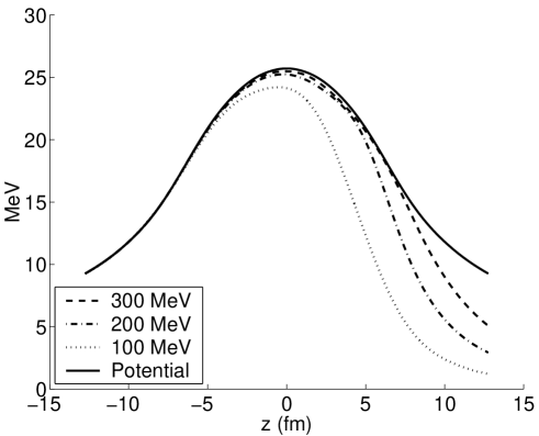
Figure 5: Comparison of (derivatives of) the phase of electron wave functions along the $z-$axis for electrons incident on a ²⁰⁸Pb nucleus with different energies.

2.2 EMA from DWBA

We establish now a connection between the DWBA results and the EMA. The DWBA transition amplitude for high momentum transfer in inelastic electron scattering can be written for one-photon exchange as

$$T_{if}=\int d^{3}r_{e}d^{3}r_{N}\Bigl{\{}\rho_{e}(\vec{r}_{e})\rho_{if}(\vec{r}_{N})-\vec{j}_{e}(\vec{r}_{e})\vec{J}_{if}(\vec{r}_{N})\Bigr{\}}\frac{e^{i\omega r}}{|\vec{r}_{e}-\vec{r}_{N}|}$$ (18)

with $\rho_{e},\,\rho_{if},\,\vec{j}_{e},\,\vec{J}_{if}$ being the charge and current densities of the electron and the nucleus, respectively, and $\omega$ is the energy loss of the electron. The double volume integral presents a clear numerical disadvantage of this expression. According to Knoll [39], one may introduce the scalar operator

$$S=e^{i\vec{q}\vec{r}}\sum\limits_{n=0}\Biggl{(}\frac{2i\vec{q}\,\vec{\nabla}+\Delta}{\vec{q}^{\,2}-\omega^{2}}\Biggr{)}^{n}e^{-i\vec{q}\vec{r}},\quad\vec{q}=\vec{k}_{i}-\vec{k}_{f},$$ (19)

such that the transition amplitude can be expanded in a more convenient form ($Q^{2}=\vec{q}^{\,2}-\omega^{2}$)

$$T_{if}=\frac{4\pi}{Q^{2}}\int d^{3}r\Bigl{[}\rho_{if}(\vec{r})S\rho_{e}(\vec{r})-\vec{J}_{if}S\vec{j}_{e}(\vec{r})\Bigr{]}.$$ (20)

The single integral is limited to the region of the nucleus, where the nuclear current is relevant. The expansion (19) is an asymptotic one, which means that there is an optimum number (depending on $\vec{q}$) of terms that give the best approximation to the exact value. Considering terms up to second order in the derivatives only one obtains

$$T_{if}=\frac{4\pi}{Q^{2}}\int d^{3}r\Biggl{\{}\rho_{if}(\vec{r})e^{i\vec{q}\vec{r}}\Biggl{[}1+\frac{2i\vec{q}\,\vec{\nabla}+\Delta}{Q^{2}}-\frac{4(\vec{q}\,\vec{\nabla})^{2}}{(Q^{2})^{2}}\Biggr{]}e^{-i\vec{q}\vec{r}}\rho_{e}(\vec{r})+\mbox{current terms}\Biggr{\}}.$$ (21)

Note that the $e^{-i\vec{q}\vec{r}}$-term in front of the electron charge or current density cancels the spatial oscillatory behavior of the densities in the asymptotic region far from the nucleus, such that the gradient operator $\vec{\nabla}$ in eq. (21) probes only the distortion of the electron current due to the nuclear Coulomb potential. Therefore, eq. (21) provides a satisfactory approximation for many interesting cases when $Q^{2}\gg q\Delta k$ is fulfilled. E.g., for a typical initial electron energy $\epsilon_{i}=400$ MeV used in inclusive quasielastic electron scattering experiments and energy transfer $\omega=\epsilon_{i}-\epsilon_{f}=100$ MeV, the contribution to the cross section due to the $(\vec{q}\,\vec{\nabla})^{2}$-term in eq. (21) is only of the order of 2% for momentum transfer $q\geq 350$ MeV [8, 25].

Expansion (21) allows for a clear comparison of the plane wave Born approximation, the EMA and the DWBA. The effect of the electrostatic nuclear field on the matrix element $T_{if}$ is obviously given by a modification of the free electron charge and current densities $\rho_{e}$, $\vec{j}_{e}$ via the replacements

$$[\rho_{e}(\vec{r}),\vec{j}_{e}(\vec{r})]\rightarrow[\rho_{e}^{\prime}(\vec{r}),\vec{j}_{e}^{\prime}(\vec{r})]=e^{i\vec{q}\vec{r}}\Biggl{[}1+\frac{2i\vec{q}\,\vec{\nabla}+\Delta}{Q^{2}}-\frac{4(\vec{q}\,\vec{\nabla})^{2}}{(Q^{2})^{2}}\Biggr{]}e^{-i\vec{q}\vec{r}}[\rho_{e}(\vec{r}),\vec{j}_{e}(\vec{r})].$$ (22)

Having exact wave functions at hand, it is possible to perform a numerical analysis of this modification. For this purpose, it is advantageous to introduce the effective four-momentum transfer squared given by $Q^{\prime 2}=(\vec{k}_{i}^{\prime}-\vec{k}_{f}^{\prime})^{2}-\omega^{2}$. Then a short calculation shows that ($\epsilon_{i,f}\gg m$)

$$\frac{Q^{\prime 2}}{Q^{2}}=\frac{k_{i}^{\prime}k_{f}^{\prime}}{k_{i}k_{f}},$$ (23)

i.e., when cross sections are calculated using the EMA, the enhanced photon propagator appearing in the matrix element $T_{if}$ exactly cancels the focusing effect of the initial and final state wave function. A numerical analysis shows that this is indeed also true for the DWBA case to a high degree of accuracy. E.g., a calculation for relatively low electron energies $\epsilon_{i}=300$ MeV, $\epsilon_{f}=200$ MeV and scattering angle $\vartheta_{e}=60^{o}$ of

$$\bar{f^{\prime}}^{2}=\frac{\int d^{3}r|\rho_{e}^{\prime}(\vec{r})|\rho(\vec{r})}{\int d^{3}r\rho(\vec{r})},\quad\bar{f}^{2}_{\mbox{\footnotesize{free}}}=\frac{\int d^{3}r|\rho_{e}^{\mbox{\footnotesize{free}}}(\vec{r})|\rho(\vec{r})}{\int d^{3}r\rho(\vec{r})}$$ (24)

in analogy to eq. (9) leads for ²⁰⁸Pb to the numerical result $\bar{f^{\prime}}^{2}/\bar{f}^{2}_{\mbox{\footnotesize{free}}}=0.985$, i.e. the wave function focusing effect of $\sim 17\%$ in the electron charge density is in fact overcompensated slightly by $\sim 1.5\%$ compared to the free plane wave charge density due to the enhanced momentum transfer. The situation is similar for a backscattering angle $\vartheta_{e}=143^{o}$, which has also been used in the experiment [36]. Numerical calculations reveal that the same observation applies to the components of the current density. Defining focusing factors $\bar{f^{\prime}}^{2}_{k}$ for each current component $\vec{j}_{e}=(j_{x},j_{y},j_{z})$ again leads to the result that the effect of the $S$-operator is just a cancellation of the average focusing effect in the initial and final state wave functions.

Finally, we investigated the modification of the momentum transfer inside the nucleus. For this purpose, we defined the local momentum transfer $\vec{q}(\vec{r})$ according to

$$\rho_{e}^{\prime}(\vec{r})=|\rho_{e}^{\prime}(\vec{r})|e^{i\vec{q}(\vec{r})\vec{r}}$$ (25)

and calculated the quantities

$$q_{1}^{\prime}=\frac{\int d^{3}r|\vec{q}(\vec{r})|\rho(\vec{r})}{\int d^{3}r\rho(\vec{r})},\quad{q^{\prime}}_{\,2}^{2}=\frac{\int d^{3}r|\vec{q}(\vec{r})|^{2}\rho(\vec{r})}{\int d^{3}r\rho(\vec{r})}$$ (26)

The results for $q_{1}^{\prime}$ and $q_{2}^{\prime}$ are again compatible with an average potential of $20$ MeV. Replacing $\rho_{e}^{\prime}$ by $\rho_{e}$ in eq. (25) has nearly no influence on the result for the corresponding effective momenta $q_{1}$ and $q2$, and again the situation is completely analogous for the current density.

2.3 Coulomb corrections for a harmonic oscillator single particle shell model

We point out that the discussion presented above is a most general one as long as detailed properties of the nuclear current are ignored. The hope is of course that the presence of, e.g., 208 nucleons in a ²⁰⁸Pb nucleus leads to a smooth nucleon momentum distribution, such that the features of the individual nucleon wave functions are averaged out to some degree in the momentum regime relevant for our discussion. Calculations in the framework of the eikonal approximation as presented in [25], but with the electron amplitudes adapted to the amplitudes from exact calculations, also agree well with the EMA, a fact which supports the assumption that a semiclassical description of Coulomb corrections can be found at high momentum transfer. Still, one cannot exclude from the first that the semiclassical picture of the transition amplitude which has been presented in the previous discussion is flawed by phase effects which enter the cross section, leading to unexpected deviations from the idealized EMA-behavior.

We therefore present results for a Pb model nucleus consisting of 82 scalar protons with harmonic nucleon wave functions for some typical kinematical situations, which indeed show that the modified EMA, using an average potential value, reproduces the Coulomb effects with high accuracy for $(e,e^{\prime})$ scattering, if the momentum transfer and the energy of the outgoing electron are high enough. The smaller contribution of the neutrons was neglected in the calculations, since we will focus on general considerations in the following. A detailed study using relativistic nucleon wave functions including spin in conjunction with more realistic current models will be presented in detail in a forthcoming paper.

At the lowest energies that have been used in the positron experiment by Guèye et al. [35], i.e., for an initial electron energy $\epsilon_{i}^{-}=224$ MeV and initial positron energy $\epsilon_{i}^{+}=262$ MeV, the situation is a bit more involved, and we found a relatively large disagreement between the exact inclusive cross sections and the values calculated from the EMA with an effective potential value of $19$ MeV, as will be demonstrated below. This observation is not astonishing, since the typical energy of the outgoing electrons is only of the order of $100$ MeV in this case (see also Fig. 5).

The radial wave function $R_{nl}$ of a particle in the harmonic oscillator shell model potential $V(r)=-v_{0}+\frac{1}{2}M\omega_{o}^{2}r^{2}$, where $M$ is the proton mass, is given by ($n=1,2...$ and $l=0,1...)$

$$R_{nl}(r)=\frac{1}{\sqrt{x_{o}^{3}}}N_{nl}\Biggl{(}\frac{r^{l}}{x_{o}^{l}}\Biggr{)}L_{n-1}^{l+\frac{1}{2}}\Biggl{(}\frac{r^{2}}{x_{o}^{2}}\Biggr{)}e^{-\frac{1}{2}\frac{r^{2}}{x_{o}^{2}}},\quad x_{o}^{2}=\frac{\hbar}{M\omega_{o}}$$ (27)

such that $R_{nl}$ fulfills the normalization condition $\int_{0}^{\infty}R_{nl}^{2}(r)\,r^{2}\,dr=1$ and the integral $\langle n\,l|r^{2}|n\,l\rangle$ has the value $(N=2n+l-2)$

$$\langle r^{2}\rangle=\int_{0}^{\infty}R_{nl}^{2}(r)\,r^{4}\,dr=x_{o}^{2}(N+\frac{3}{2}),$$ (28)

with normalization constants

$$N_{nl}^{2}=\frac{2^{n+l+1}}{\sqrt{\pi}(n-1)!(2n+2l-1)!!}.$$ (29)

The Legendre polynomials are given by

$$L_{n-1}^{l+\frac{1}{2}}(z)=\sum_{k=0}^{n-1}\frac{(-1)^{k}}{2^{n-k-1}}{n-1\choose k}\frac{(2n+2l-1)!!}{(2l+2k+1)!!}z^{k}$$ (30)

and the energies are $E_{N}=-v_{0}+\hbar\omega_{o}(N+3/2)$. A popular phenomenological choice for the oscillator strength is $\hbar\omega_{o}\sim 41\,\mbox{MeV}\,A^{-1/3}$. The $(n,l)=(1,5)$-shell corresponds to the $1h_{11/2}$-shell in the spin-orbit interaction model and contains 12 protons (but $2(2l+1)=22$ available states, when an artificial spin factor of $2$ is included), whereas the the $(n,l)=(1,0)$, $(2,0$), $(3,0)$, $(1,1)$, $(1,2)$, $(2,1)$, $(2,2)$, $(1,3)$, and $(1,4)$-shell are fully occupied. We therefore assumed for the calculation of cross sections that the $(1,5)$-shell is completely filled, i.e. spherically symmetric, and adopted a weighting factor of $12/22$ leading to an rms charge radius of the Pb model nucleus of $r_{{}_{rms}}=\sqrt{393/82}x_{0}$, as can be derived from eq. (28). Accordingly, $x_{o}=2.515$ fm was used in the calculations, such that the rms charge radius for the nucleus adds up to $5.505$ fm.

The proton transition current density was calculated from the free form of the Klein-Gordon expression

$$\vec{j}_{p}=\frac{ie}{2M}\Bigl{\{}\Phi^{*}_{f}\vec{\nabla}\Phi_{nlm}-\Phi_{nlm}\vec{\nabla}\Phi^{*}_{f}\Bigr{\}}$$ (31)

for initial states $\Phi_{nlm}(\vec{r})=R_{nl}(r)Y_{lm}(\vec{r}/r)$ and final plane wave states $\Phi_{f}=e^{i\vec{k}_{f}^{p}\vec{r}}$. The transition charge density was calculated from the exact current conservation relation

$$i\omega j_{p}^{0}=\vec{\nabla}\vec{j}_{p},$$ (32)

where $\omega=\epsilon_{i}-\epsilon_{f}$ is the energy transferred to the proton as defined before. The model used for the proton current is simple, but it has the advantage that it allows to perform analytical calculations for the electron plane wave case, which permit a verification of the accuracy of the numerical calculations. It also captures the most important features of the $(e,e^{\prime})$ cross sections in the vicinity of the quasielastic peak. Furthermore, it has to be pointed out that the Ohio group used a single particle shell model, where the nucleon wave functions were obtained by solving the Dirac equation for each shell nucleon with phenomenological S-V-potentials. But a comparison of measured data and calculations shows large discrepancies especially at higher energy transfer $\omega\geq 150$ MeV, where correlation effects and pion production become increasingly important. Therefore also a single particle shell model with ‘exact’ nucleon wave functions cannot be considered as an ‘exact’ model for inclusive quasielastic scattering. Hence, the optimal strategy is to find a general, model independent method which makes it possible to include the Coulomb distortion effect in the analysis of experimental data.

For lower electron energies, where the EMA cross sections ($\sigma_{{}_{EMA}}$) start to deviate significantly from the exact ones ($\sigma_{{}_{CC}}$), it is still possible to match the EMA and exact cross sections by using an effective potential value $\bar{V}_{fit}$ that differs from the commonly used $18-20$ MeV for Pb. E.g., for $\epsilon_{i}^{-}=224$ MeV, $\sigma_{{}_{CC}}$ and $\sigma_{{}_{EMA}}$ are very close for $\bar{V}_{fit}\sim 27$ MeV in our model for an energy transfer larger than $100$ MeV. This effective value is very stable under distortions of the scalar proton current model; using a ‘wrong’ value for $\omega$ in eq. (32) which is $20$ MeV larger or smaller than $\epsilon_{i}-\epsilon_{f}$ or including a potential term of similar order in eq. (31) changes the cross sections, but the effective potential value does not change significantly. This is a positive result, since it shows that our general considerations are not too strongly model dependent. Binding energies, nuclear potentials and the corresponding exact nucleon wave functions are relevant for an accurate modelling of amplitude, width and position of the quasielastic peak, but the impact of the Coulomb distortion of electrons on the quasielastic cross section expressed by a fitted effective potential $\bar{V}_{fit}$ can also be studied to some level using a simplified model with a quasielastic peak that incorporates approximately the properties of the true quasielastic cross section. Since binding energies are indeed neglected in our theoretical model, a shift of the quasielastic peak by about $25$ MeV to lower energy transfer is observed.

It is very instructive to investigate the total response function $S^{tot}$, which is defined in plane wave Born approximation by

$$\frac{d^{2}\sigma_{{}_{PWBA}}}{d\Omega_{f}d\epsilon_{f}}=\sigma_{Mott}\times S^{tot}_{{}_{PWBA}}(|\vec{q}\,|,\omega,\Theta),$$ (33)

via the well-known Mott cross section

$$\sigma_{Mott}=4\alpha^{2}\cos^{2}(\Theta/2)\epsilon_{f}^{2}/Q^{4}$$ (34)

not only for the total cross section, but also for individual filled shells. According to eq. (23), the Mott cross section remains unchanged when it gets multiplied by the EMA focusing factors and the momentum transfer $Q^{4}$ is replaced by its corresponding effective value. Therefore, if the EMA is a good approximation, the cross section can be written (see also [35])

$$\frac{d^{2}\sigma_{{}_{CC}}}{d\Omega_{f}d\epsilon_{f}}\simeq\frac{d^{2}\sigma_{{}_{EMA}}}{d\Omega_{f}d\epsilon_{f}}=\sigma_{Mott}\times S^{tot}_{{}_{PWBA}}(|\vec{q}_{{}_{eff}}|,\omega,\Theta).$$ (35)

Table 1 shows ratios of total responses, which have been obtained by dividing the same Mott cross section out of the inclusive Coulomb corrected, EMA-, and PWBA-cross sections restricted to single closed shells. The first two columns show a case where both the initial and final electron energy is larger than $300$ MeV, the other four columns show two kinematical settings where both the initial and final electron (positron) energy is smaller than $300$ MeV. In all three cases, an effective potential value of $19$ MeV was used.

It is an interesting point is that even closed shells show an EMA-like behavior at higher electron energy. This is indeed not the case for single states, which are not spherically symmetric. Summing over all shells, one obtains a ratio $S^{tot}_{{}_{CC}}/S^{tot}_{{}_{EMA}}$ which is practically one for an effective potential value $\bar{V}=19$ MeV in the case where $\epsilon_{i}=485$ MeV. Note that the different shells contribute differently to the total cross section, according to the number of protons contained in them and their momentum distribution. E.g., the (1,0)-shell, which show the most irregular behavior for the kinematics shown in Table 1 due to its narrow momentum distribution, contributes only marginally to the total cross section because the shell contains only 2 protons.

In the case given in Table 1 with an initial electron energy $\epsilon_{i}^{-}=224$ MeV, the exact cross section is $7.3\%$ larger than the EMA cross section and $24.4\%$ larger than the plane wave cross section. By naive interpolation, one can infer that the exact and the EMA cross section should be identical for an effective potential value which is larger than $19$ MeV. This indeed the case for an approximate value $\bar{V}_{fit}\simeq 27$ MeV, and similarly in the positron case for $\bar{V}_{fit}\simeq 25$ MeV. The maximum values of the total response for the $\epsilon_{i}^{-}=224$ MeV and $\epsilon_{i}^{+}=262$ MeV case differ by about $10\%$, i.e., one observes a relatively large deviation from the EMA prediction that the two responses agree. However, for higher energies used in the positron experiment of Guèye et al., an effective potential value of $18.9\pm 1.5$ MeV is compatible with our model calculations.

The accuracy concerning the calculation of cross sections and accordingly the values given in Table 1 is limited to about $1\%$ due to the truncation of the Knoll expansion eq. (21) and the finite resolution of the grid that has been used for the modelling of the nucleus. The numerical evaluation of transition amplitudes was performed by putting the nucleus on a three dimensional cubic grid with a side length of $30$ fm and a grid spacing of $(30/140)$ fm, and convergence was checked by using different side lengths and grid resolutions. The accuracy of the solid angle integration of the $(e,e^{\prime}p)$ cross section was better than $0.05\%$.

$(n,l)$	$S^{tot,nl}_{{}_{CC}}/S^{tot,nl}_{{}_{\!EMA}}$	$\!S^{tot,nl}_{{}_{CC}}/S^{tot,nl}_{{}_{\!PWBA}}$	$S^{tot,nl}_{{}_{CC}}/S^{tot,nl}_{{}_{\!EMA}}$	$\!S^{tot,nl}_{{}_{CC}}/S^{tot,nl}_{{}_{\!PWBA}}$	$S^{tot,nl}_{{}_{CC}}/S^{tot,nl}_{{}_{\!EMA}}$	$\!S^{tot,nl}_{{}_{CC}}/S^{tot,nl}_{{}_{\!PWBA}}$
(1,0)	1.101	1.811	1.275	3.574	0.776	0.425
(2,0)	1.004	0.971	0.996	0.972	1.056	0.679
(3,0)	1.013	1.046	1.116	1.272	1.033	0.870
(1,1)	1.024	1.332	1.140	2.041	0.896	0.758
(1,2)	0.989	1.094	1.063	1.384	0.964	0.982
(2,1)	1.013	1.268	1.050	1.377	1.025	0.718
(2,2)	0.995	1.271	1.031	1.526	1.028	0.939
(1,3)	0.982	0.989	1.054	1.132	1.003	1.087
(1,4)	0.990	0.956	1.072	1.043	1.011	1.115
(1,5)	1.005	0.955	1.085	1.011	1.006	1.117
$\sum\limits_{\,(n,l)^{\prime}}$	0.999	1.072	1.073	1.244	0.989	0.956

Table 1: Ratio of the total response for different filled shells, calculated in plane wave approximation ($S^{tot}_{{}_{PWBA}}$) and EMA with an effective potential $19$ MeV ($S^{tot}_{{}_{EMA}}$), with the exact response $S^{tot}_{{}_{CC}}$. First two columns: Initial electron energy $\epsilon_{i}=485$ MeV, $\omega=140$ MeV, $\vartheta_{e}=60^{o}$. Columns 3 & 4: Initial electron energy $\epsilon_{i}=224$ MeV, $\omega=100$ MeV, $\vartheta_{e}=143^{o}$. Columns 5 & 6: Initial positron energy $\epsilon_{i}=262$ MeV, $\omega=100$ MeV, $\vartheta_{p}=143^{o}$. The bottom line shows the ratios of the total response functions for the full cross sections, i.e. after summing over all shells with a weighting factor 6/11 for the (1,5)-shell. Note that these values are not averages of the data in the column above, since the contribution of each shell to the total cross section is different.

3 Conclusions

The complex behavior of the Coulomb distortion of electron waves at relatively high energies relevant for quasielastic electron-nucleus scattering experiments was studied using accurate numerical calculations. Naive lowest order approximations in $\alpha Z$ are not suitable for the analysis of Coulomb corrections in scattering experiments, unless they are modified in a well-controlled manner based on exact calculations. A Fortran 90 program is available now which can be used for accurate calculations of continuum electron wave functions in a central electrostatic field. The exact wave functions were used for a numerical study of Coulomb distortions in inclusive quasielastic electron scattering. It turns out that the effective momentum approximation is not reliable when the central potential value $V_{0}$ of the electrostatic field of the nucleus is taken as basis for the EMA calculations, but a smaller average value $\bar{V}\sim(0.75...0.8)V_{0}$ leads to very good results, if the momentum transfer and the energy of the scattered electron large enough. An effective potential value of $19$ MeV is a very good choice for $\epsilon_{f}\geq 300$ MeV and $Q^{2}\geq(400\,\mbox{MeV})^{2}$, and we conjecture that at very high energies, a limiting effective potential value close to $20$ MeV is reached. If the energy of the scattered electron becomes smaller than $300$ MeV, the semiclassical description of the final state wave function becomes obsolete, but it is still possible to use an EMA-like approach for the description of the inclusive cross section by using a modified fitted potential value, given the condition that the initial and final energy of the electron and the momentum transfer are not too small. In this region, detailed calculations become necessary with more refined nuclear models that the one used in this work. However, for the kinematical settings that will be used in the future experiments at the TJNAF, our analysis shows that the EMA will provide a valuable strategy for the correction of data.

It highly improbable that the match of our exact cross sections with the EMA cross sections (i.e., with $\bar{V}=20$ MeV for ²⁰⁸Pb), which is better than $2\%$ for the kinematical region $\epsilon_{f}\geq 300$ MeV and $Q^{2}\geq(400\,\mbox{MeV})^{2}$, is just a pure coincidence, since both approaches are unrelated and based on different calculational strategies. We must therefore conclude that our findings are not compatible with the conclusions drawn in [8].

Appendix: Calculation of continuum states of an electron in a central electrostatic field

Some details concerning the description of electron continuum states in a central electrostatic field are given here for the reader’s convenience and in order to give a fully consistent description of the problem.

We first consider the solutions of the stationary Dirac equation

$$[-i\vec{\alpha}\vec{\nabla}+m\beta+V(\vec{r})]\psi(\vec{r})=E\psi(\vec{r})$$ (36)

for an electron with total energy $E$ subject to the central electrostatic potential generated by a spherically symmetric nucleus with charge number $Z$. We use standard Dirac and Pauli matrices [40]. Dirac spinors describing states with definite angular momentum and parity can be decomposed into a radial and an angular part

$$\psi_{\kappa}^{\mu}=\left(\begin{array}[]{c}g_{\kappa}(r)\chi_{\kappa}^{\mu}(\hat{\bf{r}})\\ if_{\kappa}(r)\chi_{-\kappa}^{\mu}(\hat{\bf{r}})\end{array}\right)$$ (37)

with two-component spinors $\chi_{\kappa}^{\mu}$ which are eigenstates of the spin-orbit operator

$$(\vec{\sigma}\vec{L}+1)\chi_{\kappa}^{\mu}=-\kappa\chi_{\kappa}^{\mu}$$ (38)

and the angular momentum operators

$$\vec{J}^{\,2}\chi_{\kappa}^{\mu}=(\vec{L}+\vec{s}\,)^{2}\chi_{\kappa}^{\mu}=j(j+1)\chi_{\kappa}^{\mu},$$

$$\vec{L}^{2}\chi_{\kappa}^{\mu}=l(l+1)\chi_{\kappa}^{\mu}\,,\quad\vec{s}^{\,2}\chi_{\kappa}^{\mu}=\frac{3}{4}\chi_{\kappa}^{\mu},$$

$$J_{z}\chi_{\kappa}^{\mu}=\mu\chi_{\kappa}^{\mu}\,,$$ (39)

where $\kappa=\pm 1,\pm 2,...$ is related to $j$ and $l$ by

$$\kappa=l(l+1)-(j+\frac{1}{2})^{2},\quad j=|\kappa|-\frac{1}{2},\quad l=j+\frac{1}{2}\mbox{sgn}(\kappa),$$ (40)

and the operators $\vec{L}$ and $\vec{s}$ are given by $\vec{L}=-i\vec{r}\times\vec{\nabla}$ and $\vec{s}=\frac{1}{2}\vec{\sigma}$. The spinors can be expressed using Clebsch-Gordan coefficients as

$$\chi_{\kappa}^{\mu}=\sum_{\zeta=\pm 1/2}\langle l(\mu-\zeta)\frac{1}{2}\zeta|j\mu\rangle Y_{l}^{\mu-\zeta}({\bf\hat{r}})\chi_{\zeta},\quad\hat{j}=\sqrt{2j+1}$$ (41)

where $\chi_{\zeta}$ are standard Pauli spinors, or more explicitly

$$\chi_{\kappa}^{\mu}=\left(\begin{array}[]{c}\sqrt{\frac{j+\mu}{2j}}Y_{l,\mu-\frac{1}{2}}\\ \sqrt{\frac{j-\mu}{2j}}Y_{l,\mu+\frac{1}{2}}\end{array}\right)\,\,\mbox{for}\,\,\kappa<0,\quad\chi_{\kappa}^{\mu}=\left(\begin{array}[]{c}-\sqrt{\frac{j-\mu+1}{2j+2}}Y_{l,\mu-\frac{1}{2}}\\ \sqrt{\frac{j+\mu+1}{2j+2}}Y_{l,\mu+\frac{1}{2}}\end{array}\right)\,\,\mbox{for}\,\,\kappa>0.$$ (42)

The radial functions $f_{\kappa}$ and $g_{\kappa}$ fulfill the coupled differential equations

$$\frac{d}{dr}\left(\begin{array}[]{c}g_{\kappa}\\ f_{\kappa}\end{array}\right)=\left(\begin{array}[]{cc}-\frac{\kappa+1}{r}&E+m-V\\ -(E-m-V)&\frac{\kappa-1}{r}\end{array}\right)\left(\begin{array}[]{c}g_{\kappa}\\ f_{\kappa}\end{array}\right)\,.$$ (43)

For an electron with energy $E>0$ in the Coulomb field of a point like charge $eZ$ the potential $V$ is

$$V(r)=-\xi/r,\quad\xi=\alpha Z,$$ (44)

and the continuum solutions of the Dirac equation are given by (see [41] and references therein)

$$\left(\begin{array}[]{c}g_{\kappa}\\ f_{\kappa}\end{array}\right) = \left(\begin{array}[]{c}1\\ -\sqrt{\frac{E-m}{E+m}}\end{array}\right)(kr)^{\gamma_{\kappa}-1}\frac{2^{\gamma_{\kappa}}e^{\pi\eta/2}\mid\Gamma(\gamma_{\kappa}+i\eta)\mid}{\Gamma(2\gamma_{\kappa}+1)}$$ (52)

$$\left(\begin{array}[]{c}\mbox{Re}\\ \mbox{Im}\end{array}\right)[(\gamma_{\kappa}+i\eta)e^{i\varphi}e^{-ikr}F(\gamma_{\kappa}+1+i\eta,2\gamma_{\kappa}+1;2ikr)],$$

where

$$\gamma_{\kappa}=\sqrt{\kappa^{2}-\xi^{2}}\quad,\quad\eta=\frac{\xi E}{k},$$

$$e^{2i\varphi}=\frac{-\kappa+i\eta m/E}{\gamma_{\kappa}+i\eta}\quad,\quad k=\sqrt{E^{2}-m^{2}}.$$ (53)

$\varphi$ is positive for $\mbox{arg}\,e^{2i\varphi}\in[0,\pi]$ and negative for $\mbox{arg}\,e^{2i\varphi}\in(-\pi,0]$. These Coulomb wave functions have the asymptotic forms ($r\rightarrow\infty$)

$$g_{\kappa}(r)\sim\frac{1}{kr}\cos(kr+\eta\log 2kr-(l+1)\frac{\pi}{2}+\delta_{\kappa})\,,$$ (54)

$$f_{\kappa}(r)\sim-\sqrt{\frac{E-m}{E+m}}\frac{1}{kr}\sin(kr+\eta\log 2kr-(l+1)\frac{\pi}{2}+\delta_{\kappa})\,,$$ (55)

where

$$\delta_{\kappa}=\frac{1}{2}\mbox{arg}\frac{-\kappa+\frac{i\eta m}{E}}{\gamma_{\kappa}+i\eta}-\mbox{arg}\,\Gamma(\gamma_{\kappa}+i\eta)-\gamma_{\kappa}\frac{\pi}{2}+(l+1)\frac{\pi}{2}:=$$

$$\varphi-\mbox{arg}\,\Gamma(\gamma+i\eta)+(l+1-\gamma)\frac{\pi}{2}.$$ (56)

In the limiting case $Z\rightarrow 0$, we have

$$g_{\kappa}(r)\rightarrow-\mbox{sgn}(\kappa)j_{l}(kr)\,,\quad f_{\kappa}(r)\rightarrow-\sqrt{\frac{E-m}{E+m}}j_{l^{\prime}}(kr),$$ (57)

where $j_{l}(kr)=\sqrt{\frac{\pi}{2kr}}J_{l+1/2}(kr)$ are spherical Bessel functions of the first kind, and $l^{\prime}=j-\frac{1}{2}\mbox{sgn}(\kappa)=l(-\kappa)$. Replacing $\gamma_{\kappa}$ by $-\gamma_{\kappa}$ in eq. (52) and correspondingly in eq. (53) leads to the irregular solutions $g_{\kappa}^{i}$, $f_{\kappa}^{i}$. Their asymptotic forms are also given by eqns. (54,55), if one replaces the expression for the phase shift $\delta_{\kappa}(\gamma_{\kappa})$ of the regular solutions by $\delta_{\kappa}^{\prime}(\gamma_{\kappa})=\delta_{\kappa}(-\gamma_{\kappa})$.

The calculation of the wave functions $g_{\kappa}$ and $f_{\kappa}$ is most simply performed by using the real series expansion

$$\left(\begin{array}[]{c}g_{\kappa}\\ f_{\kappa}\end{array}\right)=(kr)^{\gamma_{\kappa}-1}\sum_{n=0}^{\infty}\left(\begin{array}[]{c}a_{\kappa;n}\\ b_{\kappa;n}\end{array}\right)(kr)^{n}\,.$$ (58)

Inserting the series expansion (58) into eq. (43) leads to the coupled recursion relations [41]

$$(n+1)(2\gamma_{\kappa}+n+1)ka_{\kappa;n+1}+\xi(E-m)a_{\kappa;n}$$

$$-(\gamma_{\kappa}+n+1-\kappa)(E+m)b_{\kappa;n} = 0\,,$$ (59)

$$(n+1)(2\gamma_{\kappa}+n+1)kb_{\kappa;n+1}+\xi(E+m)b_{\kappa;n}$$

$$+(\gamma_{\kappa}+n+1+\kappa)(E-m)a_{\kappa;n} = 0\,.$$ (60)

The series expansion (58) can be shown to converge for all values of $r$.

We give here some details for the derivation of the recursion relations. From

$$\frac{d}{dr}g(r)=(E+m+\xi/r)f(r)-\frac{\kappa+1}{r}g(r)$$ (61)

one readily derives

$$(\gamma-1)(kr)^{\gamma-1}k\sum\limits_{n=1}^{\infty}a_{n}(kr)^{n-1}+(\gamma-1)(kr)^{\gamma-1}\frac{a_{0}}{r}+(kr)^{\gamma-1}k\sum\limits_{n=1}^{\infty}na_{n}(kr)^{n-1}=$$

$$(E+m)(kr)^{\gamma-1}\sum\limits_{n=0}^{\infty}b_{n}(kr)^{n}+\xi(kr)^{\gamma-1}k\sum\limits_{n=1}^{\infty}b_{n}(kr)^{n-1}+\xi(kr)^{\gamma-1}\frac{b_{0}}{r}$$

$$-(\kappa+1)(kr)^{\gamma-1}k\sum\limits_{n=1}^{\infty}a_{n}(kr)^{n-1}-(\kappa+1)(kr)^{\gamma-1}\frac{a_{0}}{r},$$ (62)

where we have omitted the index $\kappa$ for notational convenience. Comparing the lowest order terms $\sim r^{\gamma-2}$ immediately leads to the starting relation

$$b_{0}=\frac{\kappa+\gamma}{\xi}a_{0}=\frac{\xi}{\kappa-\gamma}a_{0}.$$ (63)

From

$$\frac{d}{dr}f(r)=-(E-m+\xi/r)g(r)+\frac{\kappa-1}{r}f(r)$$ (64)

one obtains

$$(\gamma-1)(kr)^{\gamma-1}k\sum\limits_{n=1}^{\infty}b_{n}(kr)^{n-1}+(\gamma-1)(kr)^{\gamma-1}\frac{b_{0}}{r}+(kr)^{\gamma-1}k\sum\limits_{n=1}^{\infty}nb_{n}(kr)^{n-1}=$$

$$-(E-m)(kr)^{\gamma-1}\sum\limits_{n=0}^{\infty}a_{n}(kr)^{n}-\xi(kr)^{\gamma-1}k\sum\limits_{n=1}^{\infty}a_{n}(kr)^{n-1}-\xi(kr)^{\gamma-1}\frac{a_{0}}{r}$$

$$+(\kappa-1)(kr)^{\gamma-1}k\sum\limits_{n=1}^{\infty}b_{n}(kr)^{n-1}+(\kappa-1)(kr)^{\gamma-1}\frac{b_{0}}{r}.$$ (65)

Comparing again the lowest order terms $\sim r^{\gamma-2}$ leads again to the starting relation (63). Taking into account the higher order terms $\sim(kr)^{\gamma-1}(kr)^{n-1}$ in eqns. (62,65) leads to

$$(\gamma-1)ka_{n}+nka_{n}-(E+m)b_{n-1}-\xi kb_{n}+(\kappa+1)ka_{n}=0\,$$ (66)

$$(\gamma-1)kb_{n}+nkb_{n}+(E-m)a_{n-1}+\xi ka_{n}-(\kappa-1)kb_{n}=0.$$ (67)

Replacing $b_{n}$ from eq. (66)

$$b_{n}=\frac{\gamma+\kappa+m}{\xi}a_{n}-\frac{E+m}{\xi k}b_{n-1}$$ (68)

in eq. (67) gives

$$n(2\gamma+n)ka_{n}+\xi(E-m)a_{n-1}-(\gamma+n-\kappa)(E+m)b_{n-1}=0,$$ (69)

which is equivalent to eq. (59). Recursion relation (60) is obtained analogously.

An incident (outgoing) electron with asymptotic momentum $\vec{k}$, energy $E$ and polarization $\tau$ is given by a linear combination of the $\psi_{\kappa}^{\mu}$

$$\psi_{\tau}=4\pi\sqrt{\frac{E+m}{2E}}\sum\limits_{\kappa\mu}e^{\pm i\delta_{\kappa}}i^{l}\langle l\,(\mu-\tau)\,\frac{1}{2}\,\tau\,|\,j\,\mu\rangle(Y_{l}^{\mu-\tau}(\hat{\bf{k}}))^{*}\psi_{\kappa}^{\mu}(\vec{r}).$$ (70)

It is instructive to consider, e.g., the first component of the Dirac spinor $\psi_{\tau}$ for an electron incident along the z-axis with spin in the same direction. Then, the term $(Y_{l}^{\mu-\tau}(\hat{\bf{k}})^{*}$ is only non-zero when $\mu=\tau=1/2$, and we have

$$Y_{l}^{0}(\vartheta,\varphi)=\sqrt{\frac{2l+1}{4\pi}}P_{l}(\cos\vartheta),\quad Y_{l}^{0}(\vartheta=0,\varphi=0)=\sqrt{\frac{2l+1}{4\pi}}$$ (71)

Therefore, the first component of $\psi_{\tau}$ is given by

$$\psi_{\tau}^{1}=\sqrt{\frac{E+m}{2E}}\sum\limits_{\kappa}(2l+1)e^{i\delta_{\kappa}}i^{l}\langle l\,0\,\frac{1}{2}\frac{1}{2}\,|\,j\,\frac{1}{2}\rangle^{2}g_{\kappa}(r)P_{l}(\cos\vartheta).$$ (72)

A straightforward calculation shows that

$$\langle l\,0\,\frac{1}{2}\frac{1}{2}\,|\,j\,\frac{1}{2}\rangle^{2}=\frac{\kappa}{2\kappa+1}.$$ (73)

Furthermore, the asymptotic behavior of $g_{\kappa}$ is given by

$$g_{\kappa}(r)\sim\frac{1}{kr}\cos(kr+\eta\log 2kr-\mbox{arg}\,\Gamma(\gamma+i\eta)+\frac{1}{2}\mbox{arg}\,\frac{-\kappa+i\eta m/E}{\gamma+i\eta}-\gamma\frac{\pi}{2}).$$ (74)

We consider now the limit $Z\rightarrow 0$ for this asymptotic expression. For $Z\rightarrow 0$ we have also $\eta\rightarrow 0$, i.e. $\mbox{arg}\,\Gamma(\gamma+i\eta)\rightarrow 0$ and $\gamma\rightarrow|\kappa|$. From

$$e^{2i\varphi}=\frac{-\kappa+i\eta m/E}{\gamma+i\eta}=\frac{-\kappa\gamma+\eta m/E}{\gamma^{2}+\eta^{2}}+i\frac{\eta\kappa+\eta m/E}{\gamma^{2}+\eta^{2}}$$ (75)

we see that the argument of $\varphi$ approaches $\pi/2$ for $\eta\rightarrow 0$ and $\kappa>0$, whereas for $\kappa<0$ we have $\varphi\rightarrow 0$.
This shows that the asymptotic behavior of the $g_{\kappa}$ for $Z\rightarrow 0$ is given by

$$g_{\kappa}(r)\sim\frac{1}{kr}\cos(kr-\frac{\pi l}{2}+\mbox{sgn}(\kappa)\frac{\pi}{2})=-\mbox{sgn}(\kappa)\sin(kr-\frac{\pi l}{2}),$$ (76)

in accordance with eq. (57) which states that the free-field solutions of $g_{\kappa}$ are given by $g_{\kappa}(r)=-\mbox{sgn}(\kappa)j_{l}(kr)$. Therefore, the terms in the expansion (72) for $\kappa>0$ become ($l=\kappa$, $\delta_{\kappa}\rightarrow\pi$)

$$-\sqrt{\frac{E+m}{2E}}\sum\limits_{\kappa>0}li^{l}e^{i\pi}\frac{1}{kr}j_{l}(kr)P_{l}(\cos\vartheta)$$ (77)

and for $\kappa<0$ ($l=-\kappa-1$, $\delta_{\kappa}\rightarrow 0$)

$$\sqrt{\frac{E+m}{2E}}\sum\limits_{\kappa<0}(l+1)i^{l}\frac{1}{kr}j_{l}(kr)P_{l}(\cos\vartheta),$$ (78)

i.e. we obtain the partial wave expansion of a plane wave, and the normalization is such that the full free spinor for arbitrary momentum $\vec{k}$ and helicity $\zeta$ is given by

$$u_{\tau}=\sqrt{\frac{E+m}{2E}}\left(\begin{array}[]{c}\chi_{\tau}\\ \frac{\vec{\sigma}\vec{k}}{E+m}\chi_{\tau}\end{array}\right).$$ (79)

For the case of a realistic nuclear electrostatic potential, analytic expression for the radial functions are no longer available. Therefore, we calculated the radial wave functions by numerical integration according to the method described in appendix 3 of [32]. Outside the nuclear charge distribution (i.e. for $r>14$ fm in our actual calculations), the electrostatic potential is a Coulomb potential, and therefore the radial functions $G_{\kappa}$ obtained from the numerical integration can be written as a linear combination of regular and irregular solutions of the Dirac equation with a Coulomb potential

$$G_{\kappa}=c_{\kappa}g_{\kappa}+d_{\kappa}g_{\kappa}^{i}.$$ (80)

Since the asymptotic behavior of the regular and irregular radial functions is given by

$$g_{\kappa}(r)=\frac{1}{kr}\sin(kr+\eta\log 2kr-l\frac{\pi}{2}+\delta_{\kappa})$$ (81)

$$g_{\kappa}^{i}(r)=\frac{1}{kr}\sin(kr+\eta\log 2kr-l\frac{\pi}{2}+\delta^{\prime}_{\kappa})$$

$$=\frac{1}{kr}\sin(kr+\eta\log 2kr-l\frac{\pi}{2}+\delta_{\kappa}+(\delta^{\prime}_{\kappa}-\delta_{\kappa})),$$ (82)

and the asymptotic behavior of $G_{\kappa}$ is described by the phase shift $\Delta_{\kappa}$ via

$$G_{\kappa}(r)\sim\frac{\lambda}{kr}\sin(z+\Delta_{\kappa})$$ (83)

with $z=kr+\eta\log 2kr-l\frac{\pi}{2}+\delta_{\kappa}$, such that we obtain for $\Delta_{\kappa}$

$$\lambda\sin(z+\Delta_{\kappa})=\lambda\sin(z)\cos(\Delta_{\kappa})+\lambda\sin(\Delta_{\kappa})\cos(z)$$

$$=c_{\kappa}\sin(z)+d_{\kappa}\sin(z+\delta^{\prime}_{\kappa}-\delta_{\kappa})$$

$$=c_{\kappa}\sin(z)+d_{\kappa}\sin(z)\cos(\delta^{\prime}_{\kappa}-\delta_{\kappa})+d_{\kappa}\sin(\delta^{\prime}_{\kappa}-\delta_{\kappa})\cos(z),$$ (84)

the relations

$$\lambda\cos{\Delta_{\kappa}}=c_{\kappa}+d_{\kappa}\cos(\delta^{\prime}_{\kappa}-\delta_{\kappa})\quad,\quad\lambda\sin(\Delta_{\kappa})=d_{\kappa}\sin(\delta^{\prime}_{\kappa}-\delta_{\kappa})$$ (85)

and therefore

$$\tan{\Delta_{\kappa}}=\frac{\sin(\delta^{\prime}_{\kappa}-\delta_{\kappa})}{c_{\kappa}/d_{\kappa}+\cos(\delta^{\prime}_{\kappa}-\delta_{\kappa})},$$ (86)

which fix uniquely the phase shift $e^{i\Delta_{\kappa}}$. The radial function $G_{\kappa}$ (and the corresponding $F_{\kappa}$ for the lower spinor components) obtained from the numerical integration procedure must subsequently be multiplied by a factor $\lambda^{-1}$, where

$$\lambda^{2}=(\lambda\cos{\Delta_{\kappa}})^{2}+(\lambda\sin{\Delta_{\kappa}})^{2}=(c_{\kappa}^{2}+d_{\kappa}^{2}+2c_{\kappa}d_{\kappa}\cos{\Delta_{\kappa}})$$ (87)

such that

$${\tilde{G}_{\kappa}}=\frac{1}{\lambda}G_{\kappa}(r)\sim\frac{1}{kr}\sin(kr+\Delta_{\kappa})$$ (88)

is correctly normalized.

The expansion for an incoming wave scattering off a spherically symmetric nuclear charge distribution is finally given by

$$\psi_{\tau}=4\pi\sqrt{\frac{E+m}{2E}}\sum\limits_{\kappa\mu}e^{i\delta_{\kappa}}e^{i\Delta_{\kappa}}i^{l}\langle l\,(\mu-\tau)\,\frac{1}{2}\,\tau\,|\,j\,\mu\rangle Y_{l}^{\mu-\tau*}(\hat{\bf{k}})\psi_{\kappa}^{\mu}(\vec{r}),$$ (89)

where $\psi_{\kappa}^{\mu}$ is defined according to eq. (37) with the radial functions $g_{\kappa}$ and $f_{\kappa}$ replaced by $\tilde{G}_{\kappa}$ and $\tilde{F}_{\kappa}$.

References

- [1] R. R. Whitney, I. Sick, J. R. Ficenec, R. D. Kephart, W. P. Trower, Phys. Rev. C9, (1974) 2230-2235.
- [2] O. Benhar, A. Fabrocini, S. Fantoni, I. Sick, Phys. Lett. B343, (1995) 47-52.
- [3] J. Jourdan, Nucl. Phys. A604, (1996) 117-160.
- [4] D. Day, J. S. McCarthy, T. W. Donnelly, I. Sick, Ann. Rev. Nucl. Part. Sci. 40, (1990) 357-410.
- [5] D. B. Day, J. S. McCarthy, Z. E. Meziani, R. C. Minehart, R. M. Sealock, S. T. Thornton, J. Jourdan, I. Sick, B. W. Filippone, R. D. McKeown, R. G. Milner, D. H. Potterveld, Z. Szalata, Phys. Rev. C40, (1989) 1011-1024.
- [6] Mini-Workshop on Coulomb Corrections, Thomas Jefferson National Accelerator Facility, March 28, 2005, and Joint Jefferson Lab/Institute for Nuclear Theory Workshop on Precision ElectroWeak Interactions, College of William and Mary, Williamsburg VA, August 15-17, 2005.
- [7] J. Morgenstern, Z.E. Meziani, Phys. Lett. B515, (2001) 269-275.
- [8] K.S. Kim, L.E. Wright, Y. Jin, D.W. Kosik, Phys. Rev. C54, (1996) 2515-2524.
- [9] J.M. Udias, J.R. Vignote, E. Moya de Guerra, A. Escuderos, J.A. Caballero, Recent developments in relativistic models for exclusive A(e,e’p)B reactions, Workshop on “e-m Induced Two-Hadron Emission”, Lund, June 13-16, 2001.
- [10] J.M. Udias, P. Sarriguren, E. Moya de Guerra, E. Garrido, J.A. Caballero, Phys. Rev. C48, (1993) 2731-2739.
- [11] G. Co’, J. Heisenberg, Phys. Lett. B197, (1987) 489-492.
- [12] Lenz F., Ph.D. thesis, Freiburg, Germany, 1971.
- [13] J. Knoll, Nucl. Phys. A223, (1974) 462-476.
- [14] C. Giusti, F.D. Pacati, Nucl. Phys. A473, (1987) 717-735.
- [15] F. Lenz, R. Rosenfelder, Nucl. Phys. A176, (1971) 513-525.
- [16] C. Giusti, F. D. Pacati, Nucl. Phys. A485, (1988) 461-480.
- [17] M. Traini, S. Turck-Chieze, A. Zghiche, Phys. Rev. C38, (1988) 2799-2812.
- [18] M. Traini, M. Covi, Nuovo Cim. A108, (1995) 723-736.
- [19] R. Rosenfelder, Annals Phys. 128, (1980) 188-240.
- [20] M. Levy, J. Sucher, Phys. Rev. 186, (1969) 1656-1670.
- [21] R.L. Sugar, R. Blankenbecler, Phys. Rev. 183, (1969) 1387-1396.
- [22] S.J. Wallace, Annals Phys. 78, (1973) 190-257.
- [23] S.J. Wallace, J.A. McNeil, Phys. Rev. D16, (1977) 3565-3580.
- [24] H. Abarbanel, C. Itzykson, Phys. Rev. Lett. 23, (1969) 53-56.
- [25] A. Aste, K. Hencken, J. Jourdan, I. Sick, D. Trautmann, Nucl. Phys. A743, (2004) 259-282.
- [26] A. Aste, J. Jourdan, Europhys. Lett. 67, (2004) 753-759.
- [27] D.R. Yennie, F.L. Boos, D.G. Ravenhall, Phys. Rev. 137, no. 4B, (1965) 882-903.
- [28] M. Traini, Nucl. Phys. A694, (2001) 325-336.
- [29] Y. Jin, D.S. Onley, L.E. Wright, Phys. Rec. C45, (1992) 1311-1320.
- [30] Y. Jin, D.S. Onley, L.E. Wright, Phys. Rev. C50, (1994) 168-176.
- [31] J. Jourdan, Workshop on Electron-Nucleus Scattering, eds. O. Benhar, A. Fabrocini, Edizioni ETS, Pisa, p. 319, 1997.
- [32] D. R. Yennie, D. G. Ravenhall, R. N. Wilson, Phys. Rev. 95, (1954) 500-512.
- [33] H. de Vries, C. W. de Jager, C. de Vries, At. Data Nucl. Data Tables 36, (1987) 495-536.
- [34] G. Fricke, C. Bernhardt, K. Heilig, L. A. Schaller, L. Schellenberg, E. B. Shera, C. W. de Jager, At. Data and Nucl. Data Tables 60, (1995) 177-285.
- [35] P. Guèye, M. Bernheim, J. F. Danel, J. E. Ducret, L. Lakéhal-Ayat, J. M. Le Goff, A. Magnon, C. Marchand, J. Morgenstern, J. Marroncle, P. Vernin, and A. Zghiche-Lakéhal-Ayat, Phys. Rev. C60, (1999) 044308.
- [36] A. Zghiche, J.F. Danel, M. Bernheim, M.K. Brussel, G.P. Capitani, E. De Sanctis, S. Frullani, F. Garibaldi, A. Gerard, J.M. Le Goff, A. Magnon, C. Marchand, Z.E. Meziani, J. Morgenstern, J. Picard, D. Reffay-Pikeroen, M. Traini, S. Turck-Chieze, P. Vernin, Nucl. Phys. A572, (1994) 513-559, Erratum ibid. A584, (1995) 757.
- [37] A. Aste, K. Hencken, D. Trautmann, Eur. Phys. J. A21, (2004) 161-167.
- [38] H. C. Pauli, U. Raff, Comp. Phys. Commun. 9, (1975) 392-407.
- [39] J. Knoll, Nucl. Phys. A201, (1973) 289-300.
- [40] J. D. Bjorken, S. D. Drell, Relativistic Quantum Fields, Mc Graw-Hill, New York, 1965.
- [41] D. Trautmann, G. Baur, F. Rösel, J. Phys. B: At. Mol. Phys. 16, (1983) 3005-3013.