Microscopic approach of fission dynamics
applied to fragment kinetic energy
and mass distributions in ²³⁸U

Abstract

The collective dynamics of low energy fission in ²³⁸U is described within a time-dependent formalism based on the Gaussian Overlap Approximation of the time-dependent Generator Coordinate Method. The intrinsic deformed configurations of the nucleus are determined from the self-consistent Hartree-Fock-Bogoliubov procedure employing the effective force D1S with constraints on the quadrupole and octupole moments. Fragment kinetic energy and mass distributions are calculated and compared with experimental evaluations. The effect of the collective dynamics along the fission paths and the influence of initial conditions on these distributions are analyzed and discussed.

I Introduction

Interest in fission has recently increased since it is proposed to be used in new applications, such as accelerator driven systems, new electro-nuclear cycles - thorium based fuel cycle -, and the next generation of exotic beam facilities. For these applications, there is an important need for fission cross-sections in a large range of excitation energies, and also for mass-charge fission fragment distributions. For instance, precise knowledge of production rates of secondary long-lived fission residues and of neutron-rich isotopes is crucial for designing and simulating these new facilities. It is worth pointing out that relevant measurements of mass and charge distributions have been performed recently. For instance the production of exotic nuclei has been measured from spallation reactions of 1 A GeV ²³⁸U projectiles on an hydrogen target Be03 and isotopic yields have been deduced for elements between ⁵⁸Ni and ¹⁶³Eu. Furthermore, thanks to secondary beam facilities, fission properties of 70 short-lived radioactive nuclei can be found in references Sc00 ; Be02 . Such a systematic analysis of the fission properties covers a wide region of the nuclide chart and the transition between single- and double-humped mass distributions has been observed with a triple-humped structure for ²²⁷Th. It is important to test the accuracy of the theoretical prediction using the data in order to gain confidence in its predictions when applied to widely extended domains such as fission of nuclei far from stability, and fission for a large range of excitation energies.
From a theoretical point of view, the description of fission process stands at the crossroads of many subjects in the forefront of research. Both static and dynamical properties of the fissionning system are required, namely: nuclear configurations far from equilibrium, the interplay of collective and intrinsic degrees of freedom, and the dynamics of large amplitude collective motion. Theoretical works generally focus on the static part of the fission. For instance, many studies have been devoted to multi-dimensional potential energy surfaces Mo00 ; Pa88 from which fission barriers are extracted and to nuclear configurations at scission and associated fragment distributions Wi76 ; Br88 . On the other hand there are very few dynamical studies of fission, although dynamical effects are expected to play an essential role in particular in the descent from saddle to scission. Fragment mass distributions have recently been obtained by solving the classical three-dimensional Langevin equations Ka01 . The influence of the mass asymmetry degree of freedom on the variance of the mass distribution has been highlighted. Two types of microscopic quantum dynamical calculations have also been performed in the past. First, in 1978 the time-dependent Hartree Fock method Ne78 has been applied to fission. Second, time-dependent calculations based on the Generator Coordinate method using Hartree-Fock-Bogoliubov states have been performed, and the most probable fission configuration of ²⁴⁰Pu has been analyzed Be84 . The present study is an extension of this pioneering work.
In the present work we have chosen to derive the collective dynamics of fission using a time-dependent formalism based on the Gaussian Overlap Approximation of the time-dependent Generator Coordinate (GC) theory. An alternate method could have been to first determine the stationary solutions of the GC equations within the relevant domain of generator coordinates with appropriate boundary conditions. The solutions of the time-dependent GC equations would then be expressed in a straightforward manner. However, the precise form of the boundary conditions to be used is difficult to obtain when more than one generator coordinate are employed. Applying a time-dependent method allows one to avoid this problem. The only input of the calculation is the collective wave function chosen at t=0. Spurious reflections of the time-dependent collective wave function on the edge of the finite domain are eliminated using a standard absorption technique as explained in Section III.
In this paper, we focus on low energy fission-fragment distributions of ²³⁸U, and also on several physical aspects that can be clearly analyzed in this even-even fissioning system. Let us recall that, at low energy, elongation and asymmetry degrees of freedom are among the most relevant ones and that the adiabatic assumption is to a large extent justified Wa91 . As we explain below, time evolution in the fission channel is described in terms of a wave function of Hill-Wheeler type. The latter is taken as a linear combination of Hartree-Fock-Bogoliubov (HFB) solutions characterized by the two collective degrees of freedom just mentioned. It is worth pointing out that this work relies only on the D1S effective interaction used at Bruyères-le-Châtel.
The calculation proceeds in two steps: the potential energy surface and the collective inertia are determined from the first well to scission and then, the dynamical treatment of fission is performed using an approximate Time Dependent Generator Coordinate Method (TDGCM). Potential energy surfaces and associated collective inertia tensors are calculated using the constrained Hartree-Fock-Bogoliubov approach with the D1S finite-range effective force DG80 ; Be91 . Fission wave functions at time zero are constructed from the quasi-stationary collective states in the first well. Their time evolution is calculated numerically by discretizing on a mesh a time-dependent Schrödinger-like equation. Mass distributions are derived from the flux of the wave function through scission at given A_H/A_L fragmentations.
The present work is organized as follows. The HFB formalism and the TDGCM method are presented in Section II and numerical procedures are detailed in section III. Section IV is devoted to the static results, where the potential energy surface and pairing correlations are discussed. A first estimate of kinetic energy and fragment mass distributions, obtained from a ”static” calculation at scission, are discussed. Mass distributions obtained from the full time-dependent calculations are presented in Section V, and the crucial role played by dynamical effects is analyzed.

II Formalism

In low energy fission the adiabatic hypothesis seems to be justified Wa91 and, therefore, collective and intrinsic degrees of freedom can be decoupled. Furthermore, we assume that the collective motion of the system can be described in terms of a few collective variables characterizing the shape evolution of the nucleus. In a self-consistent formalism these shapes can be generated by means of external fields represented by the operators:

$$\hat{Q}_{20}=\sqrt{\frac{16\pi}{5}}\sum_{i=1}^{A}r_{i}^{2}Y_{20}=\sum_{i=1}^{A}(2z_{i}^{2}-x_{i}^{2}-y_{i}^{2}),$$ (1)

and

$$\hat{Q}_{30}=\sqrt{\frac{4\pi}{7}}\sum_{i=1}^{A}r_{i}^{3}Y_{30}=\sum_{i=1}^{A}(z_{i}^{3}-\frac{3}{2}z_{i}(x_{i}^{2}+y_{i}^{2})).$$ (2)

These moments govern mass axial deformation and left-right asymmetry of the nucleus, respectively. For well-separated fragments one can express the mean values of these operators in terms of $<Q_{20}^{H}>$ ($<Q_{30}^{H}>$) and $<Q_{20}^{L}>$ ($<Q_{30}^{L}>$), the mean quadrupole (octupole) deformations of the heavy and light fragments, respectively, $d_{m}$ the distance between their centers of mass, and $\mu$ the reduced mass :

$$\begin{array}[]{lll}<Q_{20}>&=&\displaystyle<Q_{20}^{H}>+<Q_{20}^{L}>+2\mu d_{m}^{2}\ ,\\ &&\\ <Q_{30}>&=&<Q_{30}^{H}>+<Q_{30}^{L}>\\ &&\displaystyle+\frac{3d_{m}}{A_{H}+A_{L}}(A_{H}<Q_{20}^{L}>-A_{L}<Q_{20}^{H}>)\\ &&\displaystyle+2\mu d_{m}^{3}\frac{A_{H}-A_{L}}{A_{H}+A_{L}}\ ,\end{array}$$ (3)

with

$$\mu=\frac{A_{H}A_{L}}{A_{H}+A_{L}}.$$ (4)

Relations (3) and (4) have only been used in the present work to check the validity of the computer program for configurations close to scission.
The intrinsic axially-deformed states ${|{\Phi(q_{20},q_{30})}\rangle}$ of the fissile system are taken as the solutions of the constrained Hartree-Fock-Bogoliubov variational principle Be91 :

$$\delta{\langle{\Phi(q_{20},q_{30})}}|\hat{H}-\lambda_{N}\hat{N}-\lambda_{Z}\hat{Z}-\sum_{i}\lambda_{i}\hat{Q}_{i}{|{\Phi(q_{20},q_{30})}\rangle}=0\ ,$$ (5)

the Lagrange parameters $\lambda_{N}$, $\lambda_{Z}$, and $\lambda_{i}$ being deduced from:

$${\langle{\Phi(q_{20},q_{30})}}|\hat{N}{|{\Phi(q_{20},q_{30})}\rangle}=N,$$

$${\langle{\Phi(q_{20},q_{30})}}|\hat{Z}{|{\Phi(q_{20},q_{30})}\rangle}=Z,$$ (6)

and

$${\langle{\Phi(q_{20},q_{30})}}|\hat{Q}_{i}{|{\Phi(q_{20},q_{30})}\rangle}=q_{i}.$$

In Eq. (5), $\hat{Q}_{i}$ is the set of external field operators ($\hat{Q}_{20}$, $\hat{Q}_{30}$, $\hat{Q}_{10}$), and $\hat{H}$ is the nuclear many-body effective Hamiltonian built with the finite-range effective force D1S Be91 . The additional constraint on the dipole mass operator is used in order to fix the position of the center of mass of the whole system. This is accomplished by setting $<\hat{Q}_{10}>$ = 0, where:

$$\begin{array}[]{llll}\displaystyle\hat{Q}_{10}&=&\displaystyle\sqrt{\frac{4\pi}{3}}\sum_{i=1}^{A}r_{i}Y_{10}&\displaystyle=\sum_{i=1}^{A}z_{i}\ .\end{array}$$ (7)

The system of Eqs. (5) and (6) is solved numerically for each set of deformations by expanding the single particle states onto an axial harmonic oscillator (HO) basis. For small elongation, 0 $<q_{20}\leq$ 190 b, one-center bases with N = 14 major shells have been considered, whereas for well-elongated configurations $q_{20}>$ 190 b, two-center bases with N = 11 for each displaced HO basis have been used. Because calculations are performed in an even-even nucleus for which K = 0 – with K the projection of the spin onto the symmetry axis –, the HFB nuclear states are even under time-reversal symmetry $\hat{T}$. Furthermore, we restrict the Bogoliubov space by imposing the self-consistent symmetry $\hat{T}\hat{\Pi}_{2}$, where $\hat{\Pi}_{2}$ is the reflection with respect to the xOz plane. Let us mention that the octupole operator breaks the parity symmetry. However, since $\hat{P}\hat{Q}_{30}\hat{P}^{-1}$ = $-\hat{Q}_{30}$ and $\hat{P}\hat{H}\hat{P}$ = $\hat{H}$ with $\hat{P}$ the parity operator, constrained HFB calculations can be restricted to positive values of $q_{30}$, and negative ones are obtained from ${|{\phi(q_{20},-q_{30})}\rangle}=\hat{P}{|{\phi(q_{20},q_{30})}\rangle}$.

The nucleus time-dependent state is defined as a linear combination of the basis states ${|{\phi(q_{20},q_{30})}\rangle}$:

$${|{\Psi(t)}\rangle}=\int\int dq_{20}\;dq_{30}\;f(q_{20},q_{30},t)\;{|{\phi(q_{20},q_{30})}\rangle}\ ,$$ (8)

where $f(q_{20},q_{30},t)$ is a time-dependent weight function which is obtained by applying the variational principle:

$$\frac{\delta}{\delta f^{*}(q_{20},q_{30},t)}\int_{t_{1}}^{t_{2}}{\langle{\Psi(t)}}|\hat{H}-i\hbar\frac{\delta}{\delta t}{|{\Psi(t)}\rangle}dt=0\ ,$$ (9)

where $\hat{H}$ is the same microscopic Hamiltonian as the one introduced in Eq. (5). The result is the well-known Hill-Wheeler equation which reduces to a time-dependent Schrödinger equation when the GCM problem is solved using the Gaussian Overlap Approximation (GOA) Li99 :

$$\hat{H}_{coll}\;g(q_{20},q_{30},t)=\;i\hbar\;\frac{\partial g(q_{20},q_{30},t)}{\partial t}\ .$$ (10)

The collective wave functions $g(q_{20},q_{30},t)$ solutions of Eq. (10) are related to the weight functions $f(q_{20},q_{30},t)$ through the following relation:

$$\begin{array}[]{lll}\displaystyle g(q_{20},q_{30},t)&=&\int\int dq^{\prime}_{20}dq^{\prime}_{30}f(q^{\prime}_{20},q^{\prime}_{30},t)\\ &&I^{\frac{1}{2}}(q_{20},q_{30},q^{\prime}_{20},q^{\prime}_{30})\ ,\end{array}$$ (11)

where $I^{\frac{1}{2}}(q_{20},q_{30},q^{\prime}_{20},q^{\prime}_{30})$ is the square root kernel of the overlap kernel:

$$I(q_{20},q_{30},q^{\prime}_{20},q^{\prime}_{30})={\langle{\phi(q_{20},q_{30})}}{|{\phi(q^{\prime}_{20},q^{\prime}_{30})}\rangle}.$$

The exact form of the collective Hamiltonian $\hat{H}_{coll}$ deduced from the GOA can be found in RS ; Ro88 . In the present derivation of this Hamiltonian, the widths $G_{22}$, $G_{23}$ and $G_{33}$ of the gaussian overlap between differently deformed constrained HFB states have been assumed to be constant. Numerical calculation of these widths shows that they vary very slowly in the whole $q_{20}$–$q_{30}$ domain considered here and that their variations can be neglected. With this assumption, the two-dimensional collective Hamiltonian reads:

$$\begin{array}[]{lll}\displaystyle\hat{H}_{coll}&=&\displaystyle-\frac{\hbar^{2}}{2}\sum_{i,j=2}^{3}\frac{\partial}{\partial q_{i0}}B_{ij}(q_{20},q_{30})\frac{\partial}{\partial q_{j0}}+V(q_{20},q_{30})\\ &&\displaystyle-\sum_{i,j=2}^{3}\Delta V_{ij}(q_{20},q_{30})\ ,\end{array}$$ (12)

where $V(q_{20},q_{30})$ is the constrained HFB deformation energy, $\Delta V_{ij}(q_{20},q_{30})$ are the so-called zero-point-energy corrections, and $B_{ij}(q_{20},q_{30})$ is the inverse of the inertia tensor $\mathcal{M}_{ij}(q_{20},q_{30})$ associated with the quadrupole and octupole modes. In this work, we have taken for $M_{ij}$, instead of the GCM+GOA inertia tensor, the one deduced from the ATDHF theory with the Inglis-Belyaev approximation. The reason for this replacement is that the ATDHF theory appears to give a better account of the nuclear collective inertia than the GCM one. This question has been extensively discussed in the literature (see e.g. Li99 and references therein).
The element (ij) of the Inglis-Belyaev inertia tensor can be expressed as:

$$\mathcal{M}_{ij}=\sum_{k,l=2,3}(M^{(-1)})^{-1}_{ik}(M^{(-3)})_{kl}(M^{(-1)})^{-1}_{lj}.$$ (13)

In Eq. (13) the moments of order -k are calculated as:

$$M^{(-k)}_{ij}=\sum_{\mu\nu}\frac{{\langle{\phi(q_{20},q_{30})}}|\hat{Q}_{i0}{|{\mu\nu}\rangle}{\langle{\mu\nu}}|\hat{Q}_{j0}{|{\phi(q_{20},q_{30})}\rangle}}{(E_{\mu}+E_{\nu})^{k}}\ ,$$ (14)

where ${|{\mu\nu}\rangle}$ are two quasi-particle states with energies $E_{\mu}+E_{\nu}$ built on ${|{\phi(q_{20},q_{30})}\rangle}$, and $\hat{Q}_{i0}$ the quadrupole/octupole deformation operator defined in Eqs. (1) and (2), respectively.
Let us mention that the collective Hamiltonian $\hat{H}_{coll}$ in Eq. (12) is hermitian because: i) all inertia are real, and ii) $B_{23}$ = $B_{32}$.
In addition, from Eq. (9), one finds that the collective Hamiltonian and the overlap kernel are even under the change of $q_{30}$ into $-q_{30}$. Hence, Eq. (10) propagates the collective wave function $g(q_{20},q_{30},t)$ without mixing parity components. In particular, if the initial wave function $g(q_{20},q_{30},t=0)$ has a good parity $\pi$, the full time-dependent state Eq. (11) will be an eigenstate of $\hat{P}$ with eigenvalue $\pi$.
It is important to emphasize at this stage that the approach presented here requires only the use of an effective force. We recall that the interaction D1S permits one to employ the full HFB theory and consequently to treat the mean field and the pairing correlations on the same footing at each deformation. Also, the collective Hamiltonian $\hat{H}_{coll}$, as derived from the GCM procedure, is fully microscopic and relies exclusively on the interaction D1S. Finally let us also add that the original D1S force is used, which means that no readjustment of the parameters has been made for the application reported in this paper.
The collective Hamiltonian extracted with our procedure looks like those employed in phenomenological approaches. However, the form used in the present work directly follows from the TDGCM theory and the GOA ansatz. We emphasize that the 2 $\times$ 2 inertia tensor depends on the coordinates and is non-diagonal. Since this situation has not been much studied, numerical methods used to solve Eq. (10) are presented in Section III. They differ from the ones previously discussed in ref. Be84 because of, first the large domain of deformation considered here, and second the symmetries of the constraints, which lead to numerical uncertainties when implementing the previously-used procedures.

III Numerical methods

III.1 Discretization of the collective variables

In order to preserve the hermiticity of the collective hamiltonian, the discretization of the collective variables has been performed by expressing the double integral of the functional:

$$\begin{array}[]{lll}\displaystyle F(t)&=&\displaystyle\int\int\;dq_{20}\;dq_{30}\;g^{*}(q_{20},q_{30},t)\\ &&\displaystyle(\hat{H}_{coll}\;-i\hbar\;\frac{\partial}{\partial t})\;g(q_{20},q_{30},t)\ ,\end{array}$$ (15)

with finite differences:

$$F(t)=\sum_{ik,jl}g^{*}(i,k,t)\;K_{ik,jl}\;g(j,l,t),$$ (16)

and by deriving the discretized equation from the variational principle:

$$\frac{\partial F(t)}{\partial g^{*}(i,k,t)}=0.$$ (17)

In Eq. (16), K is the symmetric matrix representing $\hat{H}_{coll}$ (whose full expression is given in Appendix A), and the labels $i,k$ and $j,l$ correspond to the $q_{20}$ and $q_{30}$ variables through $q_{20}(i)=(i-1)*\Delta q_{20}$, and $q_{30}(k)=(k-1)*\Delta q_{30}$.

The time-dependent GCM+GOA equation becomes:

$$\sum_{jl}K_{ik,jl}\;g(j,l,t)=\;i\hbar\;\frac{\partial}{\partial t}\;g(i,k,t).$$ (18)

In practice, the two-dimensional discretized form Eq. (18) has been reduced to a one-dimensional problem by defining a linear index $m=l+(k-1).l_{max}$, with $l_{max}$ the largest value of $l$ on the grid, which yields:

$$\sum_{m}K_{nm}g_{m}(t)=\;i\hbar\;\frac{\partial}{\partial t}g_{n}(t).$$ (19)

The resulting 2 $\times$ 2 discretized Hamiltonian matrix $H_{mn}$ is symmetric and the hermitian character of the kinetic energy operator is preserved. From a numerical point of view, $H_{mn}$ is a sparse matrix. The corresponding non-zero elements are stored using the ”row-indexed storage” method Nu86 , an efficient technique for reducing computing times.

III.2 Time evolution

In matrix form, the evolution of g between t and t+$\Delta$t can be written:

$$g(t+\Delta t)=\displaystyle e^{-i\frac{K\Delta t}{\hbar}}\;g(t).$$ (20)

Using the Crank-Nicholson method Nu86 ; Ca03 , a unitary and stable algorithm, Eq. (20) becomes:

$$G(t+\Delta t)=\frac{1-i\frac{K\Delta t}{2\hbar}}{1+i\frac{K\Delta t}{2\hbar}}\;G(t)+O((K\Delta t)^{3})\ .$$ (21)

This equation can be transformed into the linear system:

$$(1+i\frac{K\Delta t}{2\hbar})\;g(t+\Delta t)=\displaystyle(1-i\frac{K\Delta t}{2\hbar})g(t)\ .$$ (22)

In this study, Eq. (22) is solved by successive iterations until convergence. The wave function $g(t+\Delta t)$ at time $t+\Delta t$ is determined from the previously known wave function $g(t)$ at time t as follows:

$$\left\{\begin{array}[]{lll}\displaystyle g^{(n=0)}(t+\Delta t)&=&\displaystyle g(t)\\ \displaystyle g^{(n+1)}(t+\Delta t)&=&\displaystyle(1-i\frac{K\Delta t}{2\hbar})\;g(t)\\ &&\displaystyle-i\frac{K\Delta t}{2\hbar}g^{(n)}(t+\Delta t)\ .\end{array}\right.$$ (23)

Eqs. (23) are solved in a $q_{20}$ - $q_{30}$ box of finite extension assuming $g(q_{20},q_{30},t)$ = 0 along the edges of the box. This boundary condition leads to unphysical reflections of the time-dependent wave function on the $q_{20}$ = $q_{20max}$ edge of the box. In order to eliminate these unphysical reflections the same technique as that detailed in ref. Be91 has been implemented: the wave function is progressively absorbed in the interior of a rectangular region $q^{\prime}_{20max}\leq q_{20}\leq q"_{20max}$beyond the $q_{20}=q_{20max}$ edge (in the present work $q_{20max}$ = 550 b, $q^{\prime}_{20max}$ = 800 b and $q"_{20max}$ = 1300 b). Inside this region, the wave function $g(t)$ is multiplied at each time-step $\Delta t$ by the function of Woods Saxon structure:

$$F(q_{20})=\frac{1}{1+exp(-0.015(q_{20}-1150))}\ .$$ (24)

As mentioned in ref. Be91 , this technique is similar to adding an imaginary potential $-i\hbar F(q_{20})/\Delta t$ beyond the boundary $q_{20}$ = $q^{\prime}_{20max}$. Since $\Delta t$ occurs in this imaginary potential, $F(q_{20})$ is optimized for each time-step. In the present study the numerical values in Eq. (24) have been optimized to avoid reflections for a time step $\Delta t$ = 1.3 * $10^{-24}$ s.

The initial wave function $g(t=0)$ is described in terms of quasi-stationnary vibrational states localized in the first well of the potential energy surface. The states in question are in fact taken as the eigenstates of a modified two-dimensional $q_{20}$ - $q_{30}$ potential, where the first fission barrier is extrapolated to large positive values as mentioned in Refs. Se93 . Only the states lying between the top of the inner barrier and 2 MeV above have been considered in the present work.

Fragment mass distributions $Y(A_{H})$ are derived by a time-integration of the flux $\vec{J}(q_{20},q_{30},t).\vec{n}ds$ of the wave function through scission at a given fragmentation:

$$Y(A_{H})=\int_{0}^{T}\;dt\;\vec{J}(q_{20},q_{30},t).\vec{n}ds\ ,$$ (25)

where T is the time for which the time-dependent flux is stabilized along the scission line. In Eq. (25), $\vec{n}$ is a vector normal to the scission line, and $\vec{J}$ is the current defined from the continuity equation:

$$\frac{d}{dt}|g(q_{20},q_{30},t)|^{2}=-div\vec{J}(q_{20},q_{30},t).$$ (26)

The current $\vec{J}=(J_{2},J_{3})$ as calculated with the collective Hamiltonian defined in eq. (12) takes the form:

$$\begin{array}[]{ccc}J_{2}(q_{20},q_{30},t)&=&\displaystyle\frac{\hbar}{2i}(g^{*}B_{22}\frac{\partial g}{\partial q_{20}}-gB_{22}\frac{\partial g^{*}}{\partial q_{20}}\\ &&\displaystyle+g^{*}B_{23}\frac{\partial g}{\partial q_{30}}-gB_{23}\frac{\partial g^{*}}{\partial q_{30}})\ ,\\ &&\\ J_{3}(q_{20},q_{30},t)&=&\displaystyle\frac{\hbar}{2i}(g^{*}B_{33}\frac{\partial g}{\partial q_{30}}-gB_{33}\frac{\partial g^{*}}{\partial q_{30}}\\ &&\displaystyle+g^{*}B_{32}\frac{\partial g}{\partial q_{20}}-gB_{32}\frac{\partial g^{*}}{\partial q_{20}})\ .\end{array}$$ (27)

Expression (27) reveals in particular that the component of the current in one direction involves the gradients in all directions. This observation will be used in section V, where we discuss the contributions of interference terms between components of different parities in the initial state.

IV Static results

IV.1 Potential energy surface

HFB calculations have been performed for ²³⁸U with constraints on both the quadrupole and octupole moments, using the mesh sizes $\Delta q_{20}$ = 5 - 10 b and $\Delta q_{30}$ = 2 - 4 b^3/2. The range of investigation extends from spherical shapes ($q_{20}$ = 0 b) up to elongations of the exit points, which vary from $q_{20max}^{a}$ = 320 b for the most asymmetric fission ($q_{30}$ = 44 b^3/2) up to $q_{20max}^{s}$ = 550 b for symmetric fragmentation ($q_{30}$ = 0 b^3/2). For each value of the quadrupole moment, the HFB calculations have been restricted to solutions whose excitation energies are at most 30 MeV above the ground-state. For values of $q_{20}$ near scission, this condition leads to a maximum value of $q_{30}$ = 120 b^3/2. HFB solutions for 120 $<$ $q_{30}$ $<$ 200 b^3/2 have been extrapolated.
Fig. 1 shows the most significant part of the HFB potential energy surface as a function of the quadrupole and octupole moments. For practical reasons, the domain of the plot is restricted to 0 $<$ $q_{20}$ $<$ 320 b and 0 $<$ $q_{30}$ $<$ 72 b^3/2 and energies are truncated to 25 MeV. As expected in this actinide nucleus, the ground-state is found to be deformed with $q_{20}$ $\approx$ 30 b and a super-deformed minimum appears for an elongation close to $q_{20}$ = 80 b. Beyond this second well, two valleys appear. They are separated by a ridge for well-elongated shapes and lead either to the symmetric or to the most probable asymmetric fragmentations.

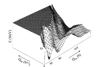
Figure 1: HFB potential energy surface as a function of $\rm q_{20}$ and $\rm q_{30}$ collective variables in ²³⁸U.

For each asymmetry, the determination of scission configurations is made by increasing the elongation step by step: the constrained HFB wave function at a given $q_{20}$ is generated from a previous solution at a slightly lower elongation while keeping $q_{30}$ fixed. This method relies on the scission mechanism studied in Be84 . It is assumed that scission occurs for a given value of $q_{30}$ when the system falls from the so-called ”fission valley” to the ”fusion valley” describing well-separated fragments.

The main criterion used to define exit points and to separate pre- and post- scission configurations is obtained by looking at the nucleon density in the neck: we consider that the system is composed of two fragments when the density in the neck is less than 0.01 nucleon/fm³. This is illustrated in Fig. 2, where density contours are plotted for a given asymmetry $q_{30}$ = 44 $b^{3/2}$ and an increasing elongation. Contour lines are separated by 0.01 nucleon/fm³. Figures 2(a) and 2(b) correspond to pre-scission configurations and figure 2(c) to a post-scission one. Let us note that the two criteria described in Ref. Be84 are also satisfied: a $\simeq$ 15 MeV drop in the energy of the total system, and a $\simeq$ 30$\%$ decrease of the hexadecapole moment are observed when scission occurs.

Figure 2: Proton plus neutron density contours at a given asymmetry $q_{30}$ = 44 b^3/2 for different elongations a) $q_{20}$ = 310 b, b) $q_{20}$ = 320 b and c) $q_{20}$ = 330 b. Contour lines are separated by 0.01 nucleons fm^-3.

It is worth pointing out that the constrained HFB method does not impose an a priori shape to the fissioning system. All types of deformations which are not imposed take the values that minimize the total nuclear energy with both the nuclear mean field and pairing field determined self-consistently. Results concerning fragment deformations at scission will be presented in a forthcoming publication.

Near the exit points, the z-location of the neck, $z_{neck}$, is determined as the z-value for which the nucleon density integrated over $r$ is minimum. Properties of the fragments, such as their masses and their charges, their deformations and the distance between their centers of charge are calculated from integrations in the left and right half-spaces on either sides of the z = $z_{neck}$ plane. As an example, the distance d between the centers of charge of the fragments is plotted in Fig. 3 as a function of the heavy fragment mass. It is found to be maximum for $A_{H}$ = 119 with d = 20.27 fm and minimum for $A_{H}$ = 134 with d = 15.88 fm. Precise values of this fragment center of charge distance are crucial because they govern the Total Kinetic Energy (TKE) distribution, as discussed in Section IV.3. As a test, we have checked that the analytical relations in Eq. (3) are fulfilled.

Figure 3: Distance between the centers of charge of the fragments as a function of the heavy fragment mass.

IV.2 Pairing correlations

Fig. 4 shows the pairing energy $E_{pair}=\frac{1}{2}Tr(\Delta\kappa)$, where $\Delta$ and $\kappa$ are the pairing field and the pairing tensor, respectively. We clearly see that pairing is not constant as a function of elongation. As expected, minima are found inside the wells and maxima at the top of barriers. Furthermore, the total pairing energy, $E_{pair}$, is predicted to be lowest in the asymmetric valley ($E_{pair}\approx$ 6 MeV) and much larger in the symmetric one ($E_{pair}$ $>$ 15MeV). These variations of the pairing correlations are very important since they strongly influence both the collective flux and the occurrence of intrinsic excitations, as is now explained.

Figure 4: Pairing energy as a function of $q_{20}$ along the asymmetric (solid line) and the symmetric (dashed line) fission paths in ²³⁸U.

First, the collective inertia is known to be very sensitive to pairing correlations. The three components $B_{22}$, $B_{33}$ and $B_{23}$ of the inertia tensor in Eq. (12) are plotted in Figs. 5(a), 5(b) and 5(c), respectively, as functions of the elongation along the symmetric (dotted line) and asymmetric (solid line) paths. The two components $B_{22}$ and $B_{33}$ are found to be larger in the symmetric valley than in the asymmetric one (up to a factor of two at large elongation). Furthermore, whereas the non-diagonal inertia component $B_{23}$ is zero for $q_{30}~{}$= 0 by definition, $B_{23}$ is found to be non negligible as soon as the system spreads widely in the asymmetric valley. The coupling brought by $B_{23}$ between the $q_{20}~{}$ and $q_{30}~{}$ modes indicates that, as time evolves, the two collective degrees of freedom exchange energy, which will affect, among other things, the kinetics of the fission process.

Figure 5: Components of the inertia tensor a) $B_{22}$ (in MeV $b^{2}$ $\hbar^{2}$) b) $B_{33}$ (in MeV $b^{3}$ $\hbar^{2}$) c) $B_{23}$ (in MeV $b^{5/2}$ $\hbar^{2}$) as functions of $q_{20}$ along the asymmetric (solid line) and the symmetric (dashed line) fission paths

Second, pairing correlations characterize the amount of superfluidity of the collective flux and the onset of dissipation, in particular between the saddle point and the exit point. In the HFB approach, dissipation requires the creation of two quasiparticle excitations, that is a transfer of energy from the collective motion at least equal to 2$\Delta$, where $\Delta$ is the energy necessary to break a correlated pair. One expects that small values of $\Delta$ will favor ”dissipation”. However, the excitation of the intrinsic structure also depends on the coupling between collective and intrinsic degrees of freedom, which is largely unknown. For this reason, the question of dissipation effects will be addressed in future work. The proton and neutron gaps $2\Delta_{p}$, $2\Delta_{n}$ are plotted in Fig. 6 as functions of elongation along the asymmetric path. The corresponding potential energy curve is also plotted (dotted curve) to guide the eyes. For proton pairing correlations, we find $2\Delta_{p}$ = 2.3 MeV at the top of the second barrier. This value appears to be in good agreement with experimental data Po93 ; Po94 ; Vi00 . As a matter of fact, manifestations of proton pair breaking are observed in ²³⁸U and ²³⁹U nuclei for an excitation energy of 2.3 MeV above the barrier: first the proton odd-even effect observed in the fragment mass distributions decreases exponentially for excitation energy slightly higher than 2.3 MeV Po93 and second, the total kinetic energy drops suddenly  Po94 ; Vi00 .

Figure 6: Twice the proton (solid curve) and neutron (dashed curve) lowest quasi particle energies and potential energy (dotted curve) along the asymmetric path as functions of the elongation in barns.

In Fig. 6 we also see that the proton gap decreases rapidly during the first part of the descent beyond the saddle point, for instance 2$\Delta_{p}$ = 1.4 MeV for $q_{20}$ = 180 b. However, experimental facts show that increasing the excitation energy from 0 to 2.2 MeV above the barrier does not modify the proton odd-even effect. From our point of view, this could be an indication that no proton pairs are broken during the descent from saddle to scission in low energy fission for excitation energies below 2.2 MeV above the barrier. Our interpretation is that the excitation energy supplied during the descent is shared among the collective degrees of freedom and not among intrinsic excitations. This experimental observation gives us some confidence that the neglect of the coupling between collective and intrinsic degrees of freedom is a reasonable approximation to start with in low energy fission.

Finally, no strong odd-even neutron effects are observed for the fragment mass distributions measured in the photofission of ²³⁸U, regardless of excitation energy Po94 . In our calculations the neutron pairing gap is found to be much lower than the proton one, except for 160 $<$ $q_{20}$ $<$ 190 b , as displayed in Fig. 6. At the top of the second barrier the neutron gap is only 2$\Delta_{n}$ = 1.6 MeV. This tends to indicate that neutron pairs are more likely to be broken than proton ones in the even-even ²³⁸U nucleus at low excitation energy. But no definite comparison with experimental data can be made since a precise knowledge of the neutron number of the fission fragments is made extremely difficult by the neutron evaporation. All these remarks concerning pairing correlations a posteriori illustrate the fact that pairing correlations play an essential role and that they should be introduced in dynamical studies of fission.

IV.3 Total Kinetic Energy distribution

As a first estimate, the total kinetic energy $TKE$ of the fragments can be roughly calculated as the Coulomb potential energy $TKE=\frac{Z_{H}Z_{L}e^{2}}{d}$, with d the distance between the centers of charge of the fragments at scission.
Theoretical values calculated along the scission line are shown in Fig. 7 as a function of $A_{H}$, the heavy fragment mass. They are compared to experimental data obtained from the photofission of ²³⁸U using 6.2 MeV bremsstrahlung $\gamma$ rays, corresponding to an excitation energy close to the inner fission barrier height Po94 . We first notice that the general trend of the distribution is rather well reproduced, with a dip at $A_{H}$ = 119 and a peak for $A_{H}$ = 134. Symmetric and asymmetric wings are surprisingly close to experimental data. The agreement indicates that our microscopic approach, together with the prescription explained in Section IV.1 is able to give a realistic description of scission configurations. The main difference with experimental data occurs in the region of the most probable asymmetric fission where the theoretical results overestimate TKE values by $\simeq$ 6$\%$. This discrepancy mainly comes from the fact that the nuclear contribution entering the mutual energy between the two fragments is not strictly zero for the corresponding scission configurations. Furthermore, the – attractive – exchange Coulomb energy between the fragments has been neglected. These two effects could lead to a decrease of TKE values that may reach 10 - 15 MeV.

Figure 7: Total kinetic energy distributions as functions of the heavy fragment mass. Dots indicate experimental data Po94 and the continuous line present predictions.

IV.4 ”One-dimensional” fragment mass distribution

As a first approximation, mass distributions can be derived using the fragmentation model detailed in ref. Li73 . Namely, collective stationary vibrations along the sole mass-asymmetry degree of freedom for nuclear configurations just before scission are studied. The probability of occurrence of a mass asymmetry ($A_{H}$, $A_{L}$) corresponding to a value $q_{30}$ of the octupole moment is then taken as:

$$Y(A_{H},A_{L})=|\Psi_{0}^{+1}(q_{30})|^{2}\ ,$$ (28)

where $\Psi_{0}^{+1}$ is the positive parity eigenstate with lowest energy of the one-dimension collective Hamiltonian $\hat{H^{\prime}}_{coll}$ in the $q_{30}$ variable:

$$\begin{array}[]{lll}\displaystyle\hat{H^{\prime}}_{coll}(q_{30},\frac{\partial}{\partial q_{30}})&=&\displaystyle-\frac{\hbar^{2}}{2}\frac{\partial}{\partial q_{30}}\frac{1}{\mathcal{M}_{3}(q_{30})}\frac{\partial}{\partial q_{30}}\\ &&\\ &&\displaystyle+V(q_{30})-\Delta V_{3}(q_{30})\ .\end{array}$$ (29)

Here, $V(q_{30})$ is the HFB deformation energy along the scission line $q_{20}$ = $q_{20}^{s}$ = $f(q_{30})$, $\mathcal{M}_{3}(q_{30})$ is the collective inertia, and $\Delta V_{3}(q_{30})$ the zero-point-energy correction (ZPE). The Hamiltonian of Eq. (29) is derived from the usual GOA reduction of the one-dimensional Hill-Wheeler stationary equation obtained by taking for the generator coordinate the curvilinear abscissa $s(q_{20},q_{30})$ along the scission line. A change of variable is then performed in order to express all quantities as functions of $q_{30}$. It is easy to show that the inertia and ZPE correction appearing in Eq. (29) are related to those entering the full two-dimensional Hamiltonian (12):

$$\mathcal{M}_{3}(q_{30})=(\frac{df}{dq_{30}})^{2}\,M_{22}+2(\frac{df}{dq_{30}})\,M_{23}+M_{33},$$ (30)

$$\Delta V_{3}(q_{30})=\frac{\mathcal{G}_{3}(q_{30})}{2\mathcal{M}_{3}(q_{30})},$$ (31)

with

$$\mathcal{G}_{3}(q_{30})=(\frac{df}{dq_{30}})^{2}\,G_{22}+2(\frac{df}{dq_{30}})\,G_{23}+G_{33},$$ (32)

where $M_{ij}$ are the inertia defined in Eq. (13) and $G_{ij}$ the components of the overlap tensor calculated in the cranking approximation using the moments of Eq. (14).

Clearly, the model based on the Hamiltonian (29) amounts to ignore all the effects of the dynamics along the elongation degree of freedom from the first well to scission. We call the mass distribution obtained in this way a ”one-dimensional” mass distribution.

The HFB potential energy $V(q_{30})$ calculated along the scission line is plotted in Fig. 8 as a function of the octupole moment. The lowest energy is obtained for $q_{30}$ = $\pm$ 44 b, corresponding to the most probable fission. A secondary minimum is found for $q_{30}$ = 0 b. These two wells are separated by a 11 MeV high barrier.

Figure 8: Potential energy along the scission line as a function of the octupole moment.

”One-dimensional” distributions are shown in Fig. 9 where the mass yield Eq. (28) is plotted (solid line) together with the Wahl evaluation (dashed line) for 46 keV neutron induced fission on ²³⁷U Wa02 . The maxima of the theoretical curve occur at $A_{H}$ = 134, $A_{L}$ = 94 values corresponding to the minima of the potential energy along the scission line. The fact that the experimental curve maxima lie close to these values indicate that the most probable fragmentation is due essentially to the properties of the potential energy surface at scission, i.e mainly to shell effects in the nascent fragments. However, the ”one-dimensional” approach does not reproduce neither the experimental peak-to-valley ratio nor the experimental widths of the distributions - the theoretical widths are twice smaller than the Wahl evaluated ones-.

Figure 9: Comparison between the ”one-dimensional” mass fragment distribution obtained from (28) (solid line), and the Wahl evaluation (dashed line) Wa02 .

One must note however that only the solution of Eq. (29) with lowest energy $\Psi_{0}^{+1}$ has so far been considered. This is certainly an oversimplifying assumption since, the wave function describing the collective evolution of the nucleus will undoubtedly possess a more complicated structure at the time of reaching the scission line. In particular, as mentioned in ref. Ma74 , $n>0$ states $\Psi_{n}^{\pi}$, solutions of Eq. (29), may become excited due to the interaction between $q_{20}$ and $q_{30}$ degrees of freedom. Let us mention that, in Ref Ma74 the population of the eigenstates has been assumed to follow a Boltzmann law governed by a temperature parameter. In Ref. Ma76 , the elongation degree of freedom has been introduced using a classical approximation.

Amplitudes of the first six collective states $\Psi_{n}^{\pi}$, n = 0 … 5, solutions of Eq. (29) are displayed in Fig. 10 as functions of the fragment mass. As is well-known, such $\Psi_{n}^{\pi}$ states are eigenstates of the parity operator $\Pi$ with eigenvalues ${\pi}$. Positive and negative parity states are plotted in solid and dotted lines, respectively. Each pair of $\pi$ = +1 and $\pi$ = -1 levels is degenerate in energy because the potential is symmetric with respect to the $q_{30}$ $\rightarrow$ -$q_{30}$ transformation, and because the barrier between the two asymmetric wells is high (11 MeV) (see Fig. 8). We observe in Fig. 10 that the excited states are more spread over mass than the ground state. For example, the wave functions $\Psi_{4}^{+1}$ and $\Psi_{5}^{-1}$ displayed in Fig. 10c) display non-zero values up to $A_{H}\approx$ 156 whereas the lowest energy wave functions $\Psi_{0}^{+1}$ and $\Psi_{1}^{-1}$ in Fig. 10a) are localized in the domain 132 $<$ $A_{H}$ $<$ 144. Therefore, we can expect that the introduction of these excited states in the definition of the mass yield Eq. (28) will broaden the mass distribution in the asymmetric region.

Figure 10: Amplitudes of the first six collective states in the asymmetry variable at scission as functions of the fragment mass. Positive (negative) parity states are plotted in solid (dotted) lines. Excitation energies, measured from the lowest energy state, are a) E = 0 MeV, b) E = 3.09 MeV and, c) E = 4.76 MeV.

V Dynamical results

V.1 Initial states

The time-dependent evolution of the system has been calculated using different initial conditions in the first well of the potential energy surface. Calculations have been performed from t = 0 up to maximum times for which the flux of the time-dependent collective wave function along the scission line has become stabilized.

We first discuss the effect of the structure of the initial state on the mass distribution. In order to define the initial conditions we imagine that the nucleus is a compound system described in terms of complicated quasi-stationnary states which decay into various channels (neutron and $\gamma$-ray emission and fission). In the case of the even-even K = 0 ²³⁸U nucleus studied here, we assume that states which decay through fission can be described by the simple form:

$${|{\Psi_{P,K=0,I,M}}\rangle}=(2\pi)^{-\frac{1}{2}}Y_{I,M}(\Omega)\;\int dq\;f_{n}^{\pi}(q,t=0)\;{|{\phi(q)}\rangle},$$ (33)

where $Y^{M}_{I}(\Omega)$ are spherical harmonics and $\Omega$ the Euler angles relating the intrinsic axes of the nucleus to the laboratory frame of reference.

The parity quantum number P is related to the intrinsic parity $\pi$ by the following relation :

$$P=\pi(-1)^{I},$$ (34)

where I is the spin of the fissioning system. In Eq. (33), q is the set of all relevant nuclear collective deformations which, in the present work (see Eq. (8)) is restricted to $(q_{20},q_{30})$.
As already mentioned in Section II, initial states $g_{n}^{\pi}(q_{20},q_{30},t=0)$ (related to the $f_{n}^{\pi}(q_{20},q_{30},t=0)$ functions as in Eq. (11)) are taken as eigenstates of the modified two-dimensional first well $V^{\prime}(q_{20},q_{30})$, where the potential has been extrapolated at large deformations as shown in Fig. 11. They are solutions of the equation:

$$\hat{H^{\prime}}_{coll}\;g_{n}^{\pi}(q_{20},q_{30},t=0)=E^{\pi}_{n}\;g_{n}^{\pi}(q_{20},q_{30},t=0)\ ,$$ (35)

where $\hat{H^{\prime}}_{coll}$ is the Hamiltonian defined in Eq. (12) with $V(q_{20},q_{30})$ replaced by $V^{\prime}(q_{20},q_{30})$.

Because $H^{\prime}_{coll}(q_{20},q_{30},\frac{\partial}{\partial q_{20}},\frac{\partial}{\partial q_{30}})$ = $H^{\prime}_{coll}(q_{20},-q_{30},\frac{\partial}{\partial q_{20}},-\frac{\partial}{\partial q_{30}})$ these initial states can be chosen as eigenstates of the parity operator with eigenvalues $\pi$ = $\pm$ 1 Me95 :

$$g_{n}^{\pi}(q_{20},-q_{30},t=0)=\pi\;g_{n}^{\pi}(q_{20},q_{30},t=0)\ .$$ (36)

The potential curves $V(q_{20},q_{30}=0)$ and $V^{\prime}(q_{20},q_{30}=0)$ including zero-point-energy corrections are displayed in Fig. 11. The eigen-energies of $H^{\prime}_{coll}$ are also shown. Excitation energies of the compound nucleus in the interval $[$ $B_{I}$ , $B_{I}$ +2.5 MeV $]$ will be considered in this work focussing on low-energy fission, where $B_{I}$ is the first barrier height. In this energy range, the mean-level spacing is found to be around 130 keV. Therefore, 19 states are possible initial candidates for our dynamical calculations. All these states are located above the outer symmetric saddle point but below the outer asymmetric one. They correspond to multi- quadrupole and octupole phonons, and have different components along the $q_{30}$ and $q_{20}$ directions. Significant effects on the fragment mass distributions are mainly due to the parity of the initial states.

Figure 11: Potential curves $V(q_{20},q_{30}=0)$ and $V^{\prime}(q_{20},q_{30}=0)$ including zero-point-energy corrections (continuous and dotted lines, respectively), and collective eigenstates of the modified $V^{\prime}(q_{20},q_{30}=0)$ potential (horizontal segments).

In Fig. 12, fragment mass distributions, calculated with formula (25) and initial states of definite parity, are plotted separately. The solid and dotted curves correspond to initial states whose intrinsic parity is positive or negative exclusively. They are located at 2.4 MeV and 2.3 MeV above the first barrier, respectively.

Figure 12: Fragment mass distributions obtained for initial states having positive parity (solid line) and negative parity (dotted line).

We see that the main difference between the two results is the peak-to-valley ratio which is of the order of 50 for the positive parity initial state and infinite for the negative one. The fact that no symmetric fission is found when the initial state has a negative parity is due to the fact that $g_{n}^{-1}(q_{20},q_{30}=0,t)$ = 0 if $\pi$ = -1 for any time t. As a consequence, the flux of the wave function through the scission line at $q_{30}$ = 0 vanishes.
In the applications presented below we use initial states that don’t have a definite parity. As we observed at the end of section III there are interferences between states of different parities in the calculation of the flux. However, due to the symmetries of the inertia tensor, these interferences do not contribute to the symmetric mass fragmentation. ¿From the previous discussion we infer that our predictions of symmetric fission will be affected by the proportions of collective states with negative and postive intrinsic parity. In order to get an estimate of these proportions we assume that they are the same as in the compound sytem n+²³⁷U. More precisely, by using Eq. (34) we define fission cross sections, $\sigma$($\pi$ = +1,E) and $\sigma$($\pi$ = -1,E) corresponding to components of intrinsic parity in the compound system through the relations:

$$\begin{array}[]{lll}\sigma(\pi=-1,E)&=\displaystyle\sum_{I=2p,P=-1}&\sigma_{CN}(P,I,E)\;P_{f}(P,I,E)\\ &\displaystyle+\sum_{I=2p+1,P=+1}&\sigma_{CN}(P,I,E)\;P_{f}(P,I,E)\ ,\\ &&\\ \sigma(\pi=+1,E)&=\displaystyle\sum_{I=2p,P=+1}&\sigma_{CN}(P,I,E)\;P_{f}(P,I,E)\\ &\displaystyle+\sum_{I=2p+1,P=-1}&\sigma_{CN}(P,I,E)\;P_{f}(P,I,E)\ ,\end{array}$$ (37)

where E, P, $\sigma_{CN}(P,I,E)$ and $P_{f}(P,I,E)$ are the energy, the parity (defined in Eq. (34)), the formation cross section and the fission probability of the compound nucleus, respectively.

Formation cross sections have been calculated using the Hauser-Feschbach theory with the optical potential model of Ref. optic and fission probabilities have been deduced from a statistical model calculation WKB .

Then, we define probabilities by the following fractions:

$$\begin{array}[]{lll}p^{-}(E)&=&\displaystyle\frac{\sigma(\pi=-1,E)}{\sigma(\pi=-1,E)+\sigma(\pi=+1,E)}\ ,\\ &&\\ p^{+}(E)&=&\displaystyle\frac{\sigma(\pi=+1,E)}{\sigma(\pi=-1,E)+\sigma(\pi=+1,E)}\ .\end{array}$$ (38)

They represent the population of states in the compound system which have a given intrinsic parity and which decay to fission. It is with the help of these probabilities that we determine the mixing of parities in the initial states. Numerical values for the reaction n+²³⁷U are given in Table 1 for two excitation energies as measured from the top of the first barrier.

E (MeV)	1.1	2.4
$p^{+}(E)$ $\%$	77	54
$p^{-}(E)$ $\%$	23	46

Table 1: Percentages of positive and negative intrinsic parity states populated in the compound nucleus ²³⁸U by the n+²³⁷U reaction for two excitation energies.

Mass distributions obtained for these two energies are displayed in Fig. 13: the solid and dashed lines correspond to the two energies, 2.4 MeV and 1.1 MeV respectively.

Figure 13: Fragment mass distributions obtained for two initial states. Solid line: E = 2.4 MeV with $p^{+}$ =54 $\%$ and $p^{-}$ =46 $\%$. Dashed line: E = 1.1 MeV with $p^{+}$ = 77 $\%$ and $p^{-}$ = 23 $\%$.

One observes that the symmetric fragmentation is slightly higher at excitation energy 1.1 MeV than at 2.4 MeV. Clearly, this approach does not reproduce an essential feature of measured or evaluated mass fragment distributions namely, a sensitive increase of the symmetric fission yield with increasing neutron energy. As can be inferred from previous discussions, this discrepancy is a direct consequence of the rapid decrease with increasing energy of positive parity components in the initial state. More detailed comparisons of the theoretical predictions with Wahl evaluations Wa02 Fig. 14 indicate, however, that the microscopic approach reproduces successfully various characteristics of the mass distribution.

Figure 14: Theoretical mass distributions (solid lines) are compared with the Wahl evaluations of neutron induced fission of ²³⁸U Wa02 (dashed lines). Excitation energies of the compound ²³⁸U nucleus measured above the barrier are a) E = 2.4 MeV, b) E = 1.1 MeV

For instance, the comparison at 2.4 MeV shows that the main features of Wahl’s distribution, position and height of the maxima, ratio peak to valley and broadening of the distribution as well, are satisfactorily reproduced by the theory. The agreement at lower energy is not as good, due essentially to the discrepancy mentioned above.

Initial conditions appear to be crucial for the prediction of mass distributions at low energy. In view of the quality of the results presented above we consider studying more carefully this question in future works.

V.2 Dynamical effects

In order to analyze the influence of dynamical effects, the fragment mass distribution obtained for the initial state located 2.4 MeV above the first barrier shown in Fig. 14a) is compared in Fig. 15 with our previous ”one-dimensional” distribution. Fig. 15 also shows the evaluated data from the Wahl systematics (dashed curve) Wa02 .

Figure 15: Comparison between the ”one-dimensional” mass distribution of Fig. 9 (dotted line), the mass distribution resulting from the dynamical calculation (solid line) with the initial state state located 2.4 MeV above the barrier, and the Wahl evaluation (dashed line) Wa02 .

We first note that the maxima of the two theoretical distributions are both located around $A_{H}$ = 134 and $A_{L}$ = 104, in good agreement with evaluated data. As already mentioned in Section IV.4, this is a confirmation that the most probable fragmentation is due essentially to shell effects in the nascent fragments and not to dynamical effects. The widths of the peaks obtained from the full dynamical calculation are much larger- about twice as large - than those of the ”one-dimensional” one, and consequently they are in much better agreement with the Wahl evaluated data. Clearly the dynamics is found to play a major role in the broadening of the fragment mass distributions. In the present dynamical calculation the broadening is clearly due to the interaction between the elongation and the asymmetry degrees of freedom, which results from both the potential energy and the inertia variations. As already discussed in Section III, these effects are especially important in the descent from saddle to scission, where the inertia component $B_{23}$ is found to be large (see Fig. 5). In fact the cross term in the kinetic energy of the collective Hamiltonian appears to be responsible for exchanges of energy between the two modes and for the spreading of the time-dependent wave function in the asymmetric valley.
In order to quantitatively analyze those effects, the time dependent wave function $g(q_{20},q_{30},t)$ has been expanded over the ”one-dimensional” states $\Psi_{n}^{\pi}(q_{30})$ described in Section IV.4 along the line $q_{20}$ = $(q_{20})_{s}$ = $f(q_{30})$:

$$g((q_{20})_{s},q_{30},t)=\sum_{n}C_{n}(t)\;\Psi_{n}^{\pi}(q_{30}).$$ (39)

The weight coefficients $C_{n}(t)$ can be calculated as:

$$C_{n}(t)=\int\;dq_{30}\;g((q_{20})_{s},q_{30},t)\;\Psi_{n}^{\pi}(q_{30}),$$ (40)

and the fraction of each ”one-dimensional” state contained in the dynamical solution at scission is given by:

$$R_{n}(t)=\displaystyle\frac{|C_{n}(t)|^{2}}{\sum_{m}|C_{m}(t)|^{2}}.$$ (41)

Results for $R_{n}$(t = 0.96 $10^{-20}$ s) are listed in table 2 in the case of the dynamical wave function corresponding to the initial state considered here.

n	1-2	3-4	5-6	7-8	9-10
$R_{n}$ $\%$	35.2	8.6	36.7	6.9	12.6

Table 2: Percentages of the ”one-dimensional” states contained in the dynamical solution at scission for t = 0.96 $10^{-20}$ s.

These results indicate that the dynamical wave function is spread over many ”one-dimensional” states $\Psi_{n}^{\pi}$ and that the relative contribution of the two low-energy states is only 35.2 $\%$. As it appears, the ”one-dimensional” definition (28) of the fragment yield is not pertinent, and dynamical effects should be fully taken into account in order to obtain realistic predictions for fragment mass distributions.

VI Conclusion

In this work, we have presented a theoretical framework and numerical techniques allowing one to describe fission mass distribution in a completely microscopic way. The method is based on a HFB description of the internal structure of the fissioning system. The collective dynamics is derived from a time-dependent quantum-mechanical formalism where the wave-function of the system is of GCM form. A reduction of the GCM equation to a Schrödinger equation is made by means of usual techniques based on the Gaussian Overlap Approximation. Such an approach has the advantage of describing the evolution of heavy nuclei toward fission in a completely quantum-mechanical fashion and without phenomenological parameters.
Properties of the fissioning system which have a large influence on collective dynamics have been discussed. Among them, the most important is the variation with deformation of the nuclear superfluidity induced by pairing correlations. In addition to strongly influence the magnitude of the collective inertia, these correlations are essential in our approach because they validate the adiabatic hypothesis as a first approximation for the description of low energy fission.
In the present application of this method to ²³⁸U fission, two kinds of observables have been examined and compared to experimental data: the kinetic energy distribution and mass distribution of fission fragments. The kinetic energy distribution, which has been derived from the mutual Coulomb energy of the fragments at scission, is found to be in good agreement with data. A small discrepancy (6$\%$) is found around the most probable fragmentation region, which could originate from the fact that the nuclear contribution entering the mutual energy between the two fragments is not strictly zero for the corresponding scission configurations and that the attractive exchange Coulomb energy between the fragments has been neglected. Concerning fragment mass distributions, the main result of the present study is that dynamical effects taking place all along the evolution of the nucleus are essential in order to obtain widths in agreement with experimental data. In contrast, the maxima of the distributions are determined by the static properties of the potential energy surface in the scission region, that is by shell effects in the nascent fragments. Finally, the influence of the choice of the initial state has been studied. In particular, symmetric fragment yields are found to be strongly influenced by the parity composition of the initial state. The quality of the results reported here encourages us to pursue further studies of fission along these lines, with some additional improvements. For instance, as suggested by the work cited in Ref. Mo04 , we cannot exclude that several valleys due to other collective modes, such as hexadecapole or higher multipole deformation, can appear in some fissioning systems. Extensions to microscopic calculations involving three or more collective coordinates are envisaged.

VII Acknowledgment

We would like to thank D. Bouche, N. Carjan and A. Rizea for useful advice concerning numerical methods and Professors F. Goennenwein and K.-H. Schmidt for enlightening discussions on experimental results. Finally, the authors wish to express their gratitude to Professor F. Dietrich and W. Younes for valuable discussions, and for a critical review of the manuscript.

Appendix A Hamiltonian matrix

Starting from the functional Eq. (15), the matrix elements of the Hamiltonian matrix K can be expressed from:

$$\left(\hat{H}_{coll}g\right)(i,k,t)=\displaystyle\sum_{jl}K_{ik,jl}\;g(j,l,t).$$ (42)

By writing:

$$\hat{H}_{coll}=\sum_{i,j=2}^{3}\hat{T}_{ij}+\tilde{V}(q_{20},q_{30})\ ,$$ (43)

with

$$\begin{array}[]{rll}\displaystyle\hat{T}_{ij}&=&\displaystyle-\frac{\hbar^{2}}{2}\frac{\partial}{\partial q_{i0}}B_{ij}(q_{20},q_{30})\frac{\partial}{\partial q_{j0}}\ ,\\ \displaystyle\tilde{V}(q_{20},q_{30})&=&\displaystyle V(q_{20},q_{30})-\sum_{i,j=2}^{3}\Delta V_{i,j}(q_{20},q_{30})\ ,\end{array}$$ (44)

the different terms contributing to Eq. (42) are:

$$\begin{array}[]{ll}\displaystyle(\hat{T}_{22}+\hat{T}_{33})g(i,k,t)&=\displaystyle\frac{1}{4\Delta q_{20}^{2}}\{[-B_{22}(i-1,k)-B_{22}(i,k)]g(i-1,k,t)\\ &\displaystyle+[B_{22}(i-1,k)+2B_{22}(i,k)+B_{22}(i+1,k)]g(i,k,t)\\ &\displaystyle+[-B_{22}(i,k)-B_{22}(i+1,k)]g(i+1,k,t)\}\\ &\displaystyle+\frac{1}{4\Delta q_{30}^{2}}\{[-B_{33}(i,k-1)-B_{33}(i,k)]g(i,k-1,t)\\ &\displaystyle+[B_{33}(i,k-1)+2B_{33}(i,k)+B_{33}(i,k+1)]g(i,k,t)\\ &\displaystyle+[-B_{33}(i,k)-B_{33}(i,k+1)]g(i,k+1,t)\}\ ,\end{array}$$ (45)

$$\begin{array}[]{ll}\displaystyle(\hat{T}_{23}+\hat{T}_{32})g(i,k,t)&=\displaystyle\frac{1}{16\Delta q_{20}\Delta q_{30}}\{[B_{23}(i-1,k+1)+B_{23}(i,k+1)\\ &\displaystyle+B_{23}(i-1,k)+B_{23}(i,k)]g(i-1,k+1,t)\\ &\displaystyle+[B_{23}(i-1,k-1)+B_{23}(i+1,k+1)\\ &\displaystyle-B_{23}(i-1,k+1)-B_{23}(i+1,k-1)]g(i,k,t)\\ &\displaystyle+[-B_{23}(i-1,k)-B_{23}(i,k)\\ &\displaystyle-B_{23}(i-1,k-1)-B_{23}(i,k-1)]g(i-1,k-1,t)\\ &\displaystyle+[-B_{23}(i,k+1)-B_{23}(i+1,k+1)\\ &\displaystyle-B_{23}(i,k)-B_{23}(i+1,k)]g(i+1,k+1,t)\\ &\displaystyle+[B_{23}(i,k)+B_{23}(i+1,k)\\ &\displaystyle+B_{23}(i,k-1)+B_{23}(i+1,k-1)]g(i+1,k-1,t)\},\end{array}$$ (46)

and

$$\tilde{V}(i,k)\;g(i,k,t)=\{V(i,k)\;-\Delta V_{22}(i,k)-\Delta V_{22}(i,k)-2\Delta V_{23}(i,k)\}g(i,k,t).$$ (47)

The labels $i$ and $k$ are related to $q_{20}$ and $q_{30}$, respectively, and $\Delta q_{20}$ and $\Delta q_{30}$ are the associated discretization steps. The following approximation has been used for the inertia term:

$$B_{jj}(i\pm\frac{1}{2},k)\approx\frac{1}{2}(B_{jj}(i,k)+B_{jj}(i\pm 1,k))\ ,$$ (48)

and, for products $F$ of two functions $F_{1}$ and $F_{2}$ the following prescription has been assumed:

$$\begin{array}[]{ll}\displaystyle F(i+\frac{1}{2},k)&=\displaystyle F_{1}(i+\frac{1}{2},k)F_{2}(i+\frac{1}{2},k)\\ &\displaystyle\approx\frac{1}{4}(F_{1}(i+1,k)+F_{1}(i,k))(F_{2}(i+1,k)+F_{2}(i,k))\ .\end{array}$$ (49)

References

- (1) M Bernas, P. Armbruster, J. Benlliure, A. Boudard, E. Casarejos, S. Czajkowski, T. Enqvist, R. Legrain, S. Leray, B. Mustapha, P. Napolitani, J. Pereira, F. Rejmund, M.-V. Ricciardi, K.-H. Schmidt, C.Stephan, J. Taieb, L. Tassan-Got and C. Volant, Nucl. Phys. A725 (2003) 213
- (2) K. H. Schmidt, S. Steinhauser, C. Bockstiegel, A. Heinz, A.R. Junghans, J. Benlliure, H.-G. Clerc, M. de Jong, J. Muller, M.Pfutzner and B. Voss, Nucl. Phys. A665 (2000) 221
- (3) J. Benlliure, A.R. Junghans and K.H. Schmidt, Eur. Phys. J. A13 (2002) 93
- (4) P. Möller, D.G. Madland, A.J. Sierk and A. Iwamoto, Nature 409 (2001) 785
- (5) V V. Pashkevich, Nucl. Phys. A477 (1988) 1
- (6) B. D. Wilkins, E. P. Steinberg, and R. R. Chasman, Phys. Rev. C14 (1976) 1832
- (7) U. Brosa, Phys. Rev. C38 (1988) 1944
- (8) A. V. Karpov, P. N. Nadtochy, D. V. Vanin and G. D. Adeev, Phys. Rev. C63 (2001) 054610
- (9) J. W. Negele, S. E. Koonin, P. Möller, J. R. Nix and A. J. Sierk, Phys. Rev. C17 (1978) 1098
- (10) J.-F. Berger, M. Girod and D. Gogny, Nucl. Phys. A428 (1984) 23c
- (11) J. Moreau and K. Heyde in ”The nuclear fission process” C. Wagemans CRC Press (1991) 238
- (12) J. Decharge and D. Gogny, Phys. Rev. C21 (1980) 1568
- (13) J-F. Berger M. Girod and D. Gogny, Comp. Phys. Comm. 63 (1991) 365
- (14) P. Ring and P. Schuck, The Nuclear Many Body Problem, Springer-Verlag New-York, USA (1980)
- (15) L.M. Robledo, J.L. Egido, B. Nerlo-Pomorska and K. Pomorski PL B201 (1988) 409
- (16) J. Libert, M. Girod and J.-P. Delaroche, Phys. Rev. C60 (1999) 054301
- (17) W. H. Press, B. P. Flannery, S. A. Teukolsky,and W. T. Vetterling, in Numerical recipes: the art of scientific computing, (Cambridge University Press, Cambridge, 1986)
- (18) N. Carjan, M. Rizea and D. Strottman, Rom. J. Phys. 47 (2002) 221
- (19) O. Serot, N. Carjan and D. Strottman, Nucl. Phys. A569 (1994) 562
- (20) S. Pomme, E. Jacobs, K. Persyn, D. De Frenne, K. Govaert, and M.-L. Yoneama, Nucl. Phys. A560 (1993) 689
- (21) S. Pomme, E. Jacobs, M. Piessens, D. De Frenne, K. Persyn, K. Govaert, and M.-L. Yoneama, Nucl. Phys. A572 (1994) 237
- (22) F. Vives, F.-J. Hambsch, H. Bax and S. Oberstedt, Nucl. Phys. A662 (2000) 63
- (23) P. Lichtner, D. Drechsel, J. Maruhn and W. Greiner, Phys. Lett. B45 (1973) 175
- (24) A. C. Wahl, Systematics of fission-product yields, bf LA-13928, Los Alamos National Laboratory, (2002)
- (25) J. Maruhn and W. Greiner, Phys. Rev. Lett. 32 (1974) 548
- (26) J. A. Maruhn and W. Greiner, Phys. Rev. C13 (1976) 2404
- (27) J. Meyer, P. Bonche, M.S. Weiss, J. Dobaczewski, H. Flocard and P.-H. Heenen, Nucl. Phys. A588 (1995) 597
- (28) W.Younes and H.C. Britt, Phys.Rev. C67 (2003) 024610
- (29) W. Younes, private communication
- (30) P. Möller, A. J. Sierk, and A. Iwamoto, Phys. Rev. Let. 92 (2004) 072501