chiral symmetry
and
parametrization of scalar resonances

Abstract

The linear $\sigma$-model is used to study the effects of chiral symmetry in unitarized amplitudes incorporating scalar resonances. When just a single resonance is present, we show that the iteration of a chiral tree amplitude by means of regularized two-pion loops preserves the smallness of $\pi\pi$ interaction at low energies and estimate the importance of pion off-shell contributions. The inclusion of a second resonance is performed by means of a chiral extension of the linear $\sigma$-model lagrangian. The new $\pi\pi$ ampitude at tree level complies with low-energy theorems, depends on a mixing angle and has a zero for a given energy between the resonance masses. The unitarization of this amplitude by means of two-pion loops preserves both its chiral low energy behavior and the position of this zero confirming, in a lagrangian framework, conclusions drawn previously by Törnqvist. Finally, we approximate and generalize our results and give a friendly expression that can be used in the parametrization of $N$ coupled scalar resonances.

I introduction

Scalar mesons have since long proved to be the most elusive states in low energy hadron physics. At present, after decades of research, one still is not sure as how to classify them into multiplets or what their quark and gluon contents areCl . On the empirical side, one also finds important uncertainties in masses, widths, or even in the very existence of some states.

Part of the difficulties in understanding the scalar sector may be ascribed to the fact that resonances can couple through intermediate states containing two identical pseudoscalar particles. About ten years ago this important aspect of the problem was discussed by TörnqvistTor , who set a rather useful and comprehensive theoretical framework for describing the role of such couplings, based on the unitarized quark model. The interference of resonances was also considered by SvecSv , using phase shifts and non-relativistic quantum mechanics.

The interest in the scalar sector was revived recently by evidences provided by the E791 Fermilab experiment of the existence of resonances with low masses and large widths in the decays $D^{+}\rightarrow(\pi^{-}\pi^{+})\;\pi^{+}$cbpfD1 and $D_{s}^{+}\rightarrow(K^{-}\pi^{+})\;\pi^{+}$cbpfD2 . The former finding was confirmed in a number of other reactions: $D^{0}\rightarrow K_{s}^{0}\;(\pi^{-}\pi^{+})$Cleo ; Belle ; BaBar1 , $\phi\rightarrow\gamma\;(\pi^{-}\pi^{+})$Kloe , $J/\psi\rightarrow\omega\;(\pi^{-}\pi^{+})$Bes , $B^{+}\rightarrow(\pi^{-}\pi^{+})\pi^{+}$BaBar2 . These recent results motivate the present work, in which we discuss how chiral symmetry affects the low-energy region of these processes and may influence the parameters of a light and broad resonance and its couplings to heavier partners.

Quantum chromodynamics (QCD) is the basic theoretical framework for the study of hadronic processes, but its non-Abelian structure hampers analytic low-energy calculations. Therefore one needs to resort to effective theories, which mimic QCD. In order to be really effective, these theories must be Poincaré invariant and possess approximate either $SU(2)\times SU(2)$ or $SU(3)\times SU(3)$ symmetries, broken by small Goldstone boson masses. For the sake of simplicity, we restrict ourselves to the $SU(2)$ sector.

The unitarized elastic $\pi\pi$ amplitudes discussed here are obtained by iterating their tree counterparts. In section 2, we review the main features of the $\sigma$-model description of these building blocks and, in section 3, derive a unitarized amplitude for the single resonance case. As a large part of the algebraic effort needed in this result is associated with the treatment of pion-off shell effects, in section 4 we assess their numerical importance. In section 5 we extend the linear $\sigma$-model in order to allow the inclusion of a second resonance and, in section 6, study its coupling to the first one by means of two-pion loops. Finally, in section 7, we summarize our results and give a simple expression that can be applied in data analyses. We have tried to make it as self contained as possible, so that it could be read directly by those people not interested in technical details.

II chiral symmetry

The intense activity on chiral perturbation theory performed in the last twenty years has made clear the convenience of working with non-linear realizations of the symmetry. On the other hand, when dealing with scalar resonances, one may be tempted to employ the old and well known linear $\sigma-$model. The advantage of the former is that it is more general and incorporates all the possible freedom compatible with the symmetry. On the other hand, it is non-renormalizable and one has to resort to order-by-order renormalization in order to circumvent this difficulty. The less general linear model is not affected by this problem. As we discuss in the sequence, for a given choice of parameters, results from the linear and non-linear models become identical at tree level.

In the framework of chiral symmetry, the inclusion of resonances must be performed in such a way as to preserve the low-energy theorems for $\pi\pi$, scattering derived by means of current algebra. Quite generally, the amplitude $T_{\pi\pi}$ for the process $\pi^{a}(p)\,\pi^{b}(q)\rightarrow\pi^{c}(p^{\prime})\,\pi^{d}(q^{\prime})$ can be written as

$$T_{\pi\pi}=\delta_{ab}\delta_{cd}\,A(s)+\delta_{ac}\delta_{bd}\,A(t)+\delta_{ad}\delta_{bc}\,A(u)\;,$$ (1)

with $s=(p\!+\!q)^{2}$, $t=(p\!-\!p^{\prime})^{2}$, $u=(p\!-\!q^{\prime})^{2}$. A low-energy theorem ensures that the functions $A(x)$, for $x=s,t,u$, must have the form

$$A(x)=\frac{x-\mu^{2}}{f_{\pi}^{2}}+\cdots\;,$$ (2)

where $\mu$ and $f_{\pi}$ are the pion mass and decay constant and the ellipsis indicates higher order contributions.

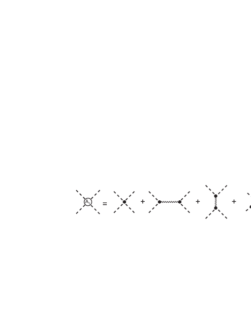
Figure 1: Tree amplitude $A_{t}$; dashed and thin wavy lines represent pions and a scalar resonance.

When a scalar-isoscalar resonance is present, the tree level amplitude for $\pi\pi$ scattering is given by the four diagrams of fig.1, irrespectively of whether the symmetry is implemented linearly or not. We begin by considering the linear $\sigma-$model, described by the lagrangian

$${\cal{L}}_{\sigma}=\frac{1}{2}\left(\partial_{\mu}\sigma\;\partial^{\mu}\sigma+\partial_{\mu}\mbox{\boldmath$\pi$}\!\cdot\!\partial^{\mu}\mbox{\boldmath$\pi$}\right)-\frac{m^{2}}{2}\left(\sigma^{2}\!+\!\mbox{\boldmath$\pi$}^{2}\right)-\frac{\lambda}{4}\left(\sigma^{2}\!+\!\mbox{\boldmath$\pi$}^{2}\right)^{2}+c\,\sigma\;.$$ (3)

Denoting by $f$ the fluctuations of the scalar field and using $\sigma=f_{\pi}\!+\!f$, one finds, at tree level,

$$\mu^{2}=m^{2}+\lambda f_{\pi}^{2}\;,\;\;\;\;\;\;c=\mu^{2}f_{\pi}\;,\;\;\;\;\;\;M_{\sigma}^{2}=2\lambda f_{\pi}^{2}+\mu^{2}\;,$$ (4)

$M_{\sigma}$ being the $\sigma$ mass. The $\pi\pi$ scattering amplitude is

$$A_{t}(x)=-2\;\lambda-\;\frac{4\;\lambda^{2}\;f_{\pi}^{2}}{x-M_{\sigma}^{2}}\;,$$ (5)

where the subscript $t$ stands for tree and the two contributions on the r.h.s. arise respectively from the four-pion vertex and one of the resonance terms in fig.1. Comparing this result with eq.(2), one learns that none of these contributions is isolatedly compatible with the low-energy theorem. However, when both terms are added, one has

$$A_{t}(x)=\frac{x\!-\!\mu^{2}}{f_{\pi}^{2}}\;\left[1-\;\frac{x\!-\!\mu^{2}}{x\!-\!M_{\sigma}^{2}}\right]\;,$$ (6)

and consistency becomes explicit, since $M_{\sigma}^{2}>>\mu^{2}\sim x$. This result conveys an important message, namely that, in the linear model, the resonance and the non-resonating background must always be treated in the same footing, for the sake of preserving chiral symmetry. As we discuss in the sequence, this issue is especially relevant for the definition of the resonance width.

In the alternative approach, the scalar field $f$ couples to pion fields $\phi$, which behave non-linearly under chiral transformationsWei . In this new framework, the field $f$ is assumed to be a true chiral scalar, invariant under both vector and axial transformations, and should not be confused with $\sigma$, the chiral partner of the pion in the linear $\sigma$-model. The effective lagrangian for this system is written asMR

$${\cal{L}} = \frac{1}{2}\left(\partial_{\mu}f\;\partial^{\mu}f-M_{\sigma}^{2}f^{2}\right)+\frac{1}{2f_{\pi}}\left(f_{\pi}+c_{\chi}f\right)\left(\partial_{\mu}\mbox{\boldmath$\phi$}\!\cdot\!\partial^{\mu}\mbox{\boldmath$\phi$}+\partial_{\mu}\sqrt{f_{\pi}^{2}-\mbox{\boldmath$\phi$}^{2}}\;\partial^{\mu}\sqrt{f_{\pi}^{2}-\mbox{\boldmath$\phi$}^{2}}\right)$$ (7)

$$+ \mu^{2}\left(f_{\pi}+c_{b}f\right)\sqrt{f_{\pi}^{2}-\mbox{\boldmath$\phi$}^{2}}\;,$$

where the dimensionless constants $c_{\chi}$ and $c_{b}$ represent, respectively, the scalar-pion couplings that preserve and break chiral symmetry.

The evaluation of the diagrams of fig.1 then yields

$$A_{t}(x)=\frac{x-\mu^{2}}{f_{\pi}^{2}}-\frac{c_{\chi}^{2}/4\;[(x-\mu^{2})+\epsilon\;\mu^{2}]^{2}}{f_{\pi}^{2}\;(x-M_{\sigma}^{2})}\;$$ (8)

where $\epsilon=2c_{b}/c_{\chi}-1$ and, as before, the two contributions are due respectively to the four-pion vertex and to the resonance. In this case, however, each of the contributions conforms independently with the low-energy theorems. The former gives rise to the leading term of eq.(2) and the latter corresponds to a higher order correction. This result sheds light into the role of a resonance in the framework of chiral symmetry. We note that, for $c_{\chi}=2$ and $\epsilon=0$, one recovers the result from the linear $\sigma-$model, given by eq.(6). The non-linear lagrangian gives rise to more general results, since they hold for any choices of the parameters $c_{\chi}$ and $c_{b}$. On the other hand, it is not renormalizable, because the coupling constant $c_{\chi}/2f_{\pi}$ carries a negative dimension.

With future purposes in mind, we rewrite the result from the linear model as

$$A_{t}(x)=-\;\frac{\gamma^{2}}{x-M_{\sigma}^{2}}\;,$$ (9)

with

$$\gamma^{2}(x)=(x\!-\!\mu^{2})(M_{\sigma}^{2}\!-\!\mu^{2})/f_{\pi}^{2}\;.$$ (10)

In the evaluation of the effects of pion loops, it is useful to associate diagrams directly with eq.(9). We do this by reexpressing the $\pi\pi$ amplitude of fig.1 as in fig.2, where the thick wavy lines now include the contribution from the four-pion contact interaction and the function $\gamma(x)$ implements the effective couplings at the vertices.

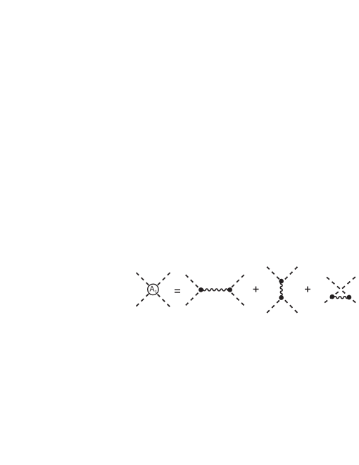
Figure 2: Tree amplitude $A_{t}$; the thick wavy lines incorporate the contact term of fig.1.

III s-channel loops

We work in the linear model and construct the dynamical features of the scalar resonance by considering only iterated contributions from a single loop. In this approximation, the dressed propagator is determined by the three diagrams shown in fig.3a. The last of them corresponds to a composite Dyson series and includes all possible iterations of the $\pi\pi$ tree amplitude, as represented in fig.3b.

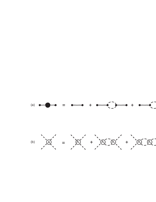
Figure 3: (a) Full resonance propagator; (b) $s$-channel unitarized $\pi\pi$ amplitude.

In this work we are mostly interested in exploring the behavior of coupled resonances. With this purpose in mind, we make a simplifying approximation and consider only the amplitude associated with the first diagram on the r.h.s. of fig.2, which is denoted by $A_{t}\equiv A_{t}(s)$ and given by eq.(9), for $x=s$. It is worth recalling, however, that the diagrams in the $t$ and $u$ channels also do play a visible role, as discussed in refs.BBWL and AS . The single loop contribution to the $\pi\pi$ scattering amplitude is given by

$$A_{1}(s)=A_{t}\left[-\Omega\right]A_{t}\;,$$ (11)

where the function

$$\Omega(s)=-\;\frac{3}{32\pi^{2}}\left[L+\Lambda_{\infty}\right]$$ (12)

contains an infinite constant $\Lambda_{\infty}$ and a finite component $L(s)$. The latter can be evaluated analytically and is given by

$$\bullet\;0\leq s<4\mu^{2}\rightarrow L(s)=-\;2\;\frac{\sqrt{4\mu^{2}-s}}{\sqrt{s}}\;\tan^{-1}\left[\frac{\sqrt{s}}{\sqrt{4\mu^{2}-s}}\right]\;,$$ (13)

$$\bullet\;4\mu^{2}\leq s\rightarrow L(s)=\frac{\sqrt{s-4\mu^{2}}}{\sqrt{s}}\;\left\{\ln\left[\frac{\sqrt{s}-\sqrt{s-4\mu^{2}}}{\sqrt{s}+\sqrt{s-4\mu^{2}}}\right]+i\;\pi\right\}\;.$$ (14)

The behavior of the function $L(s)$ is displayed in fig. 4, where it is possible to notice a cusp at $s=4\mu^{2}$.

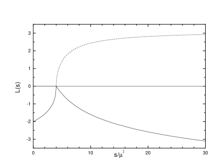
Figure 4: Function $L(s)$, that determines the self energy associated with the loop.

In the linear $\sigma$-model beyond tree level, loops bring infinities which must be removed consistently. The renormalization of the $\sigma$-model was discussed by Lee and collaborators BBWL ; BWL and reviewed in a pedagogical way in ref.PS . In order to keep only the essential features of our discussion, we note that the dynamical scalar mass can be cut along a $\pi\pi$ loop, whereas the pion mass can be cut along a $\pi\sigma$ loop. As the latter is heavier, we assume that changes in the pion mass can be neglected at the energy scale one is working at. The lifting of this restriction is straightforward, but would require a considerable increase in the algebraic effort. Since at one-loop level the wave function renormalization is finitePS , the elimination of $\Lambda_{\infty}$ from eq.(12) is performed by making $m\rightarrow m_{0}$ and $\lambda\rightarrow\lambda_{0}$ in the linear lagrangian and rewriting it as

$${\cal{L}} = \frac{1}{2}\left(\partial_{\mu}\sigma\;\partial^{\mu}\sigma+\partial_{\mu}\mbox{\boldmath$\pi$}\!\cdot\!\partial^{\mu}\mbox{\boldmath$\pi$}\right)-\frac{m^{2}}{2}\left(\sigma^{2}\!+\!\mbox{\boldmath$\pi$}^{2}\right)-\frac{\lambda}{4}\left(\sigma^{2}\!+\!\mbox{\boldmath$\pi$}^{2}\right)^{2}+f_{\pi}\,\mu^{2}\,\sigma$$ (15)

$$- \frac{\delta_{m}}{2}\left(\sigma^{2}\!+\!\mbox{\boldmath$\pi$}^{2}\right)-\frac{\delta_{\lambda}}{4}\left(\sigma^{2}\!+\!\mbox{\boldmath$\pi$}^{2}\right)^{2}\;,$$

with $\delta_{m}=m_{0}^{2}-m^{2}$ and $\delta_{\lambda}=\lambda_{0}-\lambda$. E expanding $\sigma$ around $f_{\pi}$, using the condition $\delta_{m}\!=\!-f_{\pi}^{2}\,\delta_{\lambda}$ associated with the constancy of $\mu^{2}$ and noting that tadpoles do not contribute by constructionPS , we find

$${\cal{L}} = \frac{1}{2}\left(\partial_{\mu}f\;\partial^{\mu}f-M_{\sigma}^{2}f^{2}\right)+\frac{1}{2}\left(\partial_{\mu}\mbox{\boldmath$\pi$}\!\cdot\!\partial^{\mu}\mbox{\boldmath$\pi$}-\mu^{2}\mbox{\boldmath$\pi$}^{2}\right)-\lambda\,f_{\pi}\,f\,\mbox{\boldmath$\pi$}^{2}-\lambda\,\mbox{\boldmath$\pi$}^{4}+\cdots$$ (16)

$$- \delta_{\lambda}\left(f_{\pi}^{2}\,f^{2}+f_{\pi}\,f\,\mbox{\boldmath$\pi$}^{2}+\mbox{\boldmath$\pi$}^{4}/4+\cdots\right)\;.$$

This result gives rise to the counterterm diagrams shown in fig. 5, which allow the factor $\Lambda_{\infty}$ in eq.(12) to be killed by a suitable choice of $\delta_{\lambda}$. We are then entitled to replace $\Omega(s)$ in eq.(11) by

$$\bar{\Omega}(s)=-\;\frac{3}{32\pi^{2}}\left[L+c\right]\;,$$ (17)

where $c$ is a yet undetermined constant. Denoting by $\bar{R}$ and $I$ the real and imaginary parts of $\bar{\Omega}$, the usual self energy insertion is written as

$$\bar{\Sigma}(s)=\gamma^{2}\left[\bar{R}+i\;I\right]\;.$$ (18)

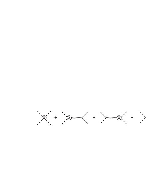
Figure 5: Counterterm structure for $A_{1}(s)$.

Considering all possible iterations of the two-pion loop, we construct the full $s-$channel $\pi\pi$ amplitude given in fig. 3b. This geometrical series can be summed and one finds

$$\bar{A}(s)=-\;\frac{\gamma^{2}}{s-{\cal{M}}_{A}^{2}+i\;M_{\sigma}\;\Gamma_{A}}\;,$$ (19)

with ${\cal{M}}_{A}^{2}(s)=M_{\sigma}^{2}+\gamma^{2}\bar{R}$ and $M_{\sigma}\Gamma_{A}(s)=\gamma^{2}I$. The scalar propagator, fig.3a, can be regularized by the same set of couterterms and reads

$$\bar{\Delta}(s)=\frac{1}{s-{\cal{M}}_{\Delta}^{2}+i\;M_{\sigma}\;\Gamma_{\Delta}}\;,$$ (20)

where

$${\cal{M}}_{\Delta}^{2}(s)=\mu^{2}+\frac{f_{\pi}^{2}(M_{\sigma}^{2}\!-\!\mu^{2})[f_{\pi}^{2}\!-\!(M_{\sigma}^{2}\!-\!\mu^{2})\bar{R}]}{[f_{\pi}^{2}\!-\!(M_{\sigma}^{2}\!-\!\mu^{2})\bar{R}]^{2}+(M_{\sigma}^{2}\!-\!\mu^{2})^{2}I^{2}}\;,$$

$$M_{\sigma}\Gamma_{\Delta}(s)=-\;\frac{f_{\pi}^{2}(M_{\sigma}^{2}\!-\!\mu^{2})^{2}\;I}{[f_{\pi}^{2}\!-\!(M_{\sigma}^{2}\!-\!\mu^{2})\bar{R}]^{2}+(M_{\sigma}^{2}\!-\!\mu^{2})^{2}I^{2}}\;.$$

The amplitude $\bar{A}$ and the propagator $\bar{\Delta}$ thus yield inequivalent definitions for the resonance mass and width, which correspond to different prescriptions for the determination of the parameter $c$ in eq.(17). We fix this constant by using the result for the $\pi\pi$ amplitude, for it is closer to observation. Imposing that the pole of $\bar{A}$ occurs at the physical mass $M_{\sigma}$, one finds $\bar{R}(M_{\sigma}^{2})=0\rightarrow c=-\Re L(M_{\sigma}^{2})$ and the running mass becomes ${\cal{M}}_{A}^{2}(s)=M_{\sigma}^{2}+\gamma^{2}[\bar{R}(s)-\bar{R}(M_{\sigma}^{2})]$, whereas the width reads

$$\Gamma_{A}(s)=\frac{3(s\!-\!\mu^{2})(M_{\sigma}^{2}\!-\!\mu^{2})}{32\pi\;f_{\pi}^{2}}\;\frac{\sqrt{s-4\mu^{2}}}{M_{\sigma}\sqrt{s}}\;\Theta(s\!-\!4\mu^{2})\;.$$ (22)

The signature of chiral symmetry in this problem is the factor $(s\!-\!\mu^{2})/f_{\pi}^{2}$, present in the functions $\gamma^{2}(s)$ and $\bar{\Sigma}(s)$. It implements the low energy theorem and is due to the use of eq.(6) as the main building block in the calculation. If one were to keep just the second term of eq.(5) in the evaluation of the two-pion loop contribution, it would be replaced by $(M_{\sigma}^{2}\!-\!\mu^{2})/f_{\pi}^{2}$. Thus, both procedures yield identical results at the pole, but correspond to rather different forms for the resonance width.

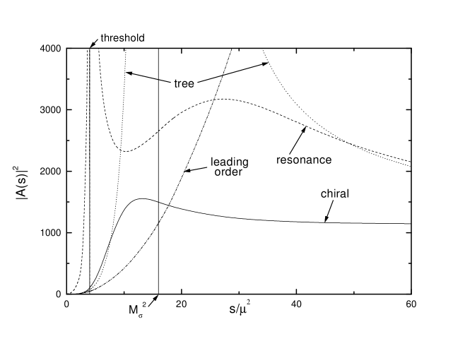
Figure 6: The functions $A(s)$ are the $\pi\pi$ amplitudes given by equations (2) (dot-dashed line), (6) (dotted line), (19) (continuous line) and by unitarizing just the $\sigma$ (dashed line).

In fig.6 we explore this this aspect of the problem, in the case of the function $|A(s)|^{2}$, for the choice $M_{\sigma}=4\mu$. The use of eq.(2) yields the leading order curve, an unbound parabola which blows up at large energies. The inclusion of the resonance as in eq.(6) gives rise to the tree curve. The chiral curve, given by eq.(19), is obtained by iterating the tree amplitude by means of two-pion loops. Finally, the resonance curve is derived by iterating just the second term of eq.(5) and then adding the first one. Inspecting this figure, one learns that the last procedure violates badly chiral symmetry, since it gives rise to a result which does not tend to the leading order one when $s\rightarrow 0$, as predicted by the low-energy theorems.

The reason for this kind of deviation can be found in fig.7, which shows the behaviors of the real and imaginary parts of the chiral and resonance amplitudes, together with the corresponding leading order and tree contributions. It is possible to notice that, at low-energies, the leading order, tree and chiral results stay close together, indicating that loop contributions are small. On the other hand, when one iterates just the second term of eq.(5), loop contributions are rather large and compatibility with the low-energy theorem is lost.

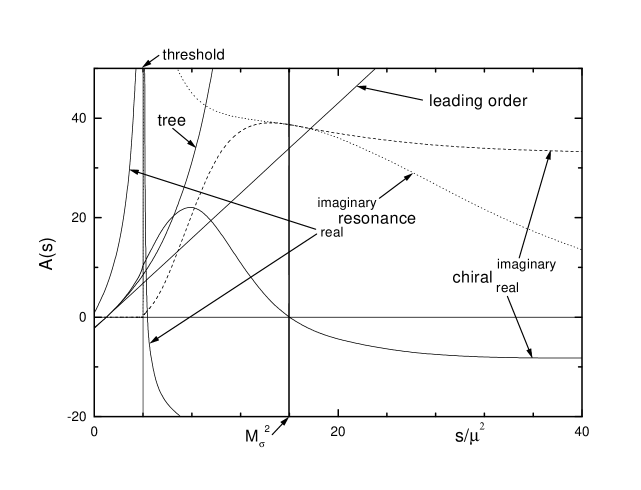
Figure 7: Real and imaginary parts of the $\pi\pi$ amplitude $A(s)$; the meanings of the labels are the same of fig.6.

IV $K$-matrix unitarization

A popular alternative procedure for unitarizing amplitudes is based on the so called $K$-matrix formalism. A resonance has a well defined isospin and it is useful to rewrite the generic $\pi\pi$ scattering amplitude as

$$T_{\pi\pi}=T_{0}(s,t,u)\;P_{0}+T_{1}(s,t,u)\;P_{1}+T_{2}(s,t,u)\;P_{2}\;,$$ (23)

where $P_{I}$ is the projector into the channel with total isospin $I$. The amplitudes $T_{I}$ are translated into the $A(x)$ of eq.(1) byGL

$$T_{0}=3\;A(s)+A(t)+A(u)\;,\;\;\;\;\;\;T_{1}=A(t)-A(u)\;,\;\;\;\;\;\;T_{2}=A(t)+A(u)\;.$$ (24)

In this work we neglect $t$ and $u$ channel effects and the scalar-isoscalar non-relativistic kernel for identical particles is related to the relativistic tree amplitude by

$$K(s)=\frac{3}{2}\;\frac{A_{t}}{8\pi\sqrt{s}}\;.$$ (25)

The on-shell iteration of this kernel yields the scattering amplitude $f$, which is given by

$$f=K/(1-iqK)\;,$$ (26)

where $q=\sqrt{s/4-\mu^{2}}$ is the center of mass momentum. Using $qK=\tan\delta$, one finds the usual phase shift parametrization for $f$. The relativistic counterpart of (26) reads

$$\bar{A}_{K}(s)=\frac{A_{t}}{1-i(3\sqrt{s\!-\!4\mu^{2}}\;A_{t}/32\pi\sqrt{s})}\;.$$ (27)

and, using eq.(9), we find

$$\bar{A}_{K}(s)=-\;\frac{\gamma^{2}}{s-M_{\sigma}^{2}+i\;M_{\sigma}\;\Gamma_{A}}\;.$$ (28)

In other words, one recovers the amplitude $\bar{A}(s)$ given by (19), with $\bar{R}=0$. This is expected since, as it is well known, $K\!\!-$matrix unitarization gives rise to a width, but does not renormalize the mass. In fig.8 we compare the functions $|\bar{A}(s)|^{2}$ and $|\bar{A}_{K}(s)|^{2}$, in order to show that the $K\!\!-$matrix formalism does produce a rather decent approximation for the explicit loop calculation, at a considerably lower algebraic cost.

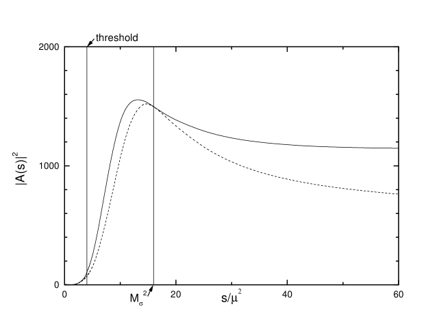
Figure 8: The functions $A(s)$ are the $\pi\pi$ amplitudes given by equations (19) (continuous line) and (28) (dashed line).

V extended $\sigma-$model

We now consider the problem of generalizing the linear $\sigma-$model, so that it could encompass two resonances. With this purpose in mind, we introduce a second scalar-isoscalar field $\xi$, which is assumed to be a chiral scalar. In other words, this new field is invariant under both isospin and axial transformations of the group $SU(2)\times SU(2)$. This allows its physical content to be compatible with realizations outside the $SU(2)$ sector such as, for instance, $s\bar{s}$ or glueball states.

In order to preserve renormalizability, we avoid couplings with negative dimensions and add two new chiral invariant terms to the ${\cal{L}}_{\sigma}$ of eq.(3). The two-resonance lagrangian becomes

$${\cal{L}}_{\sigma\xi}={\cal{L}}_{\sigma}+\frac{1}{2}\left(\partial_{\mu}\xi\;\partial^{\mu}\xi-M_{\xi}^{2}\,\xi^{2}\right)+g\,\xi\,\left(\sigma^{2}+\mbox{\boldmath$\pi$}^{2}\right)\;,$$ (29)

where $M_{\xi}$ is the $\xi$ mass and $g$ is a coupling constant. When the $\sigma$ is reexpressed in terms of the fluctuation $f$, the new interaction lagrangian gives rise to a contribution linear in $\xi$, indicating that this field also has a classical component, denoted by $e$. Writing $\sigma=f_{\pi}+f$ and $\xi=e+\epsilon$, we find

$${\cal{L}}_{\sigma\xi} = \left[-(m^{2}/2\!-\!ge)f_{\pi}^{2}\!-\!\lambda f_{\pi}^{4}/4\!+\!cf_{\pi}\right]+\left[-(m^{2}\!-\!2ge)f_{\pi}\!-\!\lambda f_{\pi}^{3}\!+\!c\right]f$$ (30)

$$+ \frac{1}{2}\left[\partial_{\mu}\mbox{\boldmath$\pi$}\!\cdot\!\partial^{\mu}\mbox{\boldmath$\pi$}-(m^{2}\!-\!2ge\!+\!\lambda f_{\pi}^{2})\,\mbox{\boldmath$\pi$}^{2}\right]+\frac{1}{2}\left[\partial_{\mu}f\;\partial^{\mu}f-(m^{2}\!-\!2ge\!+\!3\lambda f_{\pi}^{2})\,f^{2}\right]$$

$$- \left[\lambda f_{\pi}f(f^{2}+\mbox{\boldmath$\pi$}^{2})+\lambda\;\mbox{\boldmath$\pi$}^{4}/4+\cdots\right]+\left[-M_{\xi}^{2}e\!+\!gf_{\pi}^{2}\right]\epsilon$$

$$+ \frac{1}{2}\left(\partial_{\mu}\epsilon\;\partial^{\mu}\epsilon-M_{\xi}^{2}\,\epsilon^{2}\right)+g\,\epsilon\,\left(f^{2}+\mbox{\boldmath$\pi$}^{2}\right)+2\,g\,f_{\pi}\,f\,\epsilon\;.$$

The conditions $[-(m^{2}\!-\!2ge)f_{\pi}\!-\!\lambda f_{\pi}^{3}\!+\!c]=0$ and $[-M_{\xi}^{2}e\!+\!gf_{\pi}^{2}]=0$ for the free parameters allow the elimination of the linear terms in $f$ and $\epsilon$. The $\pi$ and $\sigma$ masses are

$$\mu^{2}=m^{2}\!-\!2ge\!+\!\lambda f_{\pi}^{2}\;,\;\;\;\;\;\;M_{\sigma}^{2}=\mu^{2}\!+\!2\lambda f_{\pi}^{2}\;.$$ (31)

The last term in eq.(30) corresponds to a mass mixing, which is eliminated by introducing new fields $\alpha$ and $\beta$, given by

$$\alpha=\cos\theta\,f+\sin\theta\,\epsilon\;,\;\;\;\;\;\;\beta=-\sin\theta\,f+\cos\theta\,\epsilon\;,$$ (32)

and choosing the angle $\theta$ such that $\tan 2\theta=4gf_{\pi}/(M_{\xi}^{2}\!-\!M_{\sigma}^{2})$. This yields

$$\cos^{2}\theta\;M_{\alpha}^{2}+\sin^{2}\theta\;M_{\beta}^{2}=M_{\sigma}^{2}\;,\;\;\;\;\;\;\sin^{2}\theta\;M_{\alpha}^{2}+\cos^{2}\theta\;M_{\beta}^{2}=M_{\xi}^{2}\;.$$ (33)

and allows the lagrangian to be written as

$${\cal{L}}_{\sigma\xi} = \frac{1}{2}\left[\partial_{\mu}\mbox{\boldmath$\pi$}\!\cdot\!\partial^{\mu}\mbox{\boldmath$\pi$}-\mu^{2}\,\mbox{\boldmath$\pi$}^{2}\right]+\frac{1}{2}\left[\partial_{\mu}\alpha\;\partial^{\mu}\alpha-M_{\alpha}^{2}\,\alpha^{2}\right]+\frac{1}{2}\left[\partial_{\mu}\beta\;\partial^{\mu}\beta-M_{\beta}^{2}\,\beta^{2}\right]$$ (34)

$$- f_{\pi}\left(\lambda_{\alpha}\;\alpha+\lambda_{\beta}\;\beta\right)\mbox{\boldmath$\pi$}^{2}-\lambda\;\mbox{\boldmath$\pi$}^{4}/4+\cdots$$

where the coupling constants $\lambda_{\alpha}$, $\lambda_{\beta}$ and $\lambda$ are completely determined by the masses and mixing angle as

$$\lambda_{\alpha}=\cos\theta\;\left(M_{\alpha}^{2}\!-\!\mu^{2}\right)/2f_{\pi}^{2}\;,\;\;\;\;\;\;\lambda_{\beta}=-\sin\theta\;\left(M_{\beta}^{2}\!-\!\mu^{2}\right)/2f_{\pi}^{2}\;,$$ (35)

$$\lambda=\left[\cos^{2}\theta\left(M_{\alpha}^{2}\!-\!\mu^{2}\right)+\sin^{2}\theta\left(M_{\beta}^{2}\!-\!\mu^{2}\right)\right]/2f_{\pi}^{2}\;.$$ (36)

The tree amplitude for $\pi\pi$ scattering is given by the diagrams of fig.9 and reads

$$A_{t}(x)=-2\;\lambda-\;\frac{4\;\lambda_{\alpha}^{2}\;f_{\pi}^{2}}{x-M_{\alpha}^{2}}-\;\frac{4\;\lambda_{\beta}^{2}\;f_{\pi}^{2}}{x-M_{\beta}^{2}}$$

$$=\frac{x\!-\!\mu^{2}}{f_{\pi}^{2}}\;\left[1-\cos^{2}\theta\;\frac{x\!-\!\mu^{2}}{x-M_{\alpha}^{2}}-\sin^{2}\theta\;\frac{x\!-\!\mu^{2}}{x-M_{\beta}^{2}}\right]\;.$$ (37)

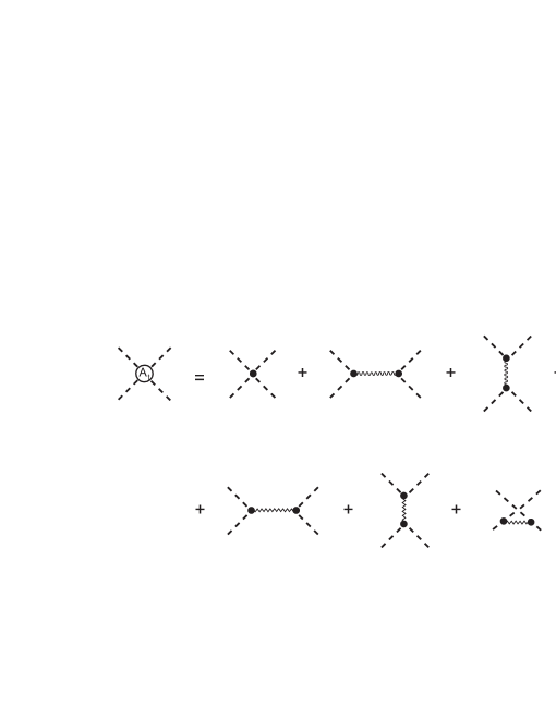
Figure 9: Tree amplitude $A_{t}$; dashed and thin wavy and zigzag lines represent pions and scalar resonances $\alpha$ and $\beta$.

This result corresponds to the generalization of eq.(6) and is consistent, as it must be, with the low energy theorem. As in the single resonance case, it is convenient to write the tree amplitude as

$$A_{t}(x)\equiv A_{t\alpha}(x)+A_{t\beta}(x)=-\;\frac{\gamma_{\alpha}^{2}}{x-M_{\alpha}^{2}}-\;\frac{\gamma_{\beta}^{2}}{x-M_{\beta}^{2}}\;,$$ (38)

with

$$\gamma_{\alpha}^{2}(x)=\cos^{2}\theta\,(x\!-\!\mu^{2})(M_{\alpha}^{2}\!-\!\mu^{2})/f_{\pi}^{2}\;,\;\;\;\;\;\;\ \gamma_{\beta}^{2}(x)=\sin^{2}\theta\,(x\!-\!\mu^{2})(M_{\beta}^{2}\!-\!\mu^{2})/f_{\pi}^{2}\;,$$ (39)

and reexpress the diagrams of fig.9 as in fig.10, where the thick lines now incorporate the contributions from the four-pion contact interaction and the functions $\gamma_{i}^{2}$ correspond to effective couplings.

.

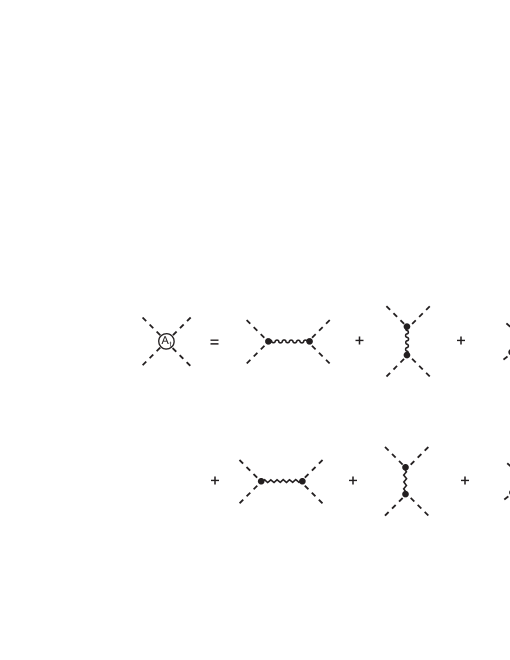
Figure 10: Tree amplitude $A_{t}$; the thick wavy and zigzag lines incorporate the contact term of fig.9.

VI coupled resonances

In the case of two scalar resonances $\alpha$ and $\beta$, which can couple through a two-pion intermediate state, one has to consider the four two-point functions displayed in fig.11a. The structures of these functions are given in figs.11b and depend on the full elastic $\pi\pi$ amplitude.

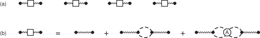
Figure 11: (a) Coupled resonance propagators and (b) their dynamical structures; dashed and thin wavy and zigzag lines represent pions and scalar resonances $\alpha$ and $\beta$.

As in the single resonance case, the $\pi\pi$ amplitude is obtained by iterating the tree result from the previous section. The first iteration of eq.(38) yields

$$A_{1}(s)=\left[A_{t\alpha}+A_{t\beta}\right]\left[-\Omega\right]\left[A_{t\alpha}+A_{t\beta}\right]\;,$$ (40)

where $\Omega$ is given by eq.(12) and contains a divergence that needs to be removed by renormalization. The same formal manipulations used in section 3 allow couterterms to be generated in the two-resonance lagrangian, eq.(29), and the regularized version of $A_{1}$ reads

$$\bar{A}_{1}(s)=\sum_{i=\alpha}^{\beta}\sum_{j=\alpha}^{\beta}A_{ti}\left[-\bar{\Omega}_{ij}\right]A_{tj}\;,$$ (41)

with

$$\bar{\Omega}_{ij}(s)=-\;\frac{3}{32\pi^{2}}\left[L+c_{ij}\right]\;.$$ (42)

The self-energy associated with a particular interaction is given by

$$\bar{\Sigma}_{ij}(s)=\gamma_{i}\;\gamma_{j}\left[\bar{R}_{ij}+i\;I\right]\;.$$ (43)

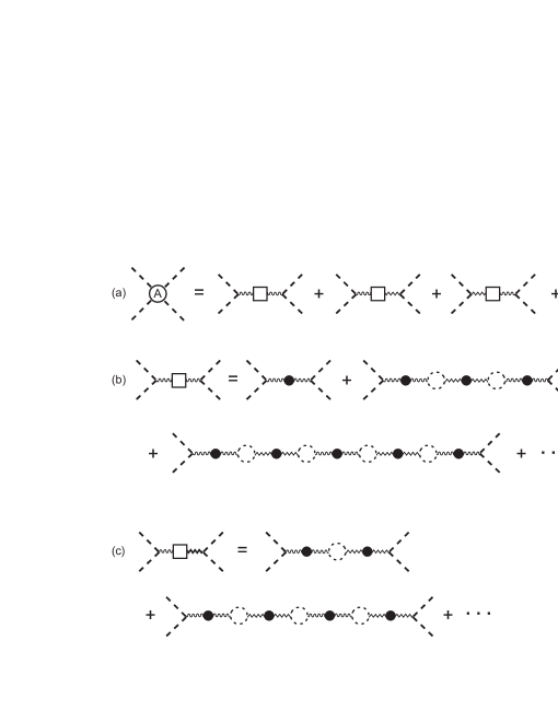
Figure 12: (a) Coupled resonance contribution to the $\pi\pi$ amplitude and (b, c) partial contributions. The meaning of thick wavy and zigzag lines is given in fig. 10.

The iteration of this amplitude to all orders gives rise to the structure shown in fig.12a, which contains four sub amplitudes, denoted by $\bar{A}_{ij}$. In order to construct these functions, we first evaluate the single resonance contributions from fig.12b, and recover result given in eq.(19). We then assemble all possible combinations of these results, as in figs.12c, and find the diagonal and off-diagonal amplitudes as

$$\bar{A}_{\alpha\alpha}(s)=\frac{-\gamma_{\alpha}^{2}\;[s\!-\!M_{\beta}^{2}\!-\!\gamma_{\beta}^{2}(\bar{R}_{\beta\beta}+iI)]}{D+i\;G}\;.$$ (44)

$$\bar{A}_{\alpha\beta}(s)=\frac{-\gamma_{\alpha}^{2}\;\gamma_{\beta}^{2}\;(\bar{R}_{\alpha\beta}+iI)}{D+i\;G}\;.$$ (45)

with

$$D(s) = \left(s\!-\!M_{\alpha}^{2}\!-\!\gamma_{\alpha}^{2}\,\bar{R}_{\alpha\alpha}\right)\left(s\!-\!M_{\beta}^{2}\!-\!\gamma_{\beta}^{2}\,\bar{R}_{\beta\beta}\right)-\gamma_{\alpha}^{2}\gamma_{\beta}^{2}\left(\bar{R}_{\alpha\beta}\right)^{2}\;,$$ (46)

$$G(s) = -\gamma_{\alpha}^{2}\,(s\!-\!M_{\beta}^{2})-\gamma_{\beta}^{2}\,(s\!-\!M_{\alpha}^{2})+\gamma_{\alpha}^{2}\,\gamma_{b}^{2}\,(\bar{R}_{\alpha\alpha}+\bar{R}_{\beta\beta}-2\,\bar{R}_{\alpha\beta})\;.$$ (47)

The expression for $\bar{A}_{\beta\beta}$ is obtained by making $(\alpha\leftrightarrow\beta)$ in eq.(44). The evaluation of the full $s-$channel $\pi\pi$ amplitude produces

$$\bar{A}(s)=\frac{G}{D+i\;G\;I}\;.$$ (48)

This result allows the construction of resonance propagators. However, the resulting expressions are rather messy and will not be quoted. In order to determine the couterterms $c_{ij}$ in eq.(42), we use directly the $\pi\pi$ amplitude. Imposing that the resonances decouple at their poles, we find $(\bar{R}_{\alpha\alpha}+\bar{R}_{\beta\beta}-2\,\bar{R}_{\alpha\beta})=0$. The function $G(s)$ becomes proportional to the tree amplitude $A_{t}(s)$ given by eq.(38) and the unitarized amplitude can be written as

$$\bar{A}(s)=\frac{A_{t}(s)}{[D/(s\!-\!M_{\alpha}^{2})(s\!-\!M_{\beta}^{2})]+i\;A_{t}(s)\;I}\;.$$ (49)

This result shows that the zeroes of $\bar{A}(s)$ and $A_{t}(s)$ coincide, enforcing the theorem given by TörnqvistTor , which states that ”a zero in the partial wave amplitude in the physical region remains a zero after unitarization”. The zeroes of $A_{t}(s)$ occur at $s=\mu^{2}$ and the point

$$s_{1}=\frac{M_{\alpha}^{2}\,M_{\beta}^{2}-\mu^{2}(M_{\beta}^{2}\cos^{2}\theta\!+\!M_{\alpha}^{2}\sin^{2}\theta)}{M_{\alpha}^{2}\cos^{2}\theta+M_{\beta}^{2}\sin^{2}\theta-\mu^{2}}\;,$$ (50)

with $M_{\alpha}^{2}<s_{1}<M_{\beta}^{2}$. In principle, the position of this point could be obtained from analyses of empirical data and the value of the mixing angle $\theta$ would be related to the masses by

$$\tan^{2}\theta=\frac{(M_{\beta}^{2}\!-\!s_{1})\,(M_{\alpha}^{2}\!-\!\mu^{2})}{(s_{1}\!-\!M_{\alpha}^{2})\,(M_{\beta}^{2}\!-\!\mu^{2})}\;.$$ (51)

Imposing $D(M_{\alpha}^{2})=D(M_{\beta}^{2})=0$, one finds the conditions

$$c_{\alpha\alpha}\!-\!c_{\beta\beta}=\frac{64\pi^{2}f_{\pi}^{2}(M_{\alpha}^{2}\!-\!M_{\beta}^{2})}{3(M_{\alpha}^{2}\!-\!\mu^{2})(M_{\beta}^{2}\!-\!\mu^{2})}\left\{1\!\pm\!\sqrt{1\!+\!\frac{3(M_{\alpha}^{2}\!-\!\mu^{2})(M_{\beta}^{2}\!-\!\mu^{2})\Re\left[L(M_{\alpha}^{2})\!-\!L(M_{\beta}^{2})\right]}{32\pi^{2}f_{\pi}^{2}(M_{\alpha}^{2}\!-\!M_{\beta}^{2})}}\right\}\;,$$ (52)

$$c_{\alpha\alpha}=-\Re\left[L(M_{\alpha}^{2})\cos^{2}\theta\!+\!L(M_{\beta}^{2})\sin^{2}\theta\right]+(c_{\alpha\alpha}\!-\!c_{\beta\beta})\sin^{2}\theta\;,$$ (53)

$$c_{\beta\beta}=-\Re\left[L(M_{\alpha}^{2})\cos^{2}\theta\!+\!L(M_{\beta}^{2})\sin^{2}\theta\right]-(c_{\alpha\alpha}\!-\!c_{\beta\beta})\cos^{2}\theta\;,$$ (54)

which allow the constants $c_{\alpha\alpha}$ and $c_{\beta\beta}$ to be fixed.

The dependence of the unitarized amplitude $|\bar{A}(s)|^{2}$ on the mixing angle $\theta$ is shown fig.13, for the choices $M_{\alpha}=4\mu$ and $M_{\beta}=8\mu$.

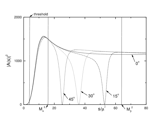
Figure 13: The function $\bar{A}(s)$ is the unitarized amplitude given by eq.(49) and the angles quoted represent possible mixings between resonances $\alpha$ and $\beta$.

VII summary and general results

In this work we have used the linear $\sigma$-model in order to study how chiral symmetry affects amplitudes incorporating scalar resonances. Most of our qualitative results confirm, in a lagrangian framework, those derived by TörnqvistTor about ten years ago, using a unitarized quark model.

One of the implications of chiral symmetry is that the elastic $\pi\pi$ amplitude must vanish at the subthreshold point $s=\mu^{2}$, where $\mu$ is the pion mass. As this point is close to the threshold at $s=4\mu^{2}$, the physical amplitude becomes strongly constrained in the low-energy region. This aspect of the problem is clearly visible in figs. 6 and 7, for the single resonance case. From a technical point of view, this happens because the chiral constraint is already present in the tree amplitude, given by eqs.(6), (9) and (10). As the unitarization procedure cannot change the position of the chiral zero, it becomes an essential feature of the full result.

The discussion following eq.(19) shows that pion loops do affect both the real and imaginary parts of the denominator of the unitarized amplitude. However, the neglect of these effects in the real part, which correspond to more complicated expressions, yields a decent approximation for the full result, as one learns from fig. 8. Thus, in exploratory studies, one may keep just the pion loop contributions to the imaginary term, which are rather simple. The single resonance width is given in eq.(22) and it is worth noting that it incorporates a factor $1/2!$ due to the exchange symmetry of the intermediate two-pion state.

In section 5 we have produced an extension of the linear $\sigma$-model aimed at including a second resonance and found out that the tree $\pi\pi$ amplitude can be written as

$$A_{t}(s)=\frac{s\!-\!\mu^{2}}{f_{\pi}^{2}}\;\left[1-\cos^{2}\theta\,\frac{s\!-\!\mu^{2}}{s\!-\!M_{\alpha}^{2}}-\sin^{2}\theta\,\frac{s\!-\!\mu^{2}}{s\!-\!M_{\beta}^{2}}\right]\;,$$ (55)

where $\theta$ is a mixing angle. For $M_{\alpha}=M_{\beta}$, one recovers eq.(6), for the single resonance case. This structure gives rise to a second zero for the tree amplitude, which occurs at a point $s_{1}$, such that $M_{\alpha}^{2}<s_{1}<M_{\beta}^{2}$. The behavior of this zero as a function of $\theta$ can be found in both eq.(50) and fig. 13.

When the effects of pion loops over the real part of the amplitude denominator are neglected, the relationship between the tree and unitarized amplitudes, given by eq.(49), becomes particularly simple:

$$\bar{A}(s)=\frac{A_{t}(s)}{1-i[3\sqrt{s\!-\!4\mu^{2}}\;A_{t}(s)/32\pi\sqrt{s}]}\;.$$ (56)

This result, derived in the two-resonance case, is very general and holds for any number of resonances. It corresponds to the iteration of the tree amplitude as a whole and is not sensitive to its internal structure. Here, again, the iteration includes a $1/2!$ statistical factor.

In order to extend our results to the case of $N$ coupled scalar resonances, we propose to generalize the chiral tree amplitude by means of the expression

$$A_{t}(s)=\frac{s\!-\!\mu^{2}}{f_{\pi}^{2}}\;\left[1-\lambda_{1}\,\frac{s\!-\!\mu^{2}}{s\!-\!M_{1}^{2}}-\cdots-\lambda_{N}\,\frac{s\!-\!\mu^{2}}{s\!-\!M_{N}^{2}}\right]\;,$$ (57)

where the $\lambda_{i}$ are weights constrained by the condition $1=\lambda_{1}+\cdots\lambda_{N}$. This amplitude has $N$ zeroes. The first of them occurs at $s=\mu^{2}$ and is due to chiral symmetry. The remaining ones are Törnqvist zeroes and occur at the points $s_{1},\cdots,s_{N-1}$, between the various resonances. In principle, the location of these points could be determined empirically and used to express all the weights $\lambda_{i}$ as functions of the masses $M_{i}$, as in eq.(51). Feeding this information back into eqs.(57) and (55), one ends up with an expression for the unitarized amplitude which depends only on unknown masses, which can be extracted from fits to data.

The results presented in this work were derived in the framework of the linear $\sigma$-model and, to some extent, depend on this choice. On the other hand, they also convey a more general content, namely that the parametrization of the widths of scalar resonances coupled to pions, associated with the imaginary term in eq.(56), must always include a factor $(s\!-\!\mu^{2})/f_{\pi}^{2}$, in order to be compatible with chiral symmetry.

At present, we are considering the inclusion of $K$ and $\eta$ mesons in our results.

Acknowledgement
It is our pleasure to thank Ignacio Bediaga for several conversations about experimental aspects of scalar resonances.

References

(1) F. E. Close, preprint hep-ph/0311087, AIP Conf. Proc. 717, 919 (2004).
(2) N. A. Törnqvist, Z. Phys. C68, 647 (1995).
(3) M. Svec, Phys. Rev. D64, 096003 (2001).
(4) E791 Collaboration, E. M. Aitala et al., Phys. Rev. Lett. 86, 770 (2001).
(5) E791 Collaboration, E. M. Aitala et al., Phys. Rev. Lett. 89, 121801 (2002).
(6) CLEO Collabotration, H. Muramatsu et al., Phys. Rev. Lett. 89, 251802 (2002).
(7) Belle Collaboration, K. Abe et al. preprint hep-ex/0308043.
(8) BaBar Collaboration, B. Aubert et al. preprint hep-ex/0408088.
(9) KLOE Collaboration, A. Aloisio et al. Phys. Lett. B537, 21 (2002).
(10) BES Collaboration, J-Z. Bai et al., preprint hep-ex/0404016.
(11) BaBar Collaboration, B. Aubert et al. preprint hep-ex/0408032.
(12) S. Weinberg, Phys. Rev. 166, 1568 (1968).
(13) C. M. Maekawa and M. R. Robilotta, Phys. Rev. C57, 2839 (1998).
(14) J. L. Basdevant and B. W. Lee, Phys. Rev. D2, 1680 (1970).
(15) N. N. Achasov and G. N. Shestakov, Phys. Rev. D49, 5779 (1994).
(16) B. W. Lee, Nucl. Phys. B9, 649 (1969);
B. W. Lee and J. L. Gervais, Nucl. Phys. B12, 627 (1969); B.
W. Lee, Chiral Dynamics, Gordon and Breach, New York, 1972.
(17) M. E. Peskin and D. V. Schroeder, An Introduction to Quantum Field Theory,
Addison-Wesley, 1995, chap.11.
(18) J. Gasser and H. Leutwyler, Ann. Phys. (N.Y.) 158, 142 (1984).