Abstract

Inclusive cross sections for pion production in proton-proton collisions are calculated for the first time based on unintegrated parton (gluon, quark, antiquark) distributions (uPDF). We use Kwieciński uPDF’s and phenomenological fragmentation functions from the literature. In addition to the $gg\to g$ diagram used recently for applications at RHIC we include also $gq\to q$ and $qg\to q$ diagrams. We find that the new contributions are comparable to the purely gluonic one at midrapidities and dominate in the fragmentation region. The new mechanisms are responsible for $\pi^{+}-\pi^{-}$ asymmetry. We discuss how the asymmetry depends on $x_{F}$ and $p_{t}$. Inclusive distributions in $x_{F}$ (or rapidity) and transverse momentum for partons and pions are shown for illustration. In contrast to standard collinear approach in our approach the range of applicability can be extended towards much lower transverse momenta.

PACS: 12.38.Bx, 13.85.Hd, 13.85.Ni

1 Introduction

The distributions of mesons at large transverse momenta in $pp$ or $p\bar{p}$ collisions are usually calculated in the framework of perturbative QCD using collinear factorization (see e.g. [1, 2, 3, 4]). While the shape at transverse momenta larger than 2-4 GeV can be relatively well explained, the difference between the data and the lowest-order computation is quantified in terms of a so-called K-factor, independent quantity for each energy [4]. The K-factor is found to systematically decrease with growing energy [5]. In order to extend the calculation towards lower values of meson transverse momenta it was suggested to add an extra Gaussian distribution in transverse momentum [6, 7, 8] . In this approach the standard collinear integrals are replaced as:

$$dx\;p(x,\mu^{2})\to dxd^{2}k_{t}\;g(k_{t})p(x,\mu^{2})\;,$$ (1)

where the extra distribution function in transverse momentum is normalized to unity

$$\int d^{2}k_{t}\;g(k_{t})=1.$$ (2)

It is customary to use Gaussian distributions for $g(k_{t})$. It becomes clear that this procedure is effective in the following sense. The transverse momentum originates either from the nonperturbative “really internal” momentum distributions of partons in nucleons (of the order of a fraction of GeV) and/or is generate dynamically as the inital state radiation process (of the order of GeV). In principle, the second component may depend on the values of longitudinal momentum fractions $x_{1}$ and/or $x_{2}$. The formalism used by us in the present paper will include both these effects separately and explicitly.

The recent results from RHIC (see e.g. [13]) have attracted a renewed interest in better understanding the dynamics of particle production, not only in nuclear collisions. Quite different approaches have been used to describe the particle spectra from the nuclear collisions [14]. The model in Ref.[10] with an educated guess for UGD describes surprisingly well the whole charged particle rapidity distribution by means of gluonic mechanisms only. Such a gluonic mechanism would lead to identical production of positively and negatively charged hadrons. The recent results of the BRAHMS experiment concerning heavy ion collisions [15] show that the $\pi^{-}/\pi^{+}$ and $K^{-}/K^{+}$ ratios differ from unity. This put into question the successful description of Ref.[10]. In the light of this experiment, it becomes obvious that the large rapidity regions have more complicated flavour structure. At lower energies these ratios are known to differ from unity drastically [28].

In Ref.[11] one of us has calculated inclusive pion spectra in proton-proton collisions based on different models of unintegrated gluon distributions taken from the literature. In the present paper in addition to the $gg\to g$ mechanism we include also $q_{f}g\to q_{f}$ and $gq_{f}\to q_{f}$ mechanisms and similar ones for antiquarks in order to obtain a fully consistent description.

Many unintegrated gluon distributions in the literature are ad hoc parametrizations of different sets of experimental data rather than derived from QCD. An example of a more systematic approach, making use of familiar collinear distributions can be found in Ref.[17]. Recently Kwieciński and collaborators [18, 19, 20] have shown how to solve the so-called CCFM equations by introducing unintegrated parton distributions in the space conjugated to the transverse momenta [18]. We present first results for pion production based on unintegrated parton (gluon, quark, antiquark) distributions obtained by solving a set of coupled equations developed by Kwieciński and collaborators. Recently these parton distributions were tested for inclusive gauge boson production in proton-antiproton collisions [21] and for charm-anticharm correlations in photoproduction [22]. While in the first process one tests mainly quark and antiquark distributions at scales $\mu^{2}\sim M_{W}^{2},M_{Z}^{2}$, in the second reaction one tests mainly gluon distributions at scales $\mu^{2}\sim m_{c}^{2}$. In comparison to those reactions in the present application one tests both gluon as well as quark and antiquark distributions in a “more nonperturbative” region of smaller scales of the order down to $\mu\sim p_{t}$(parton) $\sim$ 0.5 - 1.0 GeV, which corresponds to pion transverse momenta $p_{t}$(pion) $\sim$ 0.25 - 0.5 GeV. This is a region where perturbative and nonperturbative effects are believed to mix up and the application of the pQCD is doubtful. On the other hand, this is an interesting region of phase space responsible for the bulk of hadronic production. We shall discuss how far down to small pion transverse momenta one can apply the present approach.

Some preliminary results of the present study were presented at a conference [12].

2 Kwieciński unintegrated parton distributions

Kwieciński has shown that the evolution equations for unintegrated parton distributions takes a particularly simple form in the variable conjugated to the parton transverse momentum. The two possible representations are interrelated via Fourier-Bessel transform

$$\begin{split}&{f_{k}(x,\kappa_{t}^{2},\mu^{2})}=\int_{0}^{\infty}db\;bJ_{0}(\kappa_{t}b){{\tilde{f}}_{k}(x,b,\mu^{2})}\;,\\ &{{\tilde{f}}_{k}(x,b,\mu^{2})}=\int_{0}^{\infty}d\kappa_{t}\;\kappa_{t}J_{0}(\kappa_{t}b){f_{k}(x,\kappa_{t}^{2},\mu^{2})}\;.\end{split}$$ (3)

The index k above numerates either gluons (k=0), quarks (k$>$ 0) or antiquarks (k$<$ 0). In the impact-parameter space the Kwieciński equation takes the following simple form

$$\begin{split}{\partial{\tilde{f}_{NS}(x,b,\mu^{2})}\over\partial\mu^{2}}&={\alpha_{s}(\mu^{2})\over 2\pi\mu^{2}}\int_{0}^{1}dz\,P_{qq}(z)\bigg{[}\Theta(z-x)\,J_{0}((1-z)\mu b)\,{\tilde{f}_{NS}\left({x\over z},b,\mu^{2}\right)}\\ &-{\tilde{f}_{NS}(x,b,\mu^{2})}\bigg{]}\;,\\ {\partial{\tilde{f}_{S}(x,b,\mu^{2})}\over\partial\mu^{2}}&={\alpha_{s}(\mu^{2})\over 2\pi\mu^{2}}\int_{0}^{1}dz\bigg{\{}\Theta(z-x)\,J_{0}((1-z)\mu b)\bigg{[}P_{qq}(z)\,{\tilde{f}_{S}\left({x\over z},b,\mu^{2}\right)}\\ &+P_{qg}(z)\,{\tilde{f}_{G}\left({x\over z},b,\mu^{2}\right)}\bigg{]}-[zP_{qq}(z)+zP_{gq}(z)]\,{\tilde{f}_{S}(x,b,\mu^{2})}\bigg{\}}\;,\\ {\partial{\tilde{f}_{G}(x,b,\mu^{2})}\over\partial\mu^{2}}&={\alpha_{s}(\mu^{2})\over 2\pi\mu^{2}}\int_{0}^{1}dz\bigg{\{}\Theta(z-x)\,J_{0}((1-z)\mu b)\bigg{[}P_{gq}(z)\,{\tilde{f}_{S}\left({x\over z},b,\mu^{2}\right)}\\ &+P_{gg}(z)\,{\tilde{f}_{G}\left({x\over z},b,\mu^{2}\right)}\bigg{]}-[zP_{gg}(z)+zP_{qg}(z)]\,{\tilde{f}_{G}(x,b,\mu^{2})}\bigg{\}}\;.\end{split}$$ (4)

We have introduced here the short-hand notation

$$\begin{split}\tilde{f}_{NS}&=\tilde{f}_{u}-\tilde{f}_{\bar{u}},\;\;\tilde{f}_{d}-\tilde{f}_{\bar{d}}\;,\\ \tilde{f}_{S}&=\tilde{f}_{u}+\tilde{f}_{\bar{u}}+\tilde{f}_{d}+\tilde{f}_{\bar{d}}+\tilde{f}_{s}+\tilde{f}_{\bar{s}}\;.\end{split}$$ (5)

The unintegrated parton distributions in the impact factor representation are related to the familiar collinear distributions as follows

$$\tilde{f}_{k}(x,b=0,\mu^{2})=\frac{x}{2}p_{k}(x,\mu^{2})\;.$$ (6)

On the other hand, the transverse momentum uPDF’s are related to the integrated distributions as

$$xp_{k}(x,\mu^{2})=\int_{0}^{\infty}d\kappa_{t}^{2}\;f_{k}(x,\kappa_{t}^{2},\mu^{2})\;.$$ (7)

While physically $f_{k}(x,\kappa_{t}^{2},\mu^{2})$ should be positive, there is no obvious reason for such a limitation for $\tilde{f}_{k}(x,b,\mu^{2})$.

In the following we use leading-order parton distributions from ref.[29] as the initial condition for QCD evolution. The set of integro-differential equations in b-space was solved by the method based on the discretisation made with the help of the Chebyshev polynomials (see e.g. [20]). Then the unintegrated parton distributions were put on a grid in $x$, $b$ and $\mu^{2}$ and the grid was used in practical applications for Chebyshev interpolation (see next section).

3 Inclusive cross sections for partons

The approach proposed by Kwieciński is very convenient to introduce the nonperturbative effects like internal (nonperturbative) transverse momentum distributions of partons in nucleons. It seems reasonable, at least in the first approximation, to include the nonperturbative effects in the factorizable way

$$\tilde{f}_{q}(x,b,\mu^{2})=\tilde{f}_{q}^{CCFM}(x,b,\mu^{2})\cdot F_{q}^{np}(b)\;.$$ (8)

The form factor responsible for the nonperturbative effects must be normalized such that

$$F^{NP}(b=0)=1$$ (9)

in order not to spoil the relation (6). In the following, for simplicity, we use a flavour and $x$-independent form factor

$$F_{q}^{np}(b)=F^{np}(b)=\exp\left(-\frac{b^{2}}{4b_{0}^{2}}\right)\;$$ (10)

which describes the nonperturbative effects. The Gaussian form factor in $b$ means also a Gaussian initial momentum distribution $\propto\exp(-k_{t}^{2}b_{0}^{2})$ (Fourier transform of a Gaussian function is a Gaussian function). Gaussian form factor is often used to correct collinear pQCD calculations for the so-called internal momenta. Other functional forms in $b$ are also possible.

The $gg\to g$ mechanism considered in the literature is not the only one possible. In Fig.1 we show two other leading order diagrams. They are potentially important in the so-called fragmentation region. The formulae for inclusive quark/antiquark distributions are similar to the formula for $gg\to g$ [16]. The formulae for all the processes mentioned are listed below:

for diagram A (gg$\to$g):

$$\frac{d\sigma^{A}}{dyd^{2}p_{t}}=\frac{16N_{c}}{N_{c}^{2}-1}{\frac{1}{p_{t}^{2}}}$$

$$\int\alpha_{s}({\Omega^{2}})\;{f_{g/1}(x_{1},\kappa_{1}^{2},\mu^{2})}\;{f_{g/2}(x_{2},\kappa_{2}^{2},\mu^{2})}$$

$$\delta^{(2)}(\vec{\kappa}_{1}+\vec{\kappa}_{2}-\vec{p}_{t})\;d^{2}\kappa_{1}d^{2}\kappa_{2}\;,$$ (11)

for diagram B₁ (q_f g $\to$ q_f):

$$\frac{d\sigma^{B_{1}}}{dyd^{2}p_{t}}=\frac{16N_{c}}{N_{c}^{2}-1}\left(\frac{4}{9}\right){\frac{1}{p_{t}^{2}}}$$

$$\sum_{f}\int\alpha_{s}({\Omega^{2}})\;{f_{q_{f}/1}(x_{1},\kappa_{1}^{2},\mu^{2})}\;{f_{g/2}(x_{2},\kappa_{2}^{2},\mu^{2})}$$

$$\delta^{(2)}(\vec{\kappa}_{1}+\vec{\kappa}_{2}-\vec{p}_{t})\;d^{2}\kappa_{1}d^{2}\kappa_{2}\;,$$ (12)

for diagram B₂ (g q_f $\to$ q_f):

$$\frac{d\sigma^{B_{2}}}{dyd^{2}p_{t}}=\frac{16N_{c}}{N_{c}^{2}-1}\left(\frac{4}{9}\right){\frac{1}{p_{t}^{2}}}$$

$$\sum_{f}\int\alpha_{s}({\Omega^{2}})\;{f_{g/1}(x_{1},\kappa_{1}^{2},\mu^{2})}\;{f_{q_{f}/2}(x_{2},\kappa_{2}^{2},\mu^{2})}$$

$$\delta^{(2)}(\vec{\kappa}_{1}+\vec{\kappa}_{2}-\vec{p}_{t})\;d^{2}\kappa_{1}d^{2}\kappa_{2}\;.$$ (13)

These seemingly 4-dimensional integrals can be written as 2-dimensional integrals after a siutable change of variables [11]

$$\int\;...\;\delta^{(2)}(\vec{\kappa}_{1}+\vec{\kappa}_{2}-\vec{p}_{t})\;d^{2}\kappa_{1}d^{2}\kappa_{2}=\int\;...\;\frac{d^{2}q_{t}}{4}\;.$$ (14)

The integrands of these “reduced” 2-dimensional integrals in $\vec{q}_{t}=\vec{\kappa_{1}}-\vec{\kappa_{2}}$ are generally smooth functions of $q_{t}$ and corresponding azimuthal angle $\phi_{q_{t}}$. In the following we use two different prescriptions for the factorization scale $\mu^{2}$:

• $\mu^{2}=p_{t}^{2}$ with freezing for $p_{t}^{2}<\mu^{2}$,

• $\mu^{2}=p_{t}^{2}+\mu_{0}^{2}$.

In Eqs.(11), (12) and (13) the longitudinal momentum fractions

$$x_{1/2}=\frac{\sqrt{p_{t}^{2}+m_{x}^{2}}}{\sqrt{s}}\exp(\pm y)\;,$$ (15)

where $m_{x}$ is the effective mass of the parton.

The sums in (12) and (13) run over both quarks and antiquarks. The argument of the running coupling constant $\Omega^{2}$ above was not specified explicitly yet. In principle, it can be $p_{t}^{2}$ or a combination of $p_{t}^{2}$, $\kappa_{1}^{2}$ and $\kappa_{2}^{2}$. In the standard transverse momentum representation it is reasonable to assume $\Omega^{2}=\min(p_{t}^{2},\kappa_{1}^{2},\kappa_{2}^{2})$ (see e.g. [11]). In the region of very small $p_{t}$ usually $p_{t}^{2}<\kappa_{1}^{2},\kappa_{2}^{2}$ and $\Omega_{2}=p_{t}^{2}$ is a good approximation.

Assuming for simplicity that $\Omega^{2}=\Omega^{2}(p_{t}^{2})$ or $p_{t}^{2}$ (function of transverse momentum squared of the “produced” parton, or simply transverse momentum squared) and taking the following representation of the $\delta$ function

$$\delta^{(2)}(\vec{\kappa_{1}}+\vec{\kappa_{2}}-\vec{p}_{t})=\frac{1}{(2\pi)^{2}}\int d^{2}b\;\exp\left[(\vec{\kappa_{1}}+\vec{\kappa_{2}}-\vec{p}_{t})\vec{b}\right]\;,$$ (16)

the formulae (11), (12) and (13) can be written in the equivalent way in terms of parton distributions in the space conjugated to the transverse momentum. The corresponding formulae read:

for diagram A:

$$\frac{d\sigma^{A}}{dyd^{2}p_{t}}=\frac{16N_{c}}{N_{c}^{2}-1}{\frac{1}{p_{t}^{2}}}\alpha_{s}({p_{t}^{2}})$$

$$\int{\tilde{f}}_{g/1}(x_{1},b,\mu^{2})\;{\tilde{f}}_{g/2}(x_{2},b,\mu^{2})J_{0}(p_{t}b)\;2\pi bdb\;,$$ (17)

for diagram B₁:

$$\frac{d\sigma^{B_{1}}}{dyd^{2}p_{t}}=\frac{16N_{c}}{N_{c}^{2}-1}\left(\frac{4}{9}\right){\frac{1}{p_{t}^{2}}}\alpha_{s}({p_{t}^{2}})$$

$$\sum_{f}\int{\tilde{f}}_{q_{f}/1}(x_{1},b,\mu^{2})\;{\tilde{f}}_{g/2}(x_{2},b,\mu^{2})J_{0}(p_{t}b)\;2\pi bdb\;,$$ (18)

for diagram B₂:

$$\frac{d\sigma^{B_{2}}}{dyd^{2}p_{t}}=\frac{16N_{c}}{N_{c}^{2}-1}\left(\frac{4}{9}\right){\frac{1}{p_{t}^{2}}}\alpha_{s}({p_{t}^{2}})$$

$$\sum_{f}\int{\tilde{f}}_{g/1}(x_{1},b,\mu^{2})\;{\tilde{f}}_{q_{f}/2}(x_{2},b,\mu^{2})J_{0}(p_{t}b)\;2\pi bdb\;.$$ (19)

These are 1-dimensional integrals. The price one has to pay is that now the integrands are strongly oscillating functions of the impact factor, especially for large $p_{t}$. The formulae (17), (18) and (19) are very convenient to directly use the solutions of the Kwieciński equations discussed in the previous section.

When extending running $\alpha_{s}$ to the region of small scales we use a parameter free analytic model from ref.[23].

4 From partons to hadrons

In Ref.[10] it was assumed, based on the concept of local parton-hadron duality, that the rapidity distribution of particles is identical to the rapidity distribution of gluons. In the present approach we follow a different approach which makes use of phenomenological fragmentation functions (FF’s). In the following we assume $\theta_{h}=\theta_{g}$. This is equivalent to $\eta_{h}=\eta_{g}=y_{g}$, where $\eta_{h}$ and $\eta_{g}$ are hadron and gluon pseudorapitity, respectively. Then

$$y_{g}=\mathrm{arsinh}\left(\frac{m_{t,h}}{p_{t,h}}\sinh y_{h}\right)\;,$$ (20)

where the transverse mass $m_{t,h}=\sqrt{m_{h}^{2}+p_{t,h}^{2}}$. In order to introduce phenomenological FF’s one has to define a new kinematical variable. In accord with $e^{+}e^{-}$ and $ep$ collisions we define a quantity $z$ by the equation $E_{h}=zE_{g}$. This leads to the relation

$$p_{t,g}=\frac{p_{t,h}}{z}J(m_{t,h},y_{h})\;,$$ (21)

where the jacobian $J(m_{t,h},y_{h})$ reads

$$J(m_{t,h},y_{h})=\left(1-\frac{m_{h}^{2}}{m_{t,h}^{2}\cosh^{2}y_{h}}\right)^{-1/2}\;.$$ (22)

Now we can write a given-type parton contribution to the single particle distribution in terms of a parton (gluon, quark, antiquark) distribution as follows

$$\frac{d\sigma^{p}(\eta_{h},p_{t,h})}{d\eta_{h}d^{2}p_{t,h}}=\int dy_{p}d^{2}p_{t,p}\int dz\;D_{p\rightarrow h}(z,\mu_{D}^{2})$$

$$\delta(y_{p}-\eta_{h})\;\delta^{2}\left(\vec{p}_{t,h}-\frac{z\vec{p}_{t,p}}{J}\right)\cdot\frac{d\sigma(y_{p},p_{t,p})}{dy_{p}d^{2}p_{t,p}}\;.$$ (23)

Please note that this is not an invariant cross section. The invariant cross section can be obtained via suitable variable transformation

$$\frac{d\sigma^{p}(y_{h},p_{t,h})}{dy_{h}d^{2}p_{t,h}}=\left(\frac{\partial(y_{h},p_{t,h})}{\partial(\eta_{h},p_{t,h})}\right)^{-1}\;\frac{d\sigma^{p}(y_{h},p_{t,h})}{d\eta_{h}d^{2}p_{t,h}}\;,$$ (24)

where

$$y_{h}=\frac{1}{2}\log\left[\frac{\sqrt{\frac{m_{h}^{2}+p_{t,h}^{2}}{p_{t,h}^{2}}+\sinh^{2}\eta_{h}}+\sinh\eta_{h}}{\sqrt{\frac{m_{h}^{2}+p_{t,h}^{2}}{p_{t,h}^{2}}+\sinh^{2}\eta_{h}}-\sinh\eta_{h}}\right]\;.$$ (25)

Making use of the $\delta$ function in (23) the inclusive distributions of hadrons (pions, kaons, etc.) are obtained through a convolution of inclusive distributions of partons and flavour-dependent fragmentation functions

$${\frac{d\sigma(\eta_{h},p_{t,h})}{d\eta_{h}d^{2}p_{t,h}}}=\int_{z_{min}}^{z_{max}}dz\frac{J^{2}}{z^{2}}$$

$${D_{g\rightarrow h}(z,\mu_{D}^{2})}{\frac{d\sigma_{gg\to g}^{A}(y_{g},p_{t,g})}{dy_{g}d^{2}p_{t,g}}}\Bigg{|}_{y_{g}=\eta_{h}\atop p_{t,g}=Jp_{t,h}/z}$$

$$+\sum_{f=-3}^{3}{D_{q_{f}\rightarrow h}(z,\mu_{D}^{2})}{\frac{d\sigma_{q_{f}g\to q_{f}}^{B_{1}}(y_{q_{f}},p_{t,q_{f}})}{dy_{q_{f}}d^{2}p_{t,q}}}\Bigg{|}_{y_{q}=\eta_{h}\atop p_{t,q}=Jp_{t,h}/z}$$

$$+\sum_{f=-3}^{3}{D_{q_{f}\rightarrow h}(z,\mu_{D}^{2})}{\frac{d\sigma_{gq_{f}\to q_{f}}^{B_{2}}(y_{q_{f}},p_{t,q_{f}})}{dy_{q_{f}}d^{2}p_{t,q}}}\Bigg{|}_{y_{q}=\eta_{h}\atop p_{t,q}=Jp_{t,h}/z}\;.$$ (26)

One dimensional distributions of hadrons can be obtained through the integration over the other variable. For example the pseudorapidity distribution is

$$\frac{d\sigma(\eta_{h})}{d\eta_{h}}=\int d^{2}p_{t,h}\;\frac{d\sigma(\eta_{h},p_{t,h})}{d\eta_{h}d^{2}p_{t,h}}\;.$$ (27)

There are a few sets of fragmentation functions available in the literature (see e.g. [24], [25]).

5 Results

As an illustration of the formalism, in the present paper, we shall show results for energies adequate for CERN SPS i.e. for the energies at which the missing mechanisms should play an important role.

Before we adress the distributions of pions we wish to discuss the inclusive spectra of “produced” partons.

5.1 Parton distributions

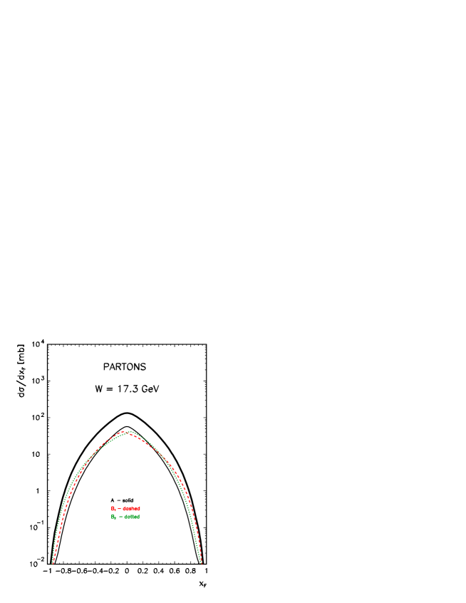
Figure 2: Distribution of virtually “produced” partons as a function of $x_{F}$ for W = 17.3 GeV and $b_{0}$ = 1 GeV^-1 of the Gaussian form factor. In this calculation 0.2 GeV $<p_{t}<$ 4 GeV. Contribution of diagram $A$ is shown by thin solid line, the contribution of diagram $B_{1}$ by dashed line and contribution of diagram $B_{2}$ by dotted line, and the sum of all processes by thick solid line.

In the familiar collinear approach the contributions of diagrams involving quarks and antiquarks are not negligible even at large energies. A nice, quantitative discussion of this issue can be found in [3]. In this section we shall make a similar analysis in our approach based on CCFM uPDF’s. In Fig.2 we display the contributions of partons (gluons, quarks, and antiquarks) for all diagrams of Fig.1 for the center-of-mass energy W = 17.3 GeV, i.e. energy of recent experiments of the NA49 collaboration at CERN as a function of jet (minijet) $x_{F}$. The parton rapidity is related to the parton $x_{F}$ as follows

$$y=\frac{1}{2}\log\left(\frac{\sqrt{m_{x}^{2}+x_{F}^{2}\frac{s}{4}+p_{t}^{2}}+x_{F}\frac{\sqrt{s}}{2}}{\sqrt{m_{x}^{2}+x_{F}^{2}\frac{s}{4}+p_{t}^{2}}-x_{F}\frac{\sqrt{s}}{2}}\;,\right)\;$$ (28)

where the parton mass here is the same as in Eq.(15). The corresponding cross section is obtained by integration over parton transverse momenta in the interval 0.2 GeV $<p_{t}<$ 4 GeV. The $gg\to g$ contribution, claimed to be the dominant contribution at RHIC [10], is somewhat smaller than the contribution of diagrams $B_{1}$ and $B_{2}$. The contribution of diagram $B_{1}$ (dashed line) dominates at negative Feynman-$x_{F}$, while the contribution of diagram $B_{2}$ (dotted line) at positive Feynman-$x_{F}$. By symmetry requirements $d\sigma^{B_{2}}/dx_{F}(x_{F})=d\sigma^{B_{1}}/dx_{F}(-x_{F})$.

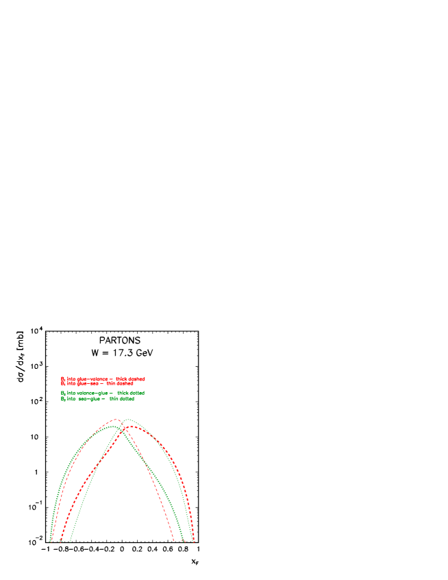
Figure 3: Decomposition of diagram $B_{1}$ cross section into glue-sea and glue-valence components and of diagram $B_{2}$ cross section into sea-glue and valence-glue components as a function of $x_{F}$.

In order to understand the intriguing asymmetry in $x_{F}$ of contributions of diagrams $B_{1}$ and $B_{2}$, in Fig.3 we present a further decomposition of the $B_{1}$ contribution into sea-glue, valence-glue subcontributions and correspondingly of the $B_{2}$ contribution into glue-sea, glue-valence subcontributions. This decomposition shows that the sea-glue and glue-sea contributions are of similar size as the valence-glue and glue-valence, respectively. It is interesting to note a different $x_{F}$-asymmetry of the contributions involving sea and valence quarks. This decomposition explains the shift of maxima of contributions corresponding to diagram $B_{1}$ and $B_{2}$ seen in Fig.2.

For completeness in Fig.4 we show transverse momentum distribution of “produced” gluons corresponding to diagram $A$ and of quarks and antiquarks corresponding to diagrams $B_{1}$ and $B_{2}$. In this calculation we have integrated over parton $x_{F}$ (or parton rapidity). For the two contributions one obtains a rather similar functional behaviour. It is worth noticing that in contrast to the standard collinear case in our approach the partonic cross section is fully integrable. This seems promissing in extending the region of applicability of the “perturbative” QCD towards smaller transverse momenta of hadrons.

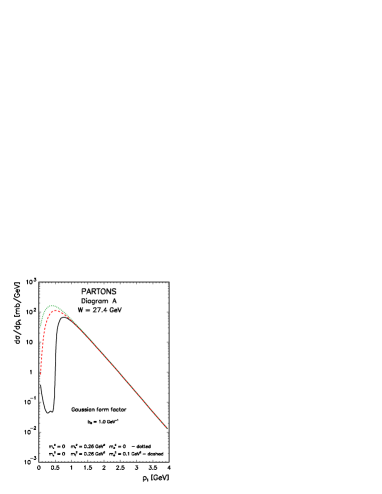
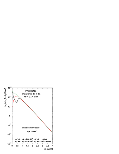
Figure 5: Transverse momentum distribution of partons from diagram $A$ (left panel), and $B_{1}+B_{2}$ (right panel) for W = 27.4 GeV and -1 $<x_{F}<$ 1. In this calculation $b_{0}$ = 1 GeV^-1. The solid line is the same as in the previous figure, i.e. freezing prescription for the factorization scale was used. For comparison the dotted line includes the shift prescription for the factorization scale. Finally the dashed line includes shift of factorization scale and modification of denominator as described in the text.

The rise of the cross section above $p_{t}\approx$ 0.5 GeV is due to a rapid increase of gluonic radiation above $p_{t}=\mu_{0}$, where $\mu_{0}^{2}$ is the minimal factorization scale for the GRV parton distributions. On the other hand, the rise of the cross section towards $p_{t}<\mu_{0}$ is an artifact of freezing factorization scale below $\mu_{0}^{2}$ in the conjuction of the singular behaviour of the denominator in the parton cross section formulae. To elucidate this issue somewhat better in Fig.5 we present also the results with the second prescription for the factorization scale with the minimal shift of the factorization scale (dotted line) and the result with an extra substitution of $\frac{1}{p_{t}^{2}}$ by $\frac{1}{p_{t}^{2}+m_{d}^{2}}$ (dashed line), where $m_{d}^{2}$ is a new nonperturbative parameter of our model specified in the figure. The second low-scale prescription lead to a smooth behavior of the partonic cross section at low transverse momenta. The consequences and the sensitivity to the extra prescription on the pion production at low transverse momenta of hadrons will be discussed in the next section.

5.2 Pion distributions

The passage from parton distributions to hadron distributions is the next step of our analysis. In the present approach we shall use the approach based on phenomenological fragmentation functions known from other processes. In the literature it is mostly $e^{+}e^{-}\to$ hadrons reactions which are used for extraction of phenomenological fragmentation functions.

There are a few sets of fragmentation functions in the literature. In the present calculation we shall use the fragmentation function of Kretzer [25]. There are two advantages of this particular set of fragmentation functions over other known from the literature. Firstly, the Kretzer fragmentation functions are available and reasonable even for very low scales $p_{t}\sim$ 1 GeV, or even less, i.e. in the region of our interest. Secondly, more attention in their construction was paid to the flavour structure than in any other approach in the literature. A good control of the flavour structure is essential when discussing and comparing contributions of diagram $A$, $B_{1}$ and $B_{2}$ to the pion momentum distributions.

In Fig.6 we compare our model invariant cross sections for $pp\to\pi^{+}$ (left panel) and $pp\to\pi^{-}$ (right panel) as a function of pion transverse momentum at W = 27.4 GeV for different values of the parameter $b_{0}$ of our Gaussian nonperturbative form factor. In principle, our result should not exceed experimental data especially in the perturbative regime of $p_{t}>$ 2 GeV where the perturbative $2\to 2$ parton subprocesses are crucial. This limits the value of the nonperturbative form factor to $b_{0}>$ 0.5 GeV^-1.

As can be seen from the figure the agreement of our model with experimental data is not perfect. There can be a few reasons for this fact. In order to understand the problem somewhat better let us concentrate on a small transverse momentum region $p_{t,h}<$ 2 GeV. As an example in Fig.7 we present our results for $b_{0}$ = 1 GeV^-1. We observe a deficit at $p_{t}>$ 0.5 GeV and a strong excess at $p_{t}<$ 0.3 GeV. It is particularly intriguing which effect stands behind the huge excess at very small transverse momenta. In addition, in Fig.7 we present contributions of different disjoint and complementary regions of variable $z$, as indicated in the figure. The figure shows that the rapid increase below $p_{t}\sim$ 0.3 GeV is caused exclusively by small $z<$ 0.2 i.e. must be traced back to the phenomenological fragmentation functions used. The Kretzer fragmentation functions as calculated from the publicly available computer code [26] are restricted to factorization scales larger than 1 GeV². Therefore in our calculation we were forced to freeze the fragmentation functions below $\mu_{D}=p_{t}<$ 1 GeV. The fragmentation functions at this small scale are shown by the solid line in Fig.8 for illustration. A clear rise of the fragmentation functions at small z can be observed, which in conjunction with the previous observation must be responsible for the excess of pions at very small $p_{t,h}$. The lower limit for the scale of about 1 GeV² is a recomendation based on analysis of the $e^{+}e^{-}$ data rather than a rigorous applicability limit. In fact, the initial evolution scale in [25] is $\mu_{0}^{2}$ = 0.26 GeV². Let us try to use the Kretzer fragmentation functions at this even lower scale. In Fig.8 we show (dashed line) the gluon and quark fragmentation functions. While for $g\to\pi$ fragmentation the small-z rise in “z D(z)” completely dissapears and a minimum at z = 0 is obtained (valence-like character), for the quark fragmentation only a saturation of “z D(z)” can be observed. In Fig.9 we show the result for pion production obtained with the fragmentation function at the lowest factorization scale $\mu_{0}^{2}$ = 0.26 GeV². Clearly the description of the data is now better. It is somewhat amusing that even the description above $p_{t,h}$ = 0.5 GeV is now much better. It becomes obvious that the choice of the factorization scale is very important in this context.

The description below $p_{t,h}$ = 0.2 GeV is still rather poor. This is partially caused by the behaviour of the quark fragmentation functions at small z (see Fig.8). Other effects are also possible. For example, we have used a simple one-parameter Gaussian form factor. In principle, such form factor may have more complicated functional dependence and can depend not only on the impact parameter, but also on energy and/or $x_{1}$ and $x_{2}$. Furthermore the whole formalism with z-dependent fragmentation functions must ultimately break at very low transverse momenta, in particular at small $x_{F}$ where resonance decays must be treated explicitly. Having this in view our final result seems promissing for further improvements in the future.

Inclusion of diagrams $B_{1}$ and $B_{2}$ in conjunction with the flavour dependent fragmentation functions lead to the $\pi^{+}-\pi^{-}$ asymmetry. In Fig.10 we show the asymmetry as the function of pion transverse momentum. The asymmetry is well described by our model, in contrast to individual distributions. This seems to suggest the right relative contributions of diagram $A$, $B_{1}$ and $B_{2}$. The asymmetry depends only weakly on the value of the parameter $b_{0}$ of the Gaussian nonperturbative form factor.

At SPS energies it is often customary to use $x_{F}$ rather than rapidity. The hadron Feynman variable $x_{F,h}$ is related to hadron pseudorapidity $\eta_{h}$ as

$$\eta_{h}=\frac{1}{2}\log\left(\frac{\sqrt{x_{F,h}^{2}\frac{s}{4}+p_{t,h}^{2}}+x_{F,h}\frac{\sqrt{s}}{2}}{\sqrt{x_{F,h}^{2}\frac{s}{4}+p_{t,h}^{2}}-x_{F,h}\frac{\sqrt{s}}{2}}\right)$$ (29)

and the jacobian of transformation expressed by $x_{F,h}$ and $p_{t,h}$ is

$$\frac{d\eta_{h}}{dx_{F,h}}=\frac{\frac{1}{2}\sqrt{s}}{\sqrt{x_{F,h}^{2}\frac{s}{4}+p_{t,h}^{2}}}\;.$$ (30)

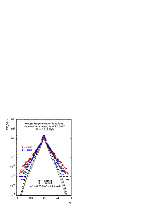
Figure 11: Our result against the UrQMD (red triangles) and HIJING (blue squares) models for SPS energy W = 17.3 GeV, for positive (dashed) and negative (dotted) pions. Thin lines correspond to Fig.7 and thick lines to Fig.9.

In Fig.11 we compare the $x_{F}$ distributions obtained in our approach for $b_{0}$ = 1 GeV² with those from some popular programs available on the market. The thin and thick (dashed and dotted) lines correspond to the different treatment of the scale in the fragmentation functions as described above (see also the figure caption). Clearly some mechanisms at large $x_{F}$ are missing in our approach. One of such mechanisms is the so-called pion stripping discussed e.g. in Ref.[30]. It was not our goal to include all of these effects and describe the experimental data. Our intention here was to identify the dominant mechanisms in the language of unintegrated parton distributions adequate at intermediate and low transverse momenta.

For completeness in Fig.12 we present a decomposition of the pion $x_{F}$ distribution into the components corresponding to diagrams shown in Fig.1. The purely gluonic contribution (diagram $A$) is comparable to the other two contributions at $x_{F}\approx$ 0, but at $|x_{F}|>$ 0.5 the contributions of diagram $B_{1}$ and $B_{2}$ are significantly larger. Similarly as for parton distributions the diagrams $B_{1}$ and $B_{2}$ contribute at somewhat larger $|x_{F}|$ than the diagram $A$. Some differences for $\pi^{+}$ and $\pi^{-}$ distributions are visible in the figure. The mechanisms underlying diagrams $B_{1}$ and $B_{2}$ are important contributors to understand the $\pi^{+}-\pi^{-}$ asymmetry at small and intermediate values of $x_{F}$. We think, however, that the dominant mechanism of $\pi^{+}$ and $\pi^{-}$ asymmetry in very forward ($x_{F}>$ 0.5) and very backward ($x_{F}<$ -0.5) hemispheres is due to the pion stripping mechanism (for a reference see e.g. [30]).

6 Conclusions

The approach based on unintegrated gluon distributions was applied recently to describe particle momentum distributions at RHIC for nucleus-nucleus [10] and proton-proton collisions [11]. We propose new mechanisms, neglected so far in the literature, which involve also quark/antiquark degrees of freedom and are based on (anti)quark-gluon and gluon-(anti)quark fusion processes followed by the subsequent fragmentation. These missing mechanisms have been estimated in the approach based on unintegrated parton (gluon, quark, antiquark) distributions originating from the solution of a set of coupled equations proposed recently by Kwieciński and coworkers. The formalism proposed recently by Kwieciński is very useful to obtain not only gluon unintegrated distributions but also their counterparts for quarks and antiquarks.

In the present paper we have concentrated on low energies $W\sim$ 20 GeV, relevant for SPS experiments. By freezing relevant scales for small parton transverse momenta we achieve a reasonable description of the data down to pion transverse momenta $\sim$ 0.5 GeV. The missing terms lead to an asymmetry in the production of the $\pi^{+}$ and $\pi^{-}$ mesons. While at lower energies of the order of 20 – 50 GeV such an asymmetry has been observed experimentally, it was not yet studied at RHIC. The BRAHMS collaboration at RHIC has a potential to study the asymmetries. Such asymmetries may be also useful to pin down the non-gluonic mechanisms as those encoded in diagrams $B_{1}$ and $B_{2}$.

The non-ideal agreement with the experimental data at low $p_{t}$ can be due to approximate treatment of nonperturbative effects embodied in the form factors, as well as in the treatment of hadronization effects with the help of scale-dependent one-parameter fragmentation functions. Both these effects require further detailed studies which go beyond the scope of the present paper.

Acknowledgements We are indebted to Peter Levai for an interesting discussion about collinear approach and Stefan Kretzer for a discussion about parton fragmentation functions. We are also indebted to Ewa Kozik and Piotr Pawłowski for performing the calculation with the UrQMD and HIJING code, respectively. This work was partially supported by the Polish KBN grant no. 1 P03B 028 28.

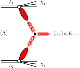
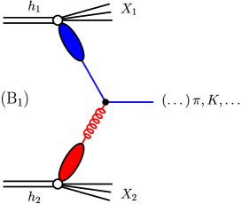
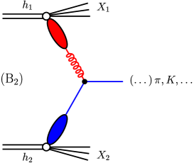
Figure 1: Leading-order diagrams for inclusive parton production

Figure 4: Transverse momentum distribution of partons from diagram $A$ (left panel), and $B_{1}+B_{2}$ (right panel) for W = 27.4 GeV and different values of the Gaussian form factor. The cross sections presented were obtained through integration over -1 $<x_{F}<$ 1.

Figure 6: Invariant cross section as a function of transverse momentum of $\pi^{+}$ (left panel) and $\pi^{-}$ (right panel) for $\eta$ = 0, W = 27.4 GeV and different values of parameter in the Gaussian form factor. Experimental data for W = 23, 31 GeV from [27] and for W = 27.4 GeV [28] are shown for comparison.

Figure 7: Invariant cross section as a function of transverse momentum of $\pi^{+}$ (left panel) and $\pi^{-}$ (right panel) for $\eta$ = 0, W = 27.4 GeV. In this calculation $b_{0}$ = 1 GeV^-1.

Figure 8: The basic Kretzer fragmentation functions at low factorization scales.

Figure 9: Invariant cross section as a function of transverse momentum of $\pi^{+}$ (left panel) and $\pi^{-}$ (right panel) for $\eta$ = 0, W = 27.4 GeV obtained with the Kretzer fragmentation functions at $\mu_{0}^{2}$ = 0.26 GeV². In this calculation $b_{0}$ = 1 GeV^-1.

Figure 10: Ratio of cross sections from Fig.6 as a function of pion transverse momentum for W = 27.4 GeV.

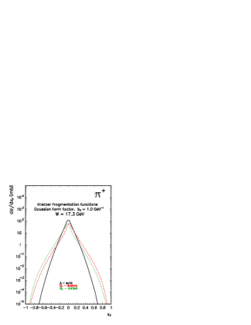
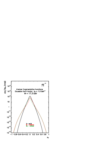
Figure 12: Contribution of diagrams $A$ (thin solid), $B_{1}$ (dashed) and $B_{2}$ (dotted) to charged-pion $x_{F}$ distributions for W = 17.3 GeV. In this calculation $b_{0}$ = 1.0 GeV^-1 and 0.2 GeV $<p_{t,h}<$ 2 GeV.

References

- [1] J.F. Owens, Rev. Mod. Phys. 59 (1987) 465.
- [2] R. D. Field, Application of Perturbative QCD (Addison-Wesley, Reading, MA, 1995).
- [3] K.J. Eskola and K. Kajantie, Z. Phys. C75 (1997) 515.
- [4] K.J. Eskola and H. Honkanen, Nucl. Phys. A713 (2003) 167.
- [5] G.G. Barnafoldi, G. Fai, P. Levai, G. Papp, Y. Zhang, J. Phys. G27 (2001) 1767.
- [6] X.-N. Wang, Phys. Rev. C61 (2000) 064910.
- [7] Y. Zhang, G. Fai, G. Papp, G.G. Barnafoldi and P. Levai, Phys. Rev. C65 (2002) 034903.
- [8] G. Papp, G.G. Barnafoldi, P. Levai and G. Fai, hep-ph/0212249.
- [9] Ch.-Y. Wong and H. Wang, Phys. Rev. C58 (1998) 376.
- [10] D. Kharzeev and E. Levin, Phys. Lett. B523 (2001) 79.
- [11] A. Szczurek, Acta Phys. Polon. B34 (2003) 3191.
- [12] A. Szczurek, Acta Phys. Polon. B35 (2004) 161.
-
[13]
Proceedings of the Quark Matter 2002 conference, July 2002,
Nantes, France; Nucl. Phys. A715 (2003).
Proceedings of the Quark Matter 2004 conference, January 2004, Oakland, USA; J. Phys. G30 (2004). - [14] B.B. Back et al. (PHOBOS collaboration), Phys. Rev. Lett. 87 (2001) 102303-1.
- [15] I.G. Bearden et al. (BRAHMS collaboration), Phys. Rev. Lett. 87 (2001) 112305.
- [16] L.V. Gribov, E.M. Levin and M. G. Ryskin, Phys. Lett. B100 (1981) 173.
- [17] M.A. Kimber and A.D. Martin and M.G. Ryskin, Phys. Rev. D63 (2001) 114027-1.
- [18] J. Kwieciński, Acta Phys. Polon. B33 (2002) 1809.
- [19] A. Gawron and J. Kwieciński, Acta Phys. Polon. B34 (2003) 133.
- [20] A. Gawron, J. Kwieciński and W. Broniowski, Phys. Rev. D68 (2003) 054001.
- [21] J. Kwieciński and A. Szczurek, Nucl. Phys. B680 (2004) 164.
- [22] M. Łuszczak and A. Szczurek, Phys. Lett. B594 (2004) 291.
- [23] D.V. Shirkov and I.L. Solovtsov, Phys. Rev. Lett. 79 (1997) 1209.
- [24] J. Binnewies, B.A. Kniehl, G. Kramer, Phys. Rev. D52 (1995) 4947.
- [25] S. Kretzer, Phys. Rev. D62 (2000) 054001.
- [26] S. Kretzer, private communication.
- [27] B. Alper et al. (British-Scandinavian collaboration), Nucl. Phys. B100 (1975) 237.
- [28] D. Antreasyan et al., Phys. Rev. D19 (1979) 764.
- [29] M. Glück, E. Reya and A. Vogt, Eur. Phys. J. C5 (1998) 461.
- [30] N.N. Nikolaev, W. Schäfer, A. Szczurek and J. Speth, Phys. Rev. D60 (1999) 014004.